Self-sustained magnetoelectric oscillations in magnetic resonant tunneling structures

Abstract

The dynamic interplay of transport, electrostatic, and magnetic effects in the resonant tunneling through ferromagnetic quantum wells is theoretically investigated. It is shown that the carrier-mediated magnetic order in the ferromagnetic region not only induces, but also takes part in intrinsic, robust, and sustainable high-frequency current oscillations over a large window of nominally steady bias voltages. This phenomenon could spawn a new class of quantum electronic devices based on ferromagnetic semiconductors.

Ferromagnetism of diluted magnetic semiconductors (DMSs), such as GaMnAs Ohno (1998), depends strongly on the carrier density Dietl et al. (1997); Dietl (2007); Jungwirth et al. (2006); Lee et al. (2002); Jungwirth et al. (1999). The possibility to tailor space charges in semiconductors by bias or gate fields naturally suggests similar tailoring of magnetic properties of DMSs. While early experiments have indeed succeeded in generating ferromagnetism in DMSs electrically or optically Ohno et al. (2000); Boukari et al. (2002), ramifications of the strong carrier-mediated ferromagnetism in the transport through DMS heterostructures are largely unexplored.

In resonant tunneling through a quantum well not only the tunneling current, but also the carrier density in the well are sensitive to the alignment of the electronic spectra in the leads and in the well. If the quantum well is a paramagnetic DMS, the resulting transport is influenced by the spin splitting of the carrier bands in the well, as observed experimentally Slobodskyy et al. (2003). The magnetic resonant diodes are prominent spintronic devices Fabian et al. (2007); Žutić et al. (2004), proposed for spin valves and spin filtering Petukhov et al. (2002); Ertler and Fabian (2006a), or for digital magnetoresistance Ertler and Fabian (2006b); Ertler and Fabian (2007).

If the quantum well is made of a ferromagnetic DMS Oiwa et al. (2004); Ohya et al. (2007), resonant tunneling conditions should influence magnetic ordering as well. It has already been predicted that the critical temperature $T_{c}$ of the well can be strongly modified electrically Ganguly et al. (2005); Fernández-Rossier and Sham (2002); Lee et al. (2000, 2002). Here we show that the magnetic ordering affects back the tunneling current, in a peculiar feedback process, leading to interesting dynamic transport phenomena.

Conventional nonmagnetic RTDs can exhibit subtle intrinsic bistability and terahertz current oscillations Ricco and Azbel (1984); Jona-Lasinio et al. (1992); Orellana et al. (1997); Jensen and Buot (1991); Zhao et al. (2003) resulting from the nonlinear feedback of the stored charge in the quantum well. Interesting phenomena occur also in multiple quantum wells and superlattices, in which electric field domains form whose dynamics leads to current oscillations in the kHz-GHz range Bonilla and Grahn (2005). This effect has been exploited for spin-dependent transport by incorporating paramagnetic quantum wells Sánchez et al. (2001); Béjar et al. (2003).

In this article we introduce a realistic model of a self-consistently coupled transport, charge, and magnetic dynamics and apply it to generic asymmetric resonant diodes with a ferromagnetic quantum well to predict self-sustained, stable high-frequency oscillations of the electric current and quantum well magnetization. We formulate a qualitative explanation for the appearance of these magnetoelectric oscillations. In essence, ferromagnetic quantum wells exhibit strong nonlinear feedback to the electric transport since the ferromagnetic order, which gives rise to the exchange splitting of the quantum well subbands, is itself mediated by the itinerant carriers. This together with the Coulomb interaction which effectively modifies the single electron electrostatic potential in the well, leads to a strong coupling of the transport, electric, as well as magnetic properties of ferromagnetic resonant tunneling structures.

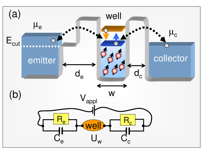
Figure 1: (Color online) (a) Schematic scheme of the band profile of the magnetic double barrier structure. The exchange interaction of the magnetic ions is mediated by the carriers tunneling in and out of the well. Here, the cut off of the emitter tunneling rate is realized by a cascaded left barrier. (b) Equivalent circuit model of the resonant tunneling structure introducing the emitter and collector capacitances $C_{e},C_{c}$ and resistances $R_{e},R_{c}$, respectively.

Our model resonant tunneling structure with a ferromagnetic well made of a DMS-material, e.g., GaMnAs, is sketched in Fig. 1(a). To exhibit magnetoelectric oscillations the structure needs a built-in energy cut-off, $E_{\mathrm{cut}}$, of the emitter tunneling rate. Such an energy cut-off might be realized by a cascaded left barrier, as shown in Fig. 1(a), by which the tunneling for carriers with energies smaller than $E_{\mathrm{cut}}$ is exponentially suppressed, due to the increased barrier width. Other possibilities to realize the cutoff are discussed below.

As we aim to understand the most robust features of the ferromagnetic resonant tunnel structures, we present a minimal theoretical model which captures the essential physics. The longitudinal transport through the system can be described in terms of sequential tunneling, as the high densities of magnetic impurities residing in the ferromagnetic well will likely cause decoherence of the propagating carries. Based on the transfer Hamiltonian formalism a master equation for the semiclassical particle distribution in the well can be derived, as described elsewhere Fabian et al. (2007); Averin et al. (1991). We assume that there is only a single resonant well level $E_{0}$ in the energy range of interest, allowing us to write the rate equations for the spin-resolved, time dependent quantum well particle densities $n_{\sigma}(t),(\sigma=\uparrow,\downarrow=\pm 1/2)$ as,

$$\frac{\mathrm{d}n_{\sigma}}{\mathrm{d}t} = \Gamma_{e}(E_{\sigma})\>n_{e,\sigma}+\Gamma_{c}(E_{\sigma})\>n_{c,\sigma}-\Gamma(E_{\sigma})\>n_{\sigma}$$ (1)

$$-\frac{n_{\sigma}-n_{0,\sigma}}{\tau_{s}}.$$

Here, $\Gamma_{\{e,c\}}$ denotes the energy-dependent tunneling rate from the emitter (e) and the collector (c), $\Gamma=\Gamma_{e}+\Gamma_{c}$ denotes the total tunneling rate, $\tau_{s}$ stands for the spin relaxation time in the well, $n_{0,\sigma}$ denotes the quasiequilibrium particle spin density, and $n_{\sigma,\{e,c\}}$ are the densities of particles in the emitter and collector reservoir, respectively, having the resonant longitudinal energy $E_{\sigma}$. The spin-split resonant energies are

$$E_{\sigma}=E_{0}+U_{w}-\sigma\Delta,$$ (2)

with $U_{w}$ being the electrostatic well potential and $\Delta$ denoting the subband exchange splitting. The total energy of the particles $E_{\mathrm{tot}}$ is then given by the sum of the longitudinal energy $E_{\sigma}$ and the in-plane kinetic energy: $E_{\mathrm{tot}}=E_{\sigma}+T_{\mathrm{in}}$. The physical meaning of the right side of Eq. (1) is as follows: the first two terms are the gain terms, describing tunneling from the emitter and the collector into the well; the third term describes all loss processes due to the tunneling out of the well, and the last term models the spin relaxation in the well. Considering the Fermi-Dirac distributions in the emitter and the collector, the particle densities $n_{i,\sigma}$ are,

$$n_{i,\sigma}=D_{0}k_{B}T\ln\left\{1+\exp\left[(\mu_{i}-E_{\sigma})/k_{B}T\right]\right\}\quad i=e,c,$$ (3)

with $k_{B}$ denoting Boltzmanns’ constant; $T$ is the lead temperature, $\mu_{i}$ are the emitter and collector chemical potentials with $\mu_{c}=\mu_{e}-eV_{\mathrm{appl}}$ where $V_{\mathrm{appl}}$ is the applied bias, and $D_{0}=m/2\pi\hbar^{2}$ is the two-dimensional density of states per spin for carriers with the effective mass $m$. The tunneling rates are essentially given by the overlap of the lead and well wave functions according to Bardeen’s formula Bardeen (1961). For high barriers the rate becomes proportional to the longitudinal momentum $p_{z}$ of the particles Averin et al. (1991), i.e., $\Gamma_{e,c}\propto(E_{z})^{1/2}$ with $E_{z}$ denoting the longitudinal energy.

In the framework of a mean field model for the carrier mediated ferromagnetism in heterostructure systems Dietl et al. (1997); Jungwirth et al. (1999); Lee et al. (2002); Fabian et al. (2007) the steady state exchange splitting of the well subbands is determined by

$$\Delta_{0} = J_{\mathrm{pd}}\int\mathrm{d}z\>n_{\mathrm{imp}}(z)\left|\psi_{0}(z)\right|^{2}$$ (4)

$$\times SB_{S}\left[\frac{SJ_{\mathrm{pd}}s(n_{\downarrow}-n_{\uparrow})\left|\psi_{0}(z)\right|^{2}}{k_{B}T}\right].$$

Here, $J_{\mathrm{pd}}$ denotes the coupling strength between the impurity spin and the carrier spin density (in case of GaMnAs p-like holes couple to the d-like impurity electrons), $z$ is the longitudinal (growth) direction of the structure, $n_{\mathrm{imp}}(z)$ is the impurity density profile, $\psi_{0}(z)$ labels the well wave function, $B_{S}$ denotes the Brillouin function of order $S$, and $S$ and $s=1/2$ are the impurity and particle spin, respectively. (In the case of Mn impurities S = 5/2.) The expression shows that the well spin-splitting depends basically on the particle spin polarization $\xi=n_{\downarrow}-n_{\uparrow}$ in the well and the overlap between the wave function and the impurity band profile. For simplicity, we consider here a homogenous impurity distribution in the well, which makes $\xi$ the determining factor for $\Delta_{0}$.

After a sudden change of the well spin polarization the magnetic impurities need some time to respond until the corresponding mean field value $\Delta_{0}$ is established. In the case of GaMnAs, experimental studies of the magnetization dynamics revealed typical response times of about 100 ps Wang et al. (2007). We model the magnetization evolution within the relaxation time approximation, $\mathrm{d}\Delta/\mathrm{d}t=-(\Delta-\Delta_{0})/\tau_{\Delta}$, with $\tau_{\Delta}$ denoting the well spin-splitting relaxation time.

Finally, to take into account the nonlinear feedback of the Coulomb interaction of the well charges, we introduce emitter-well and collector-well capacitances, $C=C_{e}+C_{c}$ according to the equivalent circuit model of a resonant tunneling diode, as shown in Fig. 1(b). The capacitances $C_{e}$ and $C_{c}$ are determined by the geometrical dimensions of the barriers and the well Averin et al. (1991). The electrostatic well potential can then be written as

$$U_{w}=\frac{1}{C}\left[e^{2}(n-n_{\mathrm{back}})-C_{c}eV_{\mathrm{appl}}\right]$$ (5)

with $e$ denoting the elementary charge, $n_{\mathrm{back}}$ is the positive background charge (from magnetic donors) in the well. All the equations are nonlinearly coupled via Eq. (2) for the resonant well levels $E_{\sigma}$, making a numerical solution indispensable.

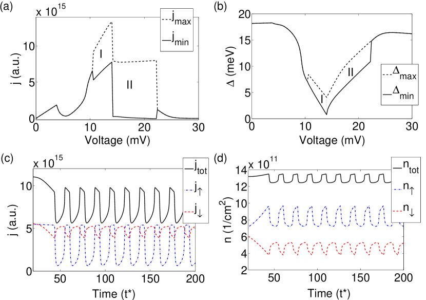
Figure 2: (Color online) (a) Current-voltage (IV)-characteristic of the investigated structure at the energy cut-off $E_{\mathrm{cut}}=85$ meV. In the unsteady region between 11 to 22 mV the current does not reach a steady state value; instead intrinsic current oscillations appear, in which both the maximum and minimum values of the oscillations are indicated by the dashed and solid lines, respectively. Two different dynamic modes I and II can be identified. (b) Well splitting $\Delta$ versus applied voltage. In the unsteady region the maximum (dashed) and minimum (solid) values of the magnetization oscillations are plotted. (c) and (d) Transients of the spin-resolved current $j$ and the well particle density $n$ at the applied voltage $V=12$ mV and $E_{\mathrm{cut}}=85$ meV. The time is measured in units of $t^{*}$ (typically some picoseconds) as explained in the text.

In the numerical simulations we use generic parameters assuming a GaMnAs well: $m=0.5\>m_{0}$, $\varepsilon_{r}=12.9$, $d_{e}=50$ Å, $d_{c}=20$ Å, $w=10$ Å, $\mu_{e}=100$ meV, $n_{\mathrm{imp}}=1.5\times 10^{20}$cm^-3, $J_{\mathrm{pd}}=0.06$ eV nm³, $\tau_{s}=1\>t^{*}$, $\tau_{\Delta}=10\>t^{*}$, where $d_{e},d_{c}$ and $w$ are the emitter barrier, collector barrier and quantum well widths, $m_{0}$ denotes the free electron mass, and $\varepsilon_{r}$ is the relative permittivity of the well. The characteristic time scale $t^{*}$ is the inverse emitter tunneling rate at the emitters’ Fermi energy, $[t^{*}=1/\Gamma_{e}(\mu_{e})]$, being of the order of picoseconds. For the well background charge we consider that in GaMnAs the actual carrier density is only about 10% of the nominal Mn doping density Das Sarma et al. (2003): $n_{\mathrm{back}}=0.1\>n_{\mathrm{imp}}$. Our calculations are performed at $T=4.2$ K, which is well below the critical temperature of our specific well $T_{c}\approx 10$ K, where we estimated $T_{c}$ by using the mean-field result given in Ref. Lee et al. (2000).

Figure 2(a) shows the current-voltage (IV) characteristic of the structure. Up to about V = 11 mV the typical peaked IV-curve of a resonant tunneling diode is obtained. However, in the voltage range of 11 to 22 meV, which we will call hereafter the “unsteady” region, the current does not settle down to a steady state value; instead stable high-frequency oscillations occur, as shown in Fig. 2(c) for the applied voltage of $V=12$ mV. The current is always evaluated at the collector side: $j_{c,\sigma}=\Gamma_{c}(E_{\sigma})(n_{\sigma}-n_{c,\sigma})$. Along with the current, oscillations of the well magnetization as well as of the spin densities appear, as shown in Fig 2(b) and (d). Those magneto-electric oscillations are the main results of this paper.

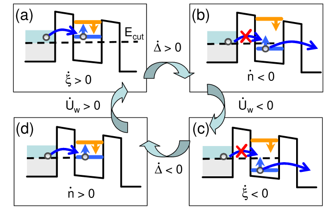
Figure 3: (Color online) Explanation for the occurrence of self-sustained oscillations in the case of mode I. For mode II the arguments are completely analogous but there the spin down level is crossing the cut-off energy $E_{\mathrm{cut}}$. (a) According to the in-tunneling spin-up carriers the spin polarization $\xi$ is increased, giving rise to an increasing well splitting $\Delta$. (b) When the spin up level falls below the cutoff energy the total particle number decreases and, hence, also the electrostatic potential $U_{w}$ does. (c) This pushes the spin-up level even deeper into the cut-off region leading to a fast decrease of the spin polarization and consequently of the well splitting, which brings the spin up level back to the emitter’s supply region (d), restarting the whole cycle.

The IV-curve in the unsteady region suggests the existence of two qualitatively different dynamic modes. Indeed, comparing the transients in these two voltage regions reveals that in region I the spin up level is recurringly crossing the emitter energy cut off $E_{\mathrm{cut}}$, whereas in region II this is done by the spin down level, as schematically illustrated in Fig. 3. This insight offers the following explanation for the the occurrence of self-sustained oscillations. Take mode I; the arguments for mode II are similar. The dropping of the spin up level below the cut-off energy (due to the increasing exchange splitting) as two implications: (i) the supply of the emitter spin up electrons sharply decreases. Hence, the total well particle density $n=n_{\uparrow}+n_{\downarrow}$ decreases because the spin up electrons residing in the well are tunneling out to the collector. A decreased particle density leads to a decreased electrostatic potential according to Eq. (5), which effectively drives the spin up level even deeper into the cut-off region. (ii) Since the spin up electrons are the majority spins in the well, a decrease of $n_{\uparrow}$ implies a decreasing spin polarization $\xi$ in the well. This causes, via Eq. (4), a rapid decrease of the subband exchange splitting, bringing the spin up level back to the emitter supply region. The spin up electrons can then tunnel again into the well and the whole process starts from the beginning, producing the calculated cycles.

The occurrence of these oscillations needs the concurrent interplay of both the electric and magnetic feedbacks: the electrostatic feedback acts like an “inertia” for the oscillations, allowing the spin level to get deeper into the cut-off region, whereas the magnetic feedback is needed to bring the level back into the emitter’s supply region. From the above discussions it also follows that a steep descent in the tunneling rate at the cut-off energy is necessary. This is confirmed in our simulations, where we assumed an exponential decay of $\Gamma_{E}$ for $E_{z}<E_{\mathrm{cut}}$. Actually, this is also the reason why no oscillations are occurring at the emitter’s conduction band edge $(E_{z}=0)$, which is an otherwise natural emitter’s cut-off, because near the band edge the tunneling rate is already almost vanishing according to $\Gamma_{E}\propto(E_{z})^{1/2}$.

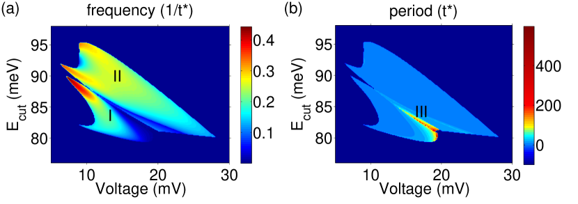
Figure 4: (Color online) Contour plots of the frequency (a) and the period (b) of the intrinsic oscillations as a function of the applied voltage and the cut-off energy $E_{\mathrm{cut}}$. The two islands of high-frequency oscillations correspond to the dynamic modes I and II. They are separated by a crossover region III of high-period oscillations, which becomes most evident in period contour plot (b).

The typical timescale for the oscillations is made up by two contributions: (i) the evolution of the well splitting $\Delta$ in the emitter’s supply region, i.e., the time needed for the well splitting $\Delta$ to become large enough that one of the spin levels crosses the cut off energy, and (ii) the dynamics of $\Delta$ in the cut-off region. The timescale of contribution (i) can be estimated to be proportional to $\tau_{\Delta}(r-1)$, where $r$ is the ratio of the well splitting when the cut-off energy is reached to the initial splitting at the beginning of the cycle, whereas the dynamics of contribution (ii) is mostly governed by a fast rearrangement of the spin densities in the well, which happens on the order of the tunneling time $t^{*}$. This is in line with the numerical result that the oscillation frequency increases with decreasing $\tau_{\Delta}$. In contrast, a decreasing spin relaxation time, which diminishes more and more effectively the spin polarization in the well and, hence, the well splitting, gives rise to a decrease of the frequency.

The fastest magnetoelectric oscillations in our simulations for the generic parameters used exhibit periods of about $2.5\times t^{*}\approx 5$ ps. Important, the oscillation frequency can be modified by varying the applied voltage, as can be seen in Fig. 4, which displays contour plots of the frequency and the period versus the applied voltage and the cut-off energy. Two “islands” can be distinguished, corresponding to the two regions of the dynamic modes I and II, respectively (see Fig. 2). Mode II appears at higher voltages, where the collector chemical potential is already below the cut-off energy. In this case the decrease of the well particle density is much stronger when the spin up level crosses the cut-off energy, as illustrated in Fig. 3(b), since none of the out-tunneling electrons are “Pauli-blocked” by the collector electrons. This gives rise to a much stronger decrease of the electrostatic potential as compared to mode I, pushing both the spin up and down levels below the cut-off energy. In the following oscillations this makes the spin down level recurringly crossing the cut-off energy instead of the spin up level as is the case for mode I.

Both modes are separated by a crossover region III, in which the oscillations have much longer periods than on the “islands”, as can be seen in Fig. 4(b). The reason for these low-frequency oscillations is that the initial spin polarization and, hence, the well splitting at the beginning of each cycle is small, yielding a large ratio $r$. Therefore, in region III it can take 10-100 times longer that the well splitting reaches the cut-off energy as for modes I or II. The possibility of controlling the frequency of the magnetoelectric oscillations by electrical means is especially interesting from the applications point of view.

For the experimental observation of the self-sustained oscillations the emitter needs to emit electrons in a sharply defined energy window. In the model above we propose an asymmetric barrier, as in Fig. 1(a). Another practical way would be using an auxiliary resonant tunneling structure in the emitter itself, providing a spectral filter allowing only resonant electrons to pass through. Yet another possibility would be employing a hot electron emitter, say using a Schottky barrier.

We have shown that the charge and magnetization dynamics in ferromagnetic tunneling heterostructures are influenced by the highly nonlinear feedback of both Coulomb and magnetic couplings on the tunneling transport. The feedback results in high-frequency self-sustained intrinsic oscillations suggesting applications of ferromagnetic QWs in tunable high-power current oscillators.

This work has been supported by the Deutsche Forschungsgemeinschaft SFB 689.

References

- Ohno (1998) H. Ohno, Science 281, 951 (1998).
- Dietl et al. (1997) T. Dietl, A. Haury, and Y. M. d’Aubigné, Phys. Rev. B 55, R3347 (1997).
- Dietl (2007) T. Dietl, in Modern Aspects of Spin Physics, edited by W. Pötz, J. Fabian, and U. Hohenester (Springer, Berlin, 2007), pp. 1–46.
- Jungwirth et al. (2006) T. Jungwirth, J. Sinova, J. Mašek, J. Kučera, and A. H. MacDonald, Rev. Mod. Phys. 78, 809 (2006).
- Jungwirth et al. (1999) T. Jungwirth, W. A. Atkinson, B. H. Lee, and A. H. MacDonald, Phys. Rev. B 59, 9819 (1999).
- Lee et al. (2002) B. Lee, T. Jungwirth, and A. H. MacDonald, Semi. Sci. Techn. 17, 393 (2002).
- Ohno et al. (2000) H. Ohno, D. Chiba, F. Matsukura, T. O. E. Abe, T. Dietl, Y. Ohno, and K. Ohtani, Nature 408, 944 (2000).
- Boukari et al. (2002) H. Boukari, P. Kossacki, M. Bertolini, D. Ferrand, J. Cibert, S. Tatarenko, A. Wasiela, J. A. Gaj, and T. Dietl, Phys. Rev. Lett. 88, 207204 (2002).
- Slobodskyy et al. (2003) A. Slobodskyy, C. Gould, T. Slobodskyy, C. R. Becker, G. Schmidt, and L. W. Molenkamp, Phys. Rev. Lett. 90, 246601 (2003).
- Fabian et al. (2007) J. Fabian, A. Matos-Abiague, C. Ertler, P. Stano, and Žutić, Acta Physica Slovaca 57, 565 (2007).
- Žutić et al. (2004) I. Žutić, J. Fabian, and S. Das Sarma, Rev. Mod. Phys. 76, 323 (2004).
- Ertler and Fabian (2006a) C. Ertler and J. Fabian, Appl. Phys. Lett. 89, 242101 (2006a).
- Petukhov et al. (2002) A. G. Petukhov, A. N. Chantis, and D. O. Demchenko, Phys. Rev. Lett. 89, 107205 (2002).
- Ertler and Fabian (2006b) C. Ertler and J. Fabian, Appl. Phys. Lett. 89, 193507 (2006b).
- Ertler and Fabian (2007) C. Ertler and J. Fabian, Phys. Rev. B 75, 195323 (2007).
- Oiwa et al. (2004) A. Oiwa, R. Moriya, Y. Kashimura, and H. Munekata, J. Magn. Magn. Mater. 272-276, 2016 (2004).
- Ohya et al. (2007) S. Ohya, P. N. Hai, Y. Mizuno, and M. Tanaka, Phys. Rev. B 75, 155328 (2007).
- Ganguly et al. (2005) S. Ganguly, L. Register, S. Banerjee, and A. H. MacDonald, Phys. Rev. B 71, 245306 (2005).
- Fernández-Rossier and Sham (2002) J. Fernández-Rossier and L. J. Sham, Phys. Rev. B 66, 73312 (2002).
- Lee et al. (2000) B. Lee, T. Jungwirth, and A. H. MacDonald, Phys. Rev. B 61, 15606 (2000).
- Ricco and Azbel (1984) B. Ricco and M. Y. Azbel, Phys. Rev. B 29, 1970 (1984).
- Jona-Lasinio et al. (1992) G. Jona-Lasinio, C. Presilla, and F. Capasso, Phys. Rev. Lett. 68, 2269 (1992).
- Orellana et al. (1997) P. Orellana, E. Anda, and F.Claro, Phys. Rev. Lett 79, 1118 (1997).
- Jensen and Buot (1991) K. L. Jensen and F. A. Buot, Phys. Rev. Lett. 66, 1078 (1991).
- Zhao et al. (2003) P. Zhao, D. L. Woolard, and H. L. Cui, Phys. Rev. B 67, 85312 (2003).
- Bonilla and Grahn (2005) L. L. Bonilla and H. T. Grahn, Rep. Prog. Phys. 68, 577 (2005).
- Sánchez et al. (2001) D. Sánchez, A. H. MacDonald, and G. Platero, Phys. Rev. B 65, 35301 (2001).
- Béjar et al. (2003) M. Béjar, D. Sánchez, G. Platero, and A. H. MacDonald, Phys. Rev. B 67, 45324 (2003).
- Averin et al. (1991) D. V. Averin, A. N. Korotkov, and K. K. Likharev, Phys. Rev. B 44, 6199 (1991).
- Bardeen (1961) J. Bardeen, Phys. Rev. Lett. 6, 57 (1961).
- Wang et al. (2007) J. Wang, I. Cotoros, K. M. Dani, X. Liu, J. K. Furdyna, and D. S. Chemla, Phys. Rev. Lett. 98, 217401 (2007).
- Das Sarma et al. (2003) S. Das Sarma, E. H. Hwang, and A. Kaminski, Phys. Rev. B 67, 155201 (2003).