Transverse momentum broadening of heavy quark and gluon energy loss in Sakai-Sugimoto model

Abstract

In this paper, we calculate the transverse momentum diffusion coefficient $\kappa_{T}$ of heavy quark and gluon penetration length in the deconfinement phase of Sakai-Sugimoto model, which is known as a holographic dual of large $\emph{N}_{c}$ QCD. We find that for the heavy quark moving through the thermal plasma with a constant velocity $v<1$, the transverse momentum diffusion coefficient $\kappa_{T}\propto\lambda\gamma^{\frac{1}{3}}\emph{T}^{4}/\emph{T}_{d}$, and the gluon penetration length $\triangle x\propto\hat{\emph{E}}^{\frac{2}{5}}$. These results are different from those calculated in $\mathcal{N}=4$ super-Yang-Mills theory, which are $\kappa_{T}\propto\lambda\gamma^{\frac{1}{2}}\emph{T}^{3}$ and $\triangle x\propto\hat{\emph{E}}^{\frac{1}{3}}$, respectively. In the high energy limit, the difference between the two pairs of results should be evident, so we hope that the future LHC experiments can tell us which model is more closely related to the realistic strongly coupled QCD at finite temperature.

USTC-ICTS-08-05

Transverse momentum broadening of heavy quark and gluon energy loss in Sakai-Sugimoto model

Yi Pang^2,1

¹ Interdisciplinary Center of Theoretical Studies, USTC,
Hefei, Anhui 230026, P.R.China
² Institute of Theoretical Physics, CAS, Beijing 100080, P.R.China

yipang@itp.ac.cn

1 Motivation

The experimental relativistic heavy ion collisions have produced much evidence signalling that Quark Gluon Plasma (QGP) has been formed at the Relativistic Heavy Ion Collision (RHIC) [1, 2]. One piece of strong evidence is that the production of the high-$p_{T}$ particles is suppressed [3, 4]. To explain this phenomenon within the framework of QCD is difficult, because recently, researchers have found that QGP is a strongly coupled fluid. In the framework of AdS/CFT [5], one can solve problems in strongly coupled gauge theories by considering the corresponding problems in dual weak coupled gravity theories. So, many people try to solve these problems in QGP, by transferring them into a gauge theory which has a gravity dual and can mimic QCD to some extent. Along this way, H. Liu, K. Rajagopal and U. Wiedemann define the jet quenching parameter $\hat{q}$, via a light-like Wilson loop [6]. ${\hat{q}}$ is the transverse momentum squared transferred from medium to either the initial parton or the radiated gluon, it is related to the average medium-induced parton energy loss by BDMPS formalism [24]. Meanwhile, J. Casalderrey-Solana, D. Teaney and S. Gubser prefer to use the transverse momentum coefficient $\kappa_{T}$ [8, 9, 10]. Although the two groups adopt different parameters, the calculations are both carried out in the same background, which is the $AdS_{5}$-Schwarzschild space-time. Subsequent work [12, 13, 14] includes computing ${\hat{q}}$ in backgrounds with non-zero chemical potential. Above all, the background metrics they use usually involve an asymptotically $AdS_{5}$ component, since the gravity theory in $AdS_{5}$ is dual to the $\mathcal{N}=4$ SYM, their results actually apply to $\mathcal{N}=4$ SYM. However $\mathcal{N}=4$ SYM is not the same as QCD, so it is problematic whether or not their results really capture some features of QCD, if it does, then these features should also appear in other models approximating QCD and having gauge/string duality, since all these models belong to one framework.

Fortunately, in paper [15], Sakai and Sugimoto provide us such an new model, which we call S-S model in this paper. This model is a holographic dual of four-dimensional, large $\emph{N}_{c}$ QCD in the low energy regime. In the high energy regime, the gauge theory in S-S model shows some differences from QCD, such as K-K modes. A lot of papers [16] have been done on this model, in which they recover some features similar to realistic QCD, such as confinement-deconfinement phase transition and chiral symmetry breaking-restoration phase transition. The calculations about screening length and jet quenching parameter $\hat{q}$ in this model [19, 18] have been carried out. But the transverse momentum diffusion coefficient $\kappa_{T}$ has not been obtained. To give a complete comparison between above two models, we calculate $\kappa_{T}$ in S-S model. During the preparation of this paper, S. Gubser et al [11] put forward a new approach to estimate the jet quenching parameter $\hat{q}$ by considering the gluon energy loss in the thermal plasma of strongly coupled $\mathcal{N}=4$ super-Yang-Mills theory. Using this new method, we estimate $\hat{q}$ in S-S model. If we did not try this new way in S-S model, the comparison between the two models is still incomplete.

This paper is organized as follows. In Section 2 we give a brief review of S-S model. In Section 3, after a short review of momentum diffusion constant in $\mathcal{N}=4$ SYM, we calculate the same transport coefficient in S-S model. In Section 4, we compute the lower and upper bound of gluon penetration length in S-S model and prepare to estimate ${\hat{q}}$. In Section 5, we use the results of the previous two sections to perform a quantitative analysis.

2 A brief review of S-S model

In [15], Sakai and Sugimoto present a holographic dual of four-dimensional, large $N_{c}$ QCD. This model is constructed by placing $N_{f}$ probe D8-$\overline{D8}$ into $N_{c}$ D4 brane background($N_{f}\ll N_{c}$ ), where supersymmetry is completely broken by compactifying the $N_{c}$ D4 branes on a circle of radius $R$ with anti-periodic boundary conditions for fermions [20]. At low energy, the D4/D8/$\overline{D8}$ system yields a $U(N_{c})$ gauge theory with fermions, and there is also a $U(N_{f})_{L}\times U(N_{f})_{R}$ chiral symmetry. Being well studied in [16], this model contains confinement-deconfinement phase transition, the critical temperature is $\emph{T}_{d}=1/2\pi R$.

When the system arrives at a temperature $\emph{T }<\emph{T}_{d}$, the dual gauge theory of S-S model is in the confined phase, we should use the following background to describe it

$$ds^{2} = \left(\frac{u}{R_{D4}}\right)^{3/2}\left[-dt^{2}+\delta_{ij}dx^{i}dx^{j}+f(u)dx_{4}^{2}\right]+\left(\frac{R_{D4}}{u}\right)^{3/2}\left[\frac{du^{2}}{f(u)}+u^{2}d\Omega_{4}^{2}\right],$$

$$F_{(4)} = \frac{2\pi N_{c}}{V_{4}}\epsilon_{4},\quad e^{\phi}=g_{s}\left(\frac{u}{R_{D4}}\right)^{3/4},\quad R_{D4}^{3}\equiv\pi g_{s}N_{c}l_{s}^{3},\quad f(u)\equiv 1-\left(\frac{u_{\Lambda}}{u}\right)^{3},$$ (2)

where $t$ is the time direction and $x^{i}$ ($i=1,2,3$) are the uncompactified world-volume coordinates of the D4 branes, $x_{4}$ is a compactified direction of the D4-brane world-volume which is transverse to the probe D8 branes, the volume of the unit four-sphere $\Omega_{4}$ is denoted by $V_{4}$ and the corresponding volume form by $\epsilon_{4}$, $l_{s}$ is the string length and finally $g_{s}$ is a parameter related to the string coupling. The submanifold of the background spanned by $x_{4}$ and $u$ has the topology of a cigar. The tip of the cigar is non-singular if and only if the periodicity of $x_{4}$ is

$$\delta x_{4}=\frac{4\pi}{3}\left(\frac{R_{D4}^{3}}{u_{\Lambda}}\right)^{1/2}=2\pi R.$$ (3)

When $\emph{T }>\emph{T}_{d}$, deconfinement happens, we should use another background to depict the dual gauge theory,

$$ds^{2} = \left(\frac{u}{R_{D4}}\right)^{3/2}\left[-f(u)dt^{2}+\delta_{ij}dx^{i}dx^{j}+dx_{4}^{2}\right]+\left(\frac{R_{D4}}{u}\right)^{3/2}\left[u^{2}d\Omega_{4}^{2}+\frac{du^{2}}{f(u)}\right],$$

$$F_{(4)} = \frac{2\pi N_{c}}{V_{4}}\epsilon_{4},\quad e^{\phi}=g_{s}\left(\frac{u}{R_{D4}}\right)^{3/4},\quad R_{D4}^{3}\equiv\pi g_{s}N_{c}l_{s}^{3},\quad f(u)\equiv 1-\left(\frac{u_{T}}{u}\right)^{3}.$$ (5)

This background involves a black hole. The Euclidean time direction $t_{E}$ now shrinks to zero size at the minimal value of $u$, $u=u_{T}$. In order to avoid singularity, the Euclidean time direction must have a period of

$$\delta t_{E}=\frac{4\pi}{3}\left(\frac{R_{D4}^{3}}{u_{T}}\right)^{1/2}=\beta.$$ (6)

QGP is the deconfined phase of QCD, in the following, we focus on the deconfined phase.

In the deconfined phase, there exist two kinds of configurations of the probe D8 and $\overline{D8}$ branes. The one depicted in Figure (1a) signals the breaking of chiral symmetry, and the other indicates the restoration of chiral symmetry.

We should remind the reader that, in this paper, the probe branes only serve as the place where the string hangs. Our calculations are independent of the detailed brane configurations.

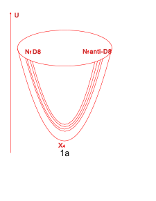
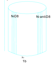
Figure 1: The dominant configurations of the D8 and anti-D8 probe branes in Sakai-Sugimoto model in deconfinement phase. (1a) indicates the chiral symmetry is broken, and (1b) signifies the chiral symmetry is restored. If D8 and $\overline{D8}$ are separated by a distance L at infinity, for $T>0.154/L$, (1b) is the dominant phase, for $T_{d}<T<0.154/L$, (1a) is the dominant phase

3 Calculation of the momentum diffusion coefficient

3.1 Preliminaries

In [9, 10] the authors obtain the transverse momentum diffusion coefficient in the following way. Firstly, by analogy to classical theory for Brownian motion, they propose that

$$\kappa_{T}=\frac{1}{2}\int_{-\infty}^{\infty}dt\,\langle F(t)F(0)+F(t)F(0)\rangle,$$ (7)

where $F(t)$ is the transverse stochastic force acting on the probe quark. In $\mathcal{N}=4$ SYM, it takes the form

$$F(t)=\int d^{3}\vec{x}Q^{{\dagger}}(t,\vec{x})T^{a}Q(t,\vec{x})E^{a},$$ (8)

where $E^{a}$ is the field strength supplied by vector gauge fields and six scalar fields. We can define the Wightman correlation function and the Feynman correlation function about $F(t)$, they are

$$G(t)=\frac{1}{2}\langle F(t)F(0)+F(t)F(0)\rangle,$$ (9)

$$G_{F}(t)=-i\langle{{\rm T}F(t)F(0)}\rangle.$$ (10)

And there is a relation between them in frequency space,

$$G(\omega)=-{\rm Im}G_{F}(\omega).$$ (11)

So, Eq. (7) can be changed into

$$\kappa_{T}=\lim_{\omega\to 0}G(\omega)=-\lim_{\omega\to 0}{\rm Im}G_{F}(\omega).$$ (12)

The $\langle\leavevmode\nobreak\ \leavevmode\nobreak\ \leavevmode\nobreak\ \rangle$ denotes an average in the states which are composed of SYM and a moving quark. Using Wigner distribution function in QCD kinetic theory, the generating functional of the above correlation functions can be written as the VEV of a Wilson loop. This loop is a closed contour in the complex time plane, specially, its $x$ component should satisfy $x=x_{0}+v(t_{c}-t_{c_{0}})$ and $y$ component is equal to $\delta$$y_{1}(t_{c})$ when $t_{c}$ lies on the real time axis, $\delta$$y_{2}(t_{c})$ when $t_{c}$ lies below the real time axis. This choice is determined by that the probe quark is traveling in $x$ direction with velocity $v$, and $\delta$$y_{1}(t)$, $\delta$$y_{2}(t)$ are the fluctuations of quark’s displacement in transverse direction acting as external sources coupling to the transverse stochastic force.

The authors of paper [8, 9, 10] evaluate the VEV of the Wilson loop via AdS/CFT correspondence in $AdS_{5}$-Schwarzschild background, by finding out a string’s classical action, requiring that the boundary of string’s world-sheet is the Wilson loop. This is to say

$$\frac{1}{e^{iS_{NG}[0,0]}}e^{iS_{NG}[\delta y_{1},\delta y_{2}]}=\frac{1}{\langle W[0,0]\rangle}\,\langle W[\delta y_{1},\delta y_{2}]\rangle.$$ (13)

The closed time contour corresponds to the two boundaries of global $AdS_{5}$-Schwarzschild space and the string stretches between the two boundaries. Finally, they obtain

$${}\kappa_{T}=\sqrt{\gamma\lambda}T^{3}\pi\,,$$ (14)

when $v\rightarrow 0,\gamma\rightarrow 1$, $\kappa_{T}$ and the drag coefficient [21, 22] satisfy the Einstein relation.

3.2 Calculation of the $\kappa_{T}$ in S-S model

In S-S model, $E^{a}$ appearing in the stochastic force term (8) should also include the contribution from K-K modes with mass of the order of QGP temperature. We will use the deconfinement phase background (2). For convenience, we use $u_{T}$ to scale dimensional coordinates and other parameter.

$$ds^{2} =u_{T}^{2} \left(\frac{u}{R}\right)^{3/2}\left[-f(u)dt^{2}+\delta_{ij}dx^{i}dx^{j}+dx_{4}^{2}\right]+\left(\frac{R}{u}\right)^{3/2}\left[u^{2}d\Omega_{4}^{2}+\frac{du^{2}}{f(u)}\right],$$ (15)

where $R=\frac{R_{D_{4}}}{u_{T}}$, $f(u)=1-\frac{1}{u^{3}}$, and now all the coordinates are dimensionless. Since this background is spherically symmetric , to define its Kruskal coordinates is a routine. They are

$$U=e^{-2\nu_{+}},\quad V=e^{2\nu_{-}},$$ (16)

where

$$\nu_{+}\equiv t+z_{*},\quad\nu_{-}=t-z_{*},$$ (17)

and

$$z_{*}=\int^{u}\frac{du}{f(u)(\frac{u}{R})^{3/2}}\leavevmode\nobreak\ \leavevmode\nobreak\ \leavevmode\nobreak\ .$$ (18)

But we only need the near horizon behavior of the Kruskal coordinates. In the near horizon limit, the metric becomes

$$ds^{2}\sim 3u_{T}^{2}R^{-3/2}\left[-(1-\frac{1}{u})dt^{2}+\frac{R^{3}du^{2}}{9(1-\frac{1}{u})}\right]+u_{T}^{2}R^{-3/2}\left[\delta_{ij}dx^{i}dx^{j}+dx_{4}^{2}+R^{3}d\Omega_{4}^{2}\right].$$ (19)

If we define

$$\rho=\frac{R^{3/2}}{3}u,\quad 2M=\frac{R^{3/2}}{3}\leavevmode\nobreak\ \leavevmode\nobreak\ \leavevmode\nobreak\ ,$$ (20)

then this metric looks like Schwarzschild metric

$$ds^{2}\sim 3u_{T}^{2}R^{-3/2}\left[-(1-\frac{2M}{\rho})dt^{2}+\frac{d\rho^{2}}{1-2M/\rho}\right]+u_{T}^{2}R^{-3/2}\left[\delta_{ij}dx^{i}dx^{j}+dx_{4}^{2}+R^{3}d\Omega_{4}^{2}\right]\leavevmode\nobreak\ .$$ (21)

The near horizon Kruskal coordinates are the same as in the Schwarzschild metric,

$$U=-4Me^{-(t-r_{*})/4M},\quad V=4Me^{(t-r_{*})/4M}\leavevmode\nobreak\ ,$$ (22)

where

$$r^{*}=\rho+2M\ln|\rho/2M-1|.$$ (23)

In background (15) the string configuration with a constant velocity $v$ in $x^{1}$ direction is as [19]

$$x^{1}(t,u)=vt+\frac{vR^{3/2}}{3}\ln\frac{|u-1|}{\sqrt{u^{2}+u+1}}-\frac{vR^{3/2}}{\sqrt{3}}\arctan\frac{2u+1}{\sqrt{3}}\leavevmode\nobreak\ .$$ (24)

with other coordinates kept constant, where we have chosen the $t$ and $u$ coordinates to parameterize the string world-sheet. So the string configuration with a perturbation $\delta y(t,u)$ in the $x^{2}$ direction should be

$$x^{\mu}=(t,x^{1}(t,u),\delta y(t,u),u,\rm const).$$ (25)

If we insert $x^{\mu}$ into metric (15), we get the induced metric on the world-sheet,

$$ds_{induced}^{2}=\left(\frac{u}{R_{D4}}\right)^{3/2}\left[-(\frac{1}{\gamma^{2}}-\frac{u_{T}^{3}}{u^{3}})dt^{2}+(\frac{R_{D4}}{u})^{3}\frac{1-\frac{u^{3}_{T}}{\gamma^{2}u^{3}}du^{2}}{(1-\frac{u^{3}_{T}}{u^{3}})^{2}}+\frac{2v^{2}R_{D4}^{3/2}u^{3/2}_{T}dtdu}{u^{3}(1-\frac{u^{3}_{T}}{u^{3}})}+d\delta y(t,u)^{2}\right]\leavevmode\nobreak\ ,$$ (26)

where we have restored the dimension of the coordinates, and $\gamma$ is the Lorentz factor. This metric can be simplified by performing coordinate transformation,

$$\bar{t} =\frac{t}{\gamma}+\frac{R_{D4}^{3/2}}{3\gamma u^{1/2}_{T}}\left[\ln\frac{p-1}{\sqrt{p^{2}+p+1}}\right.$$ (27)

$$\qquad\left.-\sqrt{3}\arctan\frac{2p+1}{\sqrt{3}}-\gamma^{2/3}\ln\frac{q-1}{\sqrt{q^{2}+q+1}}+\gamma^{2/3}\sqrt{3}\arctan\frac{2q+1}{\sqrt{3}}\right],$$

$$\bar{u}=u,$$ (28)

where $p=\frac{u}{u_{T}}$, $q=\frac{u}{\gamma^{2/3}u_{T}}$, then the metric becomes

$$ds_{induced}^{2}=\left(\frac{\bar{u}}{R_{D4}}\right)^{3/2}\left[-(1-\frac{\gamma^{2}u_{T}^{3}}{\bar{u}^{3}})d\bar{t}^{2}+\frac{(\frac{R_{D4}}{\bar{u}})^{3}d\bar{u}^{2}}{1-\frac{\gamma^{2}u^{3}_{T}}{\bar{u}^{3}}}+d\delta y(\bar{t},\bar{u})^{2}\right].$$ (29)

Now we define $\hat{t}\gamma^{2/3}u_{T}=\bar{t}$, $\hat{u}\gamma^{2/3}u_{T}=\bar{u}$,  $\delta\hat{y}(\hat{t},\hat{u})\gamma^{2/3}u_{T}=\delta y(\bar{t},\bar{u})$, $\hat{R}\gamma^{2/3}u_{T}=R_{D4}$, then the metric looks like the original one (15),

$$ds^{2}=(\gamma^{2/3}u_{T})^{2}(\hat{R}/\hat{u})^{-3/2}\left[-f(\hat{u})d\hat{t}^{2}+(\frac{\hat{R}}{\hat{u}})^{3}\frac{d\hat{u}^{2}}{f(\hat{u})}+d\delta\hat{y}(\hat{t},\hat{u})^{2}\right]\leavevmode\nobreak\ ,$$ (30)

with $u_{T}\rightarrow\gamma^{2/3}u_{T}$, $R\rightarrow\hat{R}$. A compelling characteristic is that from the point of view of string world-sheet, the horizon shifts to $\hat{u}=1$, or $u$=$\gamma^{2/3}$. This new horizon is usually called the world-sheet horizon. The near horizon Kruskal coordinates can be defined by

$$\hat{U}=-4\hat{M}e^{-(\hat{t}-\hat{r}_{*})/4\hat{M}},\quad\hat{V}=4\hat{M}e^{(\hat{t}-\hat{r}_{*})/4\hat{M}}\leavevmode\nobreak\ ,$$ (31)

where

$$\hat{\rho}=\frac{\hat{R}^{3/2}}{3}\hat{u},\quad 2\hat{M}=\frac{\hat{R}^{3/2}}{3}\leavevmode\nobreak\ ,$$ (32)

$$\hat{r}^{*}=\hat{\rho}+2\hat{M}\ln|\hat{\rho}/2\hat{M}-1|\leavevmode\nobreak\ .$$ (33)

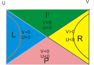
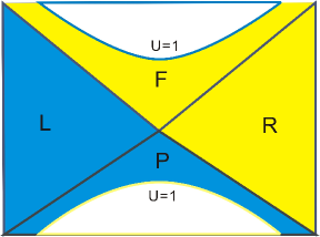
Figure 2: The left figure is the space-time Penrose diagram in Kruskal coordinates. The right figure is the string world-sheet Penrose diagram in world-sheet Kruskal coordinates. The regions with yellow color in two figures, represent the same zone in space-time, so are the blue regions. The hyperbolas in the space-time Penrose diagram correspond to the world-sheet horizon.

In Figure 2, in the R patch of world-sheet Kruskal plane, the action of the small fluctuations $\delta\hat{y}(\hat{t},\hat{u})$ is derived from the Nambu-Goto action

$$S=\frac{(\gamma^{2/3}u_{T})^{2}}{2\pi\alpha^{\prime}}\int d\hat{t}d\hat{u}\sqrt{1-f^{-1}(\hat{u})\delta\dot{\hat{y}}^{2}+f(\hat{u})\frac{\hat{u}^{3}}{\hat{R}^{3}}\delta\hat{y}^{\prime 2}},$$ (34)

where “dot” denotes $\partial_{\hat{t}}$, “prime” denotes $\partial_{\hat{u}}$. Because $\delta\hat{y}$ is small, we can expand action around $\delta\hat{y}$ = 0, and keep up to the second order of $\delta\hat{y}$.

$$S=\frac{(\gamma^{2/3}u_{T})^{2}}{2\pi\alpha^{\prime}}\int d\hat{t}d\hat{u}(1-\frac{1}{2}f^{-1}(\hat{u})\delta\dot{\hat{y}}^{2}+\frac{1}{2}f(\hat{u})\frac{\hat{u}^{3}}{\hat{R}^{3}}\delta\hat{y}^{\prime 2}).$$ (35)

Note that the infinite part of the action is subtracted since it appears in the numerator and denominator of Eq. (13). To solve fluctuation $\delta\hat{y}$ , we define

$$\delta\hat{y}(\hat{t},\hat{u})=\int\frac{d\hat{\omega}}{2\pi}\exp^{-i\hat{\omega}\hat{t}}\hat{y}(\hat{\omega})\hat{Y}(\hat{u},\hat{\omega}),$$ (36)

where we have chosen to normalize $\hat{Y}(\hat{u}=\infty,\hat{\omega})$ = 1, because $\hat{y}(\hat{\omega})$ is the Fourier transformation of the boundary value of $\delta\hat{y}(\hat{t},\hat{u})$. The Euler-Lagrange equation of small string fluctuations can be written as

$$\partial^{2}_{\hat{u}}\hat{Y}_{\hat{\omega}}+\frac{3\hat{u}^{2}}{\hat{u}^{3}-1}\partial_{\hat{u}}\hat{Y}_{\hat{\omega}}+\frac{\hat{\omega}^{2}\hat{u^{3}}\hat{R}^{3}}{(\hat{u}^{3}-1)^{2}}\hat{Y}_{\hat{\omega}}=0.$$ (37)

This equation is solved by

$$\hat{Y}(\hat{u},\hat{\omega})=(1-\frac{1}{\hat{u}^{3}})^{-i\frac{\hat{\omega}\hat{R}^{3/2}}{3}}F(\hat{\omega},\hat{u}),$$ (38)

where $F(\hat{\omega},\hat{u})$ is a regular function of $\hat{u}$. $(1-\frac{1}{\hat{u}^{3}})^{-i\frac{\hat{\omega}\hat{R}^{3/2}}{3}}$ corresponds to in-falling fluctuation in the world-sheet horizon $\hat{u}=1$. The complex conjugate of this expression is also a solution of the differential equation (37) and corresponds to out-going fluctuation in the horizon.

Now, we have obtained the solution in the R patch of world-sheet Kruskal plane representing the right part of the R patch of the space-time Kruskal plane. The right and left parts in the R patch are separated by the curve $u=\gamma^{2/3}$, as in Figure 2. But in order to use gauge/string duality to obtain the generating functional of the Feynman correlation function, we need to know the solution defined in the whole Kruskal plane of space-time. To this goal, we will extend the solution in the right half of the R patch into other parts of Kruskal plane one by one. Firstly, we should extend the solution into the whole R patch of space-time Kruskal plane. In other words, this amounts to extending the solution from R patch of world-sheet Kruskal plane to the R and F parts of world-sheet Kruskal plane. In terms of near horizon Kruskal coordinates, the in-falling and out-going solutions in R patch of world-sheet Kruskal plane behave as

$$\mbox{in-falling:}\leavevmode\nobreak\ \leavevmode\nobreak\ \leavevmode\nobreak\ \leavevmode\nobreak\ e^{-i\hat{\omega}\hat{t}}\hat{Y}(\hat{\omega},\hat{u})\sim e^{-4i\hat{\omega}\hat{M}\ln\hat{V}},$$ (39)

$$\mbox{out-going:}\leavevmode\nobreak\ \leavevmode\nobreak\ \leavevmode\nobreak\ \leavevmode\nobreak\ e^{-i\hat{\omega}\hat{t}}\hat{Y}^{*}(\hat{\omega},\hat{u})\sim e^{4i\hat{\omega}\hat{M}\ln-\hat{U}}.$$ (40)

Because the Kruskal coordinates are global, actually, in the F patch of world-sheet Kruskal plane, near world-sheet horizon, we can also write down these two solutions as

$$\mbox{in-falling:}\leavevmode\nobreak\ \leavevmode\nobreak\ \leavevmode\nobreak\ \leavevmode\nobreak\ e^{-i\hat{\omega}\hat{t}}\hat{Y}(\hat{\omega},\hat{u})\sim e^{-4i\hat{\omega}\hat{M}\ln\hat{V}},$$ (41)

$$\mbox{ out-going:}\leavevmode\nobreak\ \leavevmode\nobreak\ \leavevmode\nobreak\ \leavevmode\nobreak\ e^{-i\hat{\omega}\hat{t}}\hat{Y}^{*}(\hat{\omega},\hat{u})\sim e^{4i\hat{\omega}\hat{M}\ln\hat{U}}.$$ (42)

From above expressions, in the F patch of world-sheet Kruskal plane, we see that the in-falling solution is still effective, because $\hat{V}>0$, but $\hat{U}$ changes sign. So we will do an analytic extension for the out-going solution to make it an solution in the R and F patches of the world sheet Kruskal plane. Following Herzog and Son’s prescription [23], the out-going solution should cross the horizon from the upper half of complex $\hat{U}$, this results in that the out-going wave should picks up a factor $e^{4\pi\hat{\omega}\hat{M}}$. Physically, this indicates that the out-going wave should be purely negative-frequency. We can repeat this process in the P and L patches. Having done this, the out-going solution picks up a factor $e^{-4\pi\hat{\omega}\hat{M}}$. Now, we have solutions defined in $\hat{V}>0$, $\hat{V}<0$ parts of the world-sheet Kruskal plane. As we have demenstrated previously, the R and F patches of the world sheet Kruskal plane represent the R patch of the space-time Kruskal plane. The L and P patches of the world sheet Kruskal plane represent the L patch of the space-time Kruskal plane. So we know how these solutions behave in the R and L patches of the space-time Kruskal plane respectively. Near space-time horizon, in terms of the space-time near horizon Kruskal coordinates, in the R patch of the space-time

$$\mbox{in-falling:}\leavevmode\nobreak\ \leavevmode\nobreak\ \leavevmode\nobreak\ \leavevmode\nobreak\ e^{-i\hat{\omega}\hat{t}}\hat{Y}(\hat{\omega},\hat{u})\sim e^{-4i\omega M\ln V},$$ (43)

$$\mbox{out-going:}\leavevmode\nobreak\ \leavevmode\nobreak\ \leavevmode\nobreak\ \leavevmode\nobreak\ e^{4\pi\hat{\omega}\hat{M}}e^{-i\hat{\omega}\hat{t}}\hat{Y}^{*}(\hat{\omega},\hat{u})\sim e^{4\pi\hat{\omega}\hat{M}}e^{-4i\omega M\ln V}.$$ (44)

in the L patch of the space-time

$$\mbox{in-falling:}\leavevmode\nobreak\ \leavevmode\nobreak\ \leavevmode\nobreak\ \leavevmode\nobreak\ e^{-i\hat{\omega}\hat{t}}\hat{Y}(\hat{\omega},\hat{u})\sim e^{-4i\omega M\ln(-V)},$$ (45)

$$\mbox{out-going:}\leavevmode\nobreak\ \leavevmode\nobreak\ \leavevmode\nobreak\ \leavevmode\nobreak\ e^{-4\pi\hat{\omega}\hat{M}}e^{-i\hat{\omega}\hat{t}}\hat{Y}^{*}(\hat{\omega},\hat{u})\sim e^{-4\pi\hat{\omega}\hat{M}}e^{-4i\omega M\ln(-V)}.$$ (46)

These expressions tell us that in the point of view of space-time, the in-falling and out-going solutions in the world-sheet are both in-falling waves. Moreover, the R patch solutions can be interpreted as the solution in both the R and F patches. The L patch solutions can be interpreted as the solution in both the L and P patches, because $V>0$ in both the R and F patches; $V<0$ in both the L and P patches. So far, we have obtained the solution defined in the whole $V>0$ part of Kruskal plane, and the solution defined in the whole $V<0$ part of Kruskal plane. They can be deduced from the following four different solutions defined in R and L patches.

$${\hat{y}}_{R,\leavevmode\nobreak\ i}=\left\{\begin{array}[]{ll}e^{-i{\hat{\omega}}{\hat{t}}}{\hat{Y}}({\hat{\omega}},{\hat{u}})&\mbox{in R}\\ 0&\mbox{in L}\end{array}\right.\;\;\;\;\;\;\;\;\;\;{\hat{y}}_{L,\leavevmode\nobreak\ i}=\left\{\begin{array}[]{ll}0&\mbox{in R}\\ e^{-i{\hat{\omega}}{\hat{t}}}{\hat{Y}}({\hat{\omega}},{\hat{u}})&\mbox{in L}\end{array}\right.\ ,$$ (47)

$${\hat{y}}_{R,\leavevmode\nobreak\ o}=\left\{\begin{array}[]{ll}e^{-i{\hat{\omega}}{\hat{t}}}{\hat{Y}}^{*}({\hat{\omega}},{\hat{u}})&\mbox{in R}\\ 0&\mbox{in L}\end{array}\right.\;\;\;\;\;\;\;\;\;\;{\hat{y}}_{L,\leavevmode\nobreak\ o}=\left\{\begin{array}[]{ll}0&\mbox{in R}\\ e^{-i{\hat{\omega}}{\hat{t}}}{\hat{Y}}^{*}({\hat{\omega}},{\hat{u}})&\mbox{in L}\end{array}\right.\,.$$ (48)

Following the Herzog and Son prescription [23], we look for linear combinations of these expressions that, close to the horizon, are analytic in the lower half of the complex V plane. Physically, this means that the in-falling wave should be purely positive-frequency. With this requiriement, the two linearly independent combination are:

$${\hat{y}}_{o}={\hat{y}}_{R,\leavevmode\nobreak\ o}+\alpha_{o}{\hat{y}}_{L,\leavevmode\nobreak\ o}\,,\\ \leavevmode\nobreak\ \leavevmode\nobreak\ \leavevmode\nobreak\ \leavevmode\nobreak\ {\hat{y}}_{i}={\hat{y}}_{R,\leavevmode\nobreak\ i}+\alpha_{i}{\hat{y}}_{L,\leavevmode\nobreak\ i}\,.$$ (49)

where the $\alpha_{o}$ and $\alpha_{i}$ can be determined from the near horizon behaviors of these solutions Eqs. (43), (44), (45) and (45)

$$\alpha_{o}=e^{8\pi{\hat{\omega}}{\hat{M}}}e^{-4\pi\omega M},$$ (50)

$$\alpha_{i}=e^{-4\pi\omega M}.$$ (51)

These two solutions are used as basis for the linearized string fluctuations defined over the full (AdS) Kruskal plane

$${\hat{y}}({\hat{t}},{\hat{u}})=\int\frac{d{\hat{\omega}}}{2\pi}\left(a(\omega){\hat{y}}_{o}(\omega)+b(\omega){\hat{y}}_{i}(\omega)\right)\,.$$ (52)

The coefficients $a({\hat{\omega}}),\leavevmode\nobreak\ b({\hat{\omega}})$ can be determined by the boundary values of the solutions. Because we have

$${\hat{y}}({\hat{t}},{\hat{u}}=\infty)\big{|}_{R} = \int\frac{d{\hat{\omega}}}{2\pi}e^{-i{\hat{\omega}}{\hat{t}}}{\hat{y}}_{1}({\hat{\omega}})\,,$$ (53)

$${\hat{y}}({\hat{t}},{\hat{u}}=\infty)\big{|}_{L} = \int\frac{d{\hat{\omega}}}{2\pi}e^{-i{\hat{\omega}}{\hat{t}}}{\hat{y}}_{2}({\hat{\omega}})\,.$$ (54)

We obtain

$$a({\hat{\omega}})=\hat{n}(-{\hat{y}}_{1}({\hat{\omega}})+e^{4\pi\omega M}{\hat{y}}_{2}({\hat{\omega}})),$$ (55)

$$b({\hat{\omega}})=\hat{n}(e^{8\pi{\hat{\omega}}{\hat{M}}}{\hat{y}}_{1}({\hat{\omega}})-e^{4\pi\omega M}{\hat{y}}_{2}({\hat{\omega}})).$$ (56)

where $\hat{n}=1/(e^{8\pi{\hat{\omega}}{\hat{M}}}-1)$. Now we compute the boundary action in terms of the string solution: In $({\hat{t}},{\hat{u}})$ coordinates

$$S_{B}=\frac{(\gamma^{2/3}u_{T})^{2}}{2\pi\alpha^{\prime}}\left[\int_{R}\frac{d\hat{\omega}}{2\pi}f({\hat{u}})\frac{{\hat{u}}^{3}}{\hat{R}^{3}}{\hat{y}}(-\hat{\omega},\hat{u})\partial_{\hat{u}}{\hat{y}}(\hat{\omega},\hat{u})-\int_{L}\frac{d\hat{\omega}}{2\pi}f({\hat{u}})\frac{{\hat{u}}^{3}}{\hat{R}^{3}}{\hat{y}}(-\hat{\omega},\hat{u})\partial_{\hat{u}}{\hat{y}}(\hat{\omega},\hat{u})\right].\,$$ (57)

Notice that ${\hat{\omega}}=\gamma\omega$, ${\hat{y}}_{1}({\hat{\omega}})=\gamma^{-1}y_{1}(\omega)$, ${\hat{y}}_{2}({\hat{\omega}})=\gamma^{-1}y_{2}(\omega)$, and using Eqs. (47), (48), (50), (51), (55), (56) and (52), this action can be expressed as

$$S_{B}=\frac{(\gamma^{2/3}u_{T})^{2}}{2\pi\alpha^{\prime}\gamma}\int\frac{d\omega}{2\pi}\left.\Big{[}\right.$$ (58)

$$y_{1}(-\omega)y_{1}(\omega)\left.(({\hat{n}}+1)f({\hat{u}})\frac{{\hat{u}}^{3}}{\hat{R}^{3}}{\hat{Y}}^{*}(-\hat{\omega},\hat{u})\partial_{\hat{u}}{\hat{Y}}(\hat{\omega},\hat{u})-{\hat{n}}f({\hat{u}})\frac{{\hat{u}}^{3}}{\hat{R}^{3}}{\hat{Y}}(-\hat{\omega},\hat{u})\partial_{\hat{u}}{\hat{Y}}^{*}(\hat{\omega},\hat{u})\right)$$

$$+y_{1}(-\omega)y_{2}(\omega)e^{\pi\omega/2}{\hat{n}}\left.(-f({\hat{u}})\frac{{\hat{u}}^{3}}{\hat{R}^{3}}{\hat{Y}}^{*}(-\hat{\omega},\hat{u})\partial_{\hat{u}}{\hat{Y}}(\hat{\omega},\hat{u})+f({\hat{u}})\frac{{\hat{u}}^{3}}{\hat{R}^{3}}{\hat{Y}}(-\hat{\omega},\hat{u})\partial_{\hat{u}}{\hat{Y}}^{*}(\hat{\omega},\hat{u})\right)$$

$$+y_{2}(-\omega)y_{1}(\omega)e^{-\pi\omega/2}(1+{\hat{n}})\left.(-f({\hat{u}})\frac{{\hat{u}}^{3}}{\hat{R}^{3}}{\hat{Y}}^{*}(-\hat{\omega},\hat{u})\partial_{\hat{u}}{\hat{Y}}(\hat{\omega},\hat{u})+f({\hat{u}})\frac{{\hat{u}}^{3}}{\hat{R}^{3}}{\hat{Y}}(-\hat{\omega},\hat{u})\partial_{\hat{u}}{\hat{Y}}^{*}(\hat{\omega},\hat{u})\right)$$

$$+y_{2}(-\omega)y_{2}(\omega)\left.({\hat{n}}f({\hat{u}})\frac{{\hat{u}}^{3}}{\hat{R}^{3}}{\hat{Y}}^{*}(-\hat{\omega},\hat{u})\partial_{\hat{u}}{\hat{Y}}(\hat{\omega},\hat{u})-({\hat{n}}+1)f({\hat{u}})\frac{{\hat{u}}^{3}}{\hat{R}^{3}}{\hat{Y}}(-\hat{\omega},\hat{u})\partial_{\hat{u}}{\hat{Y}}^{*}(\hat{\omega},\hat{u})\right)\Big{]}\big{|}_{u\rightarrow+\infty}.$$

From this expression we can read off the Feynman correlation by taking derivatives with respect to $y_{1}(-\omega)$, $y_{1}(\omega)$.

$$G_{F}(\omega)=\frac{1}{2\pi\alpha^{\prime}\gamma\gamma^{2/3}u_{T}}[{({\hat{n}}+1)f({\hat{u}})\frac{{\hat{u}}^{3}}{{\hat{R}}^{3}}{\hat{Y}}^{*}\partial_{{\hat{u}}}{\hat{Y}}({\hat{\omega}},{\hat{u}})-{\hat{n}}f({\hat{u}})\frac{{\hat{u}}^{3}}{{\hat{R}}^{3}}{\hat{Y}}\partial_{{\hat{u}}}{\hat{Y}}^{*}({\hat{\omega}},{\hat{u}})}]\big{|}_{{\hat{u}}\rightarrow\infty},$$ (59)

where we have restored physical dimension of $G_{F}$. When ${\hat{\omega}}\rightarrow 0$ we can expand ${\hat{Y}}({\hat{\omega}},{\hat{u}})$ in a power series in ${\hat{\omega}}$ and solve order by order

$${\hat{Y}}({\hat{\omega}},{\hat{u}}) =(1-\frac{1}{{\hat{u}}^{3}})^{-2i{\hat{M}}{\hat{\omega}}}\left[1-2i{\hat{M}}{\hat{\omega}}(3\ln({\hat{u}}/\sqrt{{\hat{u}}^{2}+{\hat{u}}+1})\right.$$ (60)

$$\qquad\left.-\sqrt{3}\arctan(2{\hat{u}}/\sqrt{3}+1/\sqrt{3})+\frac{\sqrt{3}\pi}{2})+{\cal O}({\hat{\omega}}^{2})\right].$$

So

$$\kappa_{T}=-\lim_{\omega\to 0}{\rm Im}G_{F}(\omega)=\frac{3\gamma^{1/3}u_{T}^{2}}{4\pi^{2}\alpha^{{}^{\prime}}R_{D4}^{3}},$$ (61)

where we have used ${\hat{R}}^{3}=\gamma^{-2}R^{3}$. Using the parameter relation between string theory and gauge theory, we obtain

$$\kappa_{T}=\frac{16\sqrt{2}\pi}{27}\frac{\gamma^{1/3}\lambda T^{4}}{T_{d}},$$ (62)

where $\lambda$ is the the ’t Hooft coupling of YM, $g_{YM}^{2}N_{c}$. When $v\rightarrow 0$ if $\kappa_{T}$ and the drag coefficient which is often denoted as $\eta_{D}$ satisfy the Einstein relation, then the drag coefficient in S-S model should be

$$\eta_{D}=\frac{1}{2\pi\alpha^{\prime}M}(\frac{u_{T}}{R_{D4}})^{3/2}.$$ (63)

This is the result appearing in [19].

4 An estimation of $\hat{q}$ with respect to gluon energy loss in S-S model

4.1 The initial energy-momentum of gluon in S-S model

In [11], S. Gubser and his collaborators proposed a simple but interesting idea to estimate the jet quenching parameter ${\hat{q}}$, by computing how far an off-shell gluon propagates in the finite temperature $\mathcal{N}=4$ SYM before it loses all energy and resolves into the medium. Their estimation is mainly based on an extension of BDMPS formalism [24, 25, 26] from light-like parton to time-like parton, which is to replace the light cone distance $L^{-}$, by $\sqrt{2}\Delta x$, where $\Delta x$ is the parton’s in-medium space distance, often called penetration length. In short, this is

$$\Delta E=\frac{1}{4}\alpha_{s}C_{R}{\hat{q}}\frac{L^{-2}}{2}\rightarrow\Delta E=\frac{1}{4}\alpha_{s}C_{R}{\hat{q}}\Delta x^{2},$$ (64)

and

$${\hat{q}}=\frac{4\Delta E}{\alpha_{s}C_{R}\Delta x^{2}}.$$ (65)

In above expressions, $\alpha_{s}$ is the strong coupling constant, and $C_{R}$ is the color group $SU(N)$ Casimir $C_{2}(R)$ evaluated in the parton’s representation, for gluon $C_{R}$=N. Although this is not an exact calculation about ${\hat{q}}$, it has a striking virtue appealing to us, that is their result ${\hat{q}}\sim 21{\rm GeV^{2}}/{\rm fm}$ lies within the $3\sigma$ range of averaged ${\hat{q}}$ [27], while other people’s result [6] fails. The $3\sigma$ range of averaged ${\hat{q}}$ is

$$7\frac{\rm GeV^{2}}{\rm fm}\lesssim\langle\hat{q}\rangle\lesssim 28\frac{\rm GeV^{2}}{\rm fm},$$ (66)

with lowest $\chi^{2}$ at $\langle\hat{q}\rangle\approx 13\,{\rm GeV}^{2}/{\rm fm}$. S-S model is also a holographic dual to QCD, so we can ask whether their method still has this advantage in S-S model.

To answer this question, we do the following estimate in S-S model. Firstly, we will introduce the following background for the simplicity of calculation,

$$ds^{2}=u^{2}_{T}(Ry)^{-\frac{3}{2}}[-(1-y^{3})dt^{2}+d\vec{x}^{2}+\frac{R^{3}dy^{2}}{y(1-y^{3})}].$$ (67)

This is obtained from the metric (15), by replacing $u$ with $\frac{1}{y}$ and letting $x_{4},\leavevmode\nobreak\ \Omega_{4}$ be constant. Following S. Gubser’s approach, a gluon is represented by a doubled string which rises from the horizon up to a minimum $y_{\rm UV}$, and then falls back down to the horizon as in Figure 3.

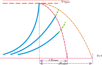
Figure 3: The blue line shows the shape of a doubled string which represents a gluon. The pink line and the orange line represent the world-sheet light signal’s trajectory and the massless particle’s trajectory we will introduce respectively. We will use these two trajectories to give an estimation of the range of gluon penetration length.

Required to be stable, the gluon’s initial state is constructed from the trailing string solution, the trailing string is a string moving with constant velocity in $x^{1}$ direction in the background (67), and its shape is

$$x^{1}(t) = vt+vR^{\frac{3}{2}}\left[\frac{\ln(1-y)}{(1-\alpha)(1-\beta)}+\frac{\ln(1-\beta y)}{(\alpha-1)(\alpha-\beta)}+\frac{\ln(1-\alpha y)}{(\beta-\alpha)(\beta-1)}\right]+$$ (68)

$$vR^{\frac{3}{2}}\left[\frac{\ln(1-\beta y)}{\alpha-\beta}-\frac{\ln(1-\alpha y)}{\alpha-\beta}\right].$$

This solution is equal to (24), $\alpha=e^{2\pi i/3}$ and $\beta$ is $\alpha$’s complex conjugate, we prefer this expression because of its convenience for following calculation. So, if we insist to use world-sheet coordinates $\sigma^{\alpha}=(t,y)$, initially, the induced metric on the world-sheet is

$$g_{\alpha\beta}=u_{T}^{2}(Ry)^{-\frac{3}{2}}\begin{pmatrix}-h+v^{2}&-v^{2}yR^{3/2}/h\\ -v^{2}yR^{3/2}/h&R^{3}(h+v^{2}-hv^{2})/h^{2}y\end{pmatrix},$$ (69)

where $h=1-y^{3}$. The world-sheet current density of energy-momentum

is

$$P^{\alpha}_{m}={1\over\pi\alpha^{\prime}h(1-v^{2})}\begin{pmatrix}-h-v^{2}+hv^{2}&v&0&0\\ -hv^{2}y^{2}R^{-3/2}&hvy^{2}R^{-3/2}&0&0\end{pmatrix},\$$ (70)

where m=(0, 1, 2, 3) corresponds to $(t,\vec{x})$. Usually, the related doubled string’s energy-momentum in these four dimensions is

$$p_{m}=\frac{1}{u_{T}}\int_{y_{\rm UV}}^{1}dy\,\sqrt{-g}P^{t}_{m}={u_{T}\over\pi\alpha^{\prime}}{1\over\sqrt{1-v^{2}}}\int_{y_{\rm UV}}^{1}{dy\over hy^{2}}\begin{pmatrix}-h-v^{2}+hv^{2}&v&0&0\end{pmatrix}.\$$ (71)

Because $\partial_{t}$, $\partial_{\vec{x}}$ is the Killing vectors, so $p_{m}$ can be identified with the four-momentum of the gluon in the boundary gauge theory. But we are also confronted with the problem appearing in $\mathcal{N}$=4 SYM: the energy-momentum has a logarithmic divergence at $y$=1. Gubser gives an explanation for the appearance of this kind of divergence: this divergence is due to the fact that, to form the shape of a trailing string needs infinitely long time, and during this period, infinite energy-momentum has been transferred from the string to the medium, but it is still contained in the right hand side of Eq. (71). So once this shape has been formed, the rest energy-momentum of the string should not include the energy-momentum transferred into the horizon. To make this subtraction, we compute

$$p^{\rm fixedx^{1}}_{m} =\frac{1}{u_{T}}\left.\int_{y_{\rm UV}}^{1}dy\,\sqrt{-g}[P^{t}_{m}-(\frac{\partial t}{\partial y})_{x_{1}}P^{y}_{m}\right.]$$ (72)

$$\left.=\frac{u_{T}}{\pi\alpha^{\prime}}(\frac{1}{y_{UV}}-1)(-1,v,0,0),\right.$$

where the subscript $x^{1}$ indicates that the above integral is carried out along the $x^{1}$=conctant contour in the ($t$,$y$) plane. With Green theorem and $P^{\alpha}_{m;\leavevmode\nobreak\ \alpha}$=0, it is not hard to prove the difference between (71) and (72) is the amount of energy-momentum we want to subtract from (71). Now, we can show to the reader that this gluon is a time-like one. This is obvious, since

$$E^{2}-\vec{P}^{2}=[\frac{u_{T}}{\pi\alpha^{\prime}}(\frac{1}{y_{UV}}-1)]^{2}>0.$$ (73)

4.2 Estimation of gluon penetration length

Since this doubled string’s tip does not attach to the boundary brane, this string will fall down toward horizon. At some moment, the tip will touch the horizon, from the beginning to this moment, the tip travels $\Delta x$ in $x^{1}$ direction. Generally, $\Delta x$ is function of $y_{\rm UV}$ and velocity $v$ or $\gamma$. For a fixed energy gluon, $\Delta x$ is function of $y_{\rm UV}$ or $v$, for example, we choose $\Delta x$=$\Delta x(v)$, then the maximum value of $\Delta x(v)$ with respect to $v$ can be interpreted as the penetration length of the gluon. Although, we know the initial shape of the doubled string, it is difficult to compute $\Delta x$ in terms of the EOM of string, not to mention $\Delta x_{\rm max}$. But with the methods proposed by Gubser, we can find out a lower and an upper bound for $\Delta x_{\rm max}$.

Firstly, we consider the lower bound. The initial shape of the doubled string can be interpreted as cutting the trailing string which attaches to the boundary brane, at $y=y_{\rm UV}$ at some time. Meanwhile, a light signal is emitted from the cut. Since the disturbance arising from cutting the string cannot propagate more quickly than light, the string will keep its shape where the light has not even arrived, as if we did not make such a cut. The displacement of light in $x^{1}$ direction, denoted as $\Delta x_{\rm low}$, should be the lower bound of $\Delta x$, then $\Delta x_{\rm low,\leavevmode\nobreak\ max}$ serves as the lower bound of $\Delta x_{\rm max}$. The trajectory of the light signal can be determined from the light-like tangent vector of world-sheet metric, which satisfies as $t$ increases, $y$ increases. There is only one light-like tangent vector field meeting this requirement. It is

$$l^{\alpha}=\begin{pmatrix}R^{\frac{3}{2}}[-\frac{v^{2}y}{h(h-v^{2})}+\frac{\sqrt{1-v^{2}}}{\sqrt{y}(h-v^{2})}]\\[3.0pt] 1\end{pmatrix}.$$ (74)

So the light signal’s trajectory is determined by

$$\frac{dt}{dy}=R^{\frac{3}{2}}[-\frac{v^{2}y}{h(h-v^{2})}+\frac{\sqrt{1-v^{2}}}{\sqrt{y}(h-v^{2})}].$$ (75)

Solving this differential equation, we obtain

$$t=R^{\frac{3}{2}}\gamma^{\frac{2}{3}}\left[\frac{2}{(1-\alpha)(1-\beta)}\ln(1+\gamma^{1/3}\sqrt{y})+\frac{1}{(\alpha-1)(\alpha-\beta)}\ln\frac{1+\beta\gamma^{1/3}\sqrt{y}}{1-\beta\gamma^{1/3}\sqrt{y}}\right]$$

$$+R^{\frac{3}{2}}\gamma^{\frac{2}{3}}\left(\frac{1}{(\beta-\alpha)(\beta-1)}\ln\frac{1+\alpha\gamma^{1/3}\sqrt{y}}{1-\alpha\gamma^{1/3}\sqrt{y}}\right)$$

$$-R^{\frac{3}{2}}\left[\frac{\ln(1-y)}{(1-\alpha)(1-\beta)}+\frac{\ln(1-\beta y)}{(\alpha-1)(\alpha-\beta)}+\frac{\ln(1-\alpha y)}{(\beta-\alpha)(\beta-1)}\right]$$

$$-R^{\frac{3}{2}}\left[\frac{\ln(1-\beta y)}{\alpha-\beta}-\frac{\ln(1-\alpha y)}{\alpha-\beta}\right]$$

$$R^{\frac{3}{2}}\gamma^{\frac{2}{3}}\left[\frac{\ln(1-\gamma^{2/3}\beta y)}{(\alpha-1)(\alpha-\beta)}+\frac{\ln(1-\gamma^{2/3}\alpha y)}{(\beta-\alpha)(\beta-1)}\right]$$

$$+R^{\frac{3}{2}}\gamma^{\frac{2}{3}}\left[\frac{\ln(1-\gamma^{2/3}\beta y)}{\alpha-\beta}-\frac{\ln(1-\gamma^{2/3}\alpha y)}{\alpha-\beta}\right],$$ (76)

where the $\alpha$ and $\beta$ are the same as Eq. (68). Plugging Eq. (4.2) into Eq. (68) we obtain the orbit

$$x^{1}(z)=u_{T}\frac{2}{3}vR^{\frac{3}{2}}\gamma^{\frac{2}{3}}[\ln(1+\gamma^{1/3}\sqrt{y})+\alpha\ln(1+\beta\gamma^{1/3}\sqrt{y})+\beta\ln(1+\alpha\gamma^{1/3}\sqrt{y})].$$ (77)

So

$$\Delta x_{\rm low}=x^{1}(1)-x^{1}(y_{UV}),$$ (78)

where we restore the physical dimension of $x^{1}$. For convenience, we define

$$\Delta\hat{x}_{\rm low}=\frac{\Delta x_{\rm low}}{u_{T}R^{\frac{3}{2}}},$$ (79)

$${\hat{E}}=\frac{\pi\alpha^{\prime}E}{u_{T}}.$$ (80)

Now we should find the maximum value of $\Delta\hat{x}_{\rm low}$ with a fixed ${\hat{E}}=\gamma(\frac{1}{y_{\rm UV}}-1)$. If we define

$$\xi=\gamma^{2/3}y_{UV},$$ (81)

then $\Delta\hat{x}_{\rm low}$ is a function of $\xi$. Usually, to find the maximum value of $\Delta\hat{x}(\xi)_{\rm low}$, we will first find a $\xi_{*}$ satisfying

$$\partial_{\xi}\Delta\hat{x}(\xi)_{\rm low,\leavevmode\nobreak\ \xi=\xi_{*}}=0.$$ (82)

But this is only the point making $\Delta\hat{x}(\xi)_{\rm low}$ a local maximum or minimum and may not be the global maximum or minimum. In fact, there is only one $\xi_{*}$ satisfying Eq. (82), and $\Delta\hat{x}(\xi_{*})_{\rm low}$ is the global maximum, this is supported by numerical result. When ${\hat{E}}\gg 1$, we find that $\xi_{*}$ can be expanded in terms of ${\hat{E}}^{\frac{1}{5}}$, it is

$$\xi_{*}=0.38036+0.207807{\hat{E}}^{-\frac{2}{5}}+0.07596{\hat{E}}^{-\frac{4}{5}}-0.781227{\hat{E}}^{-1}+{\cal O}(\hat{E}^{-6/5}).$$ (83)

And

$$\Delta\hat{x}_{\rm low,\leavevmode\nobreak\ max}=0.84423{\hat{E}}^{\frac{2}{5}}-0.80997+0.04178{\hat{E}}^{-\frac{2}{5}}+0.71431{\hat{E}}^{-\frac{3}{5}}+{\cal O}({\hat{E}}^{-\frac{4}{5}}).$$ (84)

We exhibit the comparison of analytic result and numeric result in Figure (4). We find that when ${\hat{E}}\gg 1$, the analytic result indeed matches the numeric result well.

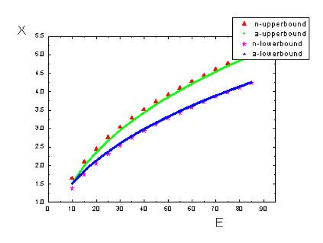
Figure 4: The triangles represent the numeric result of upper bound of penetration length, the stars represent the numeric result of the lower bound of penetration length, The two lines are the analytic results of the upper and lower bound of the penetration length for ${\hat{E}}\gg 1$ and their extrapolations to ${\hat{E}}$ not satisfying ${\hat{E}}\gg 1$.

Having found the lower bound of penetration length of the gluon, next, we shall look for the upper bound. To find the upper bound, we use the following picture. When the tip of the doubled string begins to fall toward the horizon, it happens that a light-like particle is projected from the tip with 5-dimension velocity proportional to the 5-dimension velocity of the tip. In other words, the massless particle’s trajectory is tangent to the tip’s trajectory at this point. The massless particle moves along the geodesic and will fall farther in $x^{1}$ direction than the tip, because the tip is also pulled by the rest of the string besides the gravity. So we can perceive the massless particle’s displacement in $x^{1}$ before it falls into the horizon, as the upper-bound of $\Delta x$ which we define before, here we denote this upper-bound by $\Delta x_{\rm upper}$. Then the maximum value of $\Delta x_{\rm upper}$ should be the upper-bound of $\Delta x_{\rm max}$, for fixed energy. To obtain $\Delta x_{\rm upper}$, we solve the EOM of the massless particle in the black hole background (67) with the initial condition required before. As we know, a massless particle can be described by the following action:

$$S=\frac{1}{2}\int d\eta[\frac{1}{e}G_{\mu\nu}\frac{dX^{\mu}}{d\eta}\frac{dX^{\nu}}{d\eta}],$$ (85)

where $e$ is a Lagrange multiplier, $G_{\mu\nu}$ is metric (67). In the following, let’s work in a gauge where $\eta=y$ and consider the trajectory of the form

$$X^{0}=X^{0}(y)\leavevmode\nobreak\ \leavevmode\nobreak\ \leavevmode\nobreak\ X^{1}=X^{1}(y)\leavevmode\nobreak\ \leavevmode\nobreak\ \leavevmode\nobreak\ X^{2}=X^{3}=0.$$ (86)

Then

$$S=\int dy\mathcal{L}\leavevmode\nobreak\ \leavevmode\nobreak\ \leavevmode\nobreak\ \mathcal{L}=\frac{u^{2}_{T}(Ry)^{-3/2}}{2e}(-h(X^{0^{\prime}})^{2}+(X^{1^{\prime}})^{2}+\frac{R^{3}}{yh}),$$ (87)

where prime denotes $d/dy$. Since the Lagrangian does not contain $X^{0}$, $X^{1}$ explicitly, we immediately form two conserved momenta

$$p_{0}=-\frac{u_{T}h(Ry)^{-3/2}X^{0^{\prime}}}{e}\leavevmode\nobreak\ \leavevmode\nobreak\ \leavevmode\nobreak\ \leavevmode\nobreak\ p_{1}=\frac{u_{T}(Ry)^{-3/2}X^{1^{\prime}}}{e}.$$ (88)

The equation of motion of $e$ is a constraint:

$$e=\pm\frac{u_{T}}{y^{2}\sqrt{p^{2}_{0}-hp^{2}_{1}}}.$$ (89)

Because of our metric signature, the -$p_{0}$ is energy, and should be positive, so $p_{0}$ is negative, for $X^{0^{\prime}}$ is positive, corresponding that the massless particle falls toward black hole, finally, we choose plus sign in (89) for the trajectory. Then the shape of the trajectories is determined by

$$\frac{dX^{1}}{dy}=X^{1^{\prime}}=\frac{ep_{1}(Ry)^{3/2}}{u_{T}}=-R^{3/2}\frac{p_{1}/p_{0}}{\sqrt{y}\sqrt{1-hp^{2}_{1}/p^{2}_{0}}}\leavevmode\nobreak\ ,$$ (90)

where $p_{1}/p_{0}$ is due to the initial condition, since $p_{1}$ and $p_{0}$ are conserved quantities. Because the tip of an open string or a doubled string must move at the speed of light, at the moment when the tip is formed, its 5-dimensional velocity should be proportional to $l^{\mu}|_{y=y_{\rm UV}}$, which is $l^{\alpha}\partial X^{\mu}/\partial\sigma^{\alpha}|_{y=y_{\rm UV}}$, satisfying $G_{\mu\nu}l^{\mu}l^{\nu}=0$. For $l^{\alpha}$’s definition, refer to (74). Then we can derive $p_{1}/p_{0}$

$$p_{1}/p_{0}=v\frac{\sqrt{1-v^{2}}-y^{3/2}_{UV}}{v^{2}y^{3/2}_{UV}-\sqrt{1-v^{2}}(1-y_{UV}^{3})}.$$ (91)

Now we calculate how far the massless particle propagates in the $X^{1}$ direction before falling into the horizon:

$$\Delta x_{\rm upper}=-R^{3/2}u_{T}\int^{1}_{y_{\rm UV}}dy\frac{p_{1}/p_{0}}{\sqrt{y}\sqrt{1-hp^{2}_{1}/p^{2}_{0}}}.$$ (92)

The maximum of $\Delta\hat{x}_{\rm upper}=\frac{\Delta x_{\rm upper}}{R^{3/2}u_{T}}$ for fixed ${\hat{E}}$ is depicted in the Figure 4. For ${\hat{E}}\gg 1$, using the same method as before, we find that

$$\xi_{*}=0.32141+0.13949{\hat{E}}^{-\frac{2}{5}}+0.03882{\hat{E}}^{-\frac{4}{5}}+{\cal O}({\hat{E}}^{-\frac{6}{5}})$$ (93)

$$\Delta\hat{x}_{\rm upper,max}=0.99033{\hat{E}}^{\frac{2}{5}}-0.79951+0.49157{\hat{E}}^{-\frac{2}{5}}+{\cal O}({\hat{E}}^{-\frac{4}{5}}).$$ (94)

At this moment, we should remind the reader that the analytic results do not match the numeric results as well as in the lower-bound case, the deviation may come from the approximate method we adopt to find out $\xi_{*}$.

So far, we have got two bounds of the gluon penetration length. Using these two bounds of penetration length to make a rough estimation of jet quenching parameter will be carried out in the discussion section.

5 Discussion

Following Gubser’s description, one is able to extract the jet quenching parameter from momentum diffusion constant $\kappa_{T}$, by

$${\hat{q}}_{B}=\frac{2\kappa_{T}}{v},$$ (95)

where “B” indicates Brownian motion, because we prefer to interpret it as part of the jet quenching parameter, this part is due to the Brownian motion effect. Since strongly coupled S-S model gauge field theory is different from QCD, there exists considerable uncertainty in how to translate the results calculated in S-S model into quantitative predictions in QCD.

To characterize this uncertainty, we recall that in $\mathcal{N}$=4 SYM, the optimum scheme is

$$T_{\mathcal{N}=4}=T_{QCD}/3^{1/4}=280/3^{1/4}\leavevmode\nobreak\ \leavevmode\nobreak\ \leavevmode\nobreak\ \leavevmode\nobreak\ g^{2}_{YM}N_{c}=5.5\leavevmode\nobreak\ .$$ (96)

The factor $3^{1/4}$ comes from the requirement that $\mathcal{N}$=4 SYM and QCD are compared at the same energy density. Similarly, we also require that the S-S model gauge theory and QCD are compared at the same energy density, and then choose the following scheme for S-S model:

$$T_{S-S}=T_{QCD}/\zeta=280{\rm MeV}/\zeta\leavevmode\nobreak\ \leavevmode\nobreak\ \leavevmode\nobreak\ T_{dQCD}=170{\rm MeV}\leavevmode\nobreak\ \leavevmode\nobreak\ \leavevmode\nobreak\ g^{2}_{YM}N_{c}=5.5\leavevmode\nobreak\ .$$ (97)

In above expressions,

$$\zeta=0.914\lambda^{1/6}(T_{QCD}/T_{d})^{1/3},$$ (98)

and in scheme (97), $\zeta\sim 1.43$. The explicit calculation of the parameter $\zeta$ will be given in appendix. We see that $\zeta$ is an increasing function of $T_{QCD}$. This is in accordance with our previous argument that as temperature increase, more K-K modes will become active, for their masses are in tower of $mT_{d}$, with $m=1,2\cdots$. Since more degrees of freedom contribute to the energy density, $\zeta$ must increase accordingly to keep the energy density of S-S model plasma equal with that of QCD plasma.

At this moment, we can calculate ${\hat{q}}_{B}$ as following,

$${\hat{q}}_{B}\sim 5.4{\rm GeV^{2}}/{\rm fm}\frac{\gamma^{1/3}}{\zeta^{3}v}=1.85{\rm GeV^{2}}/{\rm fm}\frac{\gamma^{1/3}}{v}.$$ (99)

For charm quark, $m_{c}$=1.4GeV, typical $p_{c}$=10GeV/c

$${\hat{q}}_{B}\sim 3.5{\rm GeV}^{2}/{\rm fm}.$$ (100)

This value of $\hat{q}_{B}$ is larger than Gubser’s result [10] ${\hat{q}}_{B}=1.4{\rm GeV}^{2}/{\rm fm}$ and Liu’s result [7] ${\hat{q}}=0.86{\rm GeV}^{2}/{\rm fm}$.

Now let us use the gluon penetration length to estimate the jet quenching parameter ${\hat{q}}$. Following (97), using BDMPS formalism and setting $\alpha_{s}=1/2$, we find

$$E=1.115{\hat{E}}{\rm GeV}\leavevmode\nobreak\ \leavevmode\nobreak\ \leavevmode\nobreak\ \leavevmode\nobreak\ \Delta x_{\rm max}({\hat{E}})=0.236\Delta\hat{x}({\hat{E}})_{\rm max}{\rm fm}$$ (101)

$${\hat{q}}=\frac{10.350\Delta{\hat{E}}}{\Delta\hat{x}({\hat{E}})_{\rm max}}{\rm GeV}^{2}/{\rm fm}.$$ (102)

Because $\Delta\hat{x}({\hat{E}})_{\rm lower\leavevmode\nobreak\ max}<\Delta\hat{x}({\hat{E}})_{\rm max}<\Delta\hat{x}({\hat{E}})_{\rm upper\leavevmode\nobreak\ max}$,

$$\frac{10.350\Delta{\hat{E}}}{\Delta\hat{x}({\hat{E}})_{\rm upper\leavevmode\nobreak\ max}}{\rm GeV}^{2}/{\rm fm}<{\hat{q}}<\frac{10.350\Delta{\hat{E}}}{\Delta\hat{x}({\hat{E}})_{\rm lower\leavevmode\nobreak\ max}}{\rm GeV}^{2}/{\rm fm}.$$ (103)

A representative range of energies for hard gluons in the QGP produced at RHIC, is $5{\rm GeV}<E<25{\rm GeV}$. When we make quantitative estimate of ${\hat{q}}$, we assume the energy of the gluon is 25GeV. The reason is that the higher the energy is, the longer the penetration length will be, and the ratio of radiative energy loss to collision energy loss should be larger, then $\Delta E$ appearing in BDMPS formalism may be roughly interpreted as the whole energy of the gluon, in short, in the following estimation, $\Delta E=25{\rm GeV}$. Inserting this value of $\Delta E$ into Eq. (103), we find

$$89{\rm GeV}^{2}/{\rm fm}<\hat{q}<106{\rm GeV}^{2}/{\rm fm}.$$ (104)

This result is much far away from the experimental result $7{\rm GeV}^{2}/{\rm fm}<{\hat{q}}<28{\rm GeV}^{2}/{\rm fm}$. The penetration length in S-S model seems too short, which may be a consequence of the extra hadronic degrees of freedom.

If we insist that scheme (97) should be the suitable one for comparing S-S model plasma with QCD plasma, the good performance of Gubser’s method in $\mathcal{N}$=4 SYM does not take place in S-S model. So there may be some unknown physical reasons that make Gubser’s method break down when applied to S-S model. It is also possible that the numeric range of $\hat{q}$ is similar to that of the experiment may be a coincidence, so we could not require it to be a feature belonging to all holographic QCD models. But even if this method can not be always used to estimate ${\hat{q}}$, the relation between gluon’s energy and penetration length may be still meaningful. However, we do not know how to relate it to experimental observables.

6 Appendix

In this section, we will exhibit a detailed calculation of the parameter $\zeta$ appearing in Eq. (97).

We recall that one of the first finite-temperature predictions of gauge/string duality is that of the thermodynamic potential of dual gauge theory in the strong coupling regime. The entropy is given by Bekenstein-Hawking formula $S=A/4G$, where $A$ is the area of the horizon, $G$ is the ten-dimensional Newton constant. To evaluate $A$, we cannot use string frame metric (15), but should use the metric in Einstein frame [28]. The metric in Einstein frame is obtained from multiplying the string metric (15) by $\sqrt{g_{s}e^{-\phi}}$, $\phi$ is the dilaton. The result is

$$ds^{2} = \left(\frac{u}{R_{D4}}\right)^{9/8}\left[-f(u)dt^{2}+\delta_{ij}dx^{i}dx^{j}+dx_{4}^{2}\right]+\left(\frac{R_{D4}}{u}\right)^{15/8}\left[u^{2}d\Omega_{4}^{2}+\frac{du^{2}}{f(u)}\right].$$ (105)

There are some parameter relations to be used, besides those given in (2)

$$g_{YM}^{2} = 4\pi^{2}g_{s}l_{s}T_{d}$$ (106)

$$G = 8\pi^{6}g_{s}^{2}l_{s}^{8},$$ (107)

where $T_{S-S}$ is the Hawking temperature of metric (15) and (105), $T_{d}$ is the critical temperature, $\lambda$ is the ’t Hooft coupling, $g_{s}$ and $l_{s}$ are string coupling and string length respectively. Using these relations, we obtain the entropy density of dual gauge theory by,

$$s_{S-S}=\frac{S}{V}=(\frac{2}{3})^{6}\pi^{2}\lambda N_{c}^{2}\frac{T_{S-S}^{5}}{T_{d}^{2}}.$$ (108)

Applying the following thermodynamic relations between entropy density $s$, pressure $P$ and free energy density $F$,

$$dP=-dF=sdT,$$ (109)

we find the pressure and energy density are

$$P_{S-S}=\frac{1}{6}Ts_{S-S},$$ (110)

$$\epsilon_{S-S}=\frac{5}{6}Ts_{S-S}.$$ (111)

It is straightforward to compute the sound speed of S-S plasma

$$v_{s}^{2}=\frac{1}{5}.$$ (112)

This value of sound speed implies that S-S plasma is not a kind of conformal fluid, for conformal fluid, $v_{s}^{2}$ must be 1/3. We recall that the energy density of QCD is

$$\epsilon_{QCD}=\frac{\pi^{2}}{8}N_{c}^{2}T_{QCD}^{4},$$ (113)

so we can deduce the relation between $T_{S-S}$ and $T_{QCD}$ by demanding that $\epsilon_{S-S}=\epsilon_{QCD}$,

$$T_{S-S}=T_{QCD}[0.914\lambda^{1/6}(T_{QCD}/T_{d})^{1/3}]^{-1}.$$ (114)

Then we can extract $\zeta$ from above expression

$$\zeta=0.914\lambda^{1/6}(T_{QCD}/T_{d})^{1/3}.$$ (115)

This is the Eq. (98).

7 Acknowledgements

I would like to thank M. Li, Y. Wang for useful discussions, and I thank X. Gao for helping me with typesetting, Y. Zhou for helping me revise my paper . Especially, I am grateful to Y. Wang for helping me learn using some softwares.

References

- [1] J. Adams(Star Collaboration) et. al., “Experimental and theoretical challenges in the search for the quark gluon plasma: The STAR collaboration’s critical assessment of the evidence from RHIC collisions”, Nucl. Phys. A757 (2005) 102–183, nucl-ex/0501009.
- [2] K. Adcox et. al., “Formation of dense partonic matter in relativistic nucleus nucleus collisions at RHIC: Experimental evaluation by the PHENIX collaboration”, Nucl. Phys. A757 (2005) 184–283, nucl-ex/0410003.
- [3] S. S. Adler et. al., “Modifications to di-jet hadron pair correlations in Au + Au collisions at s(NN)**(1/2) = 200-GeV”, Phys. Rev. Lett 96 (2006) 032301, nucl-ex/0510047.
- [4] J. Bielcik(Star Collaboration) et. al., “Centrality dependence of heavy flavor production from single electron measurement in s(NN)**(1/2) = 200-GeV Au + Au collisions”, Nucl. Phys. A774 (2006) 697, nucl-ex/0511005.
- [5] J. M. Maldacena, “The large N limit of superconformal field theories and supergravity,” Adv. Theor. Math. Phys. 2, 231 (1998) [Int. J. Theor. Phys. 38, 1113 (1999)] [arXiv:hep-th/9711200].
- [6] H. Liu, K. Rajagopal, and U. A. Wiedemann, “Calculating the jet quenching parameter from AdS/CFT”, hep-ph/0605178.
- [7] H. Liu, K. Rajagopal, and U. A. Wiedemann, “Wilson loop in heavy ion collisions and their calculation in AdS/CFT”, hep-ph/0612168.
- [8] J. Casalderrey-Solana, D. Teaney, “Heavy quark diffusion in Strongly Coupled Yang-Mills”, hep-ph/0605199.
- [9] J. Casalderrey-Solana, D. Teaney, “Transverse Momentum Broadening of a Fast Quark in a Yang-Mills plasma”, hep-ph/0701123.
- [10] S. Gubser “Momentum fluctuations of heavy quarks in the gauge-string duality”, hep-th/0612143.
- [11] S. Gubser, D. Gulotta, S. Pufu, F. Rocha “Gluon energy loss in the gauge-string duality” hep-th/0803.1470.
- [12] F. L. Lin, T. Matsuo, “Jet Quenching Parameter in Medium with Chemical Potential from AdS/CFT”, hep-th/0606136.
- [13] S. D. Avramis and K. Sfetsos, “Supergravity and the jet quenching parameter in the presence of R-charge densities”, hep-th/0606190.
- [14] N. Armesto, J. D. Edelstein and J. Mas, “Jet quenching at finite ’t Hooft coupling and chemical potential from AdS/CFT”, JHEP 0609:039,2006, hep-ph/0606245.
- [15] T. Sakai and S. Sugimoto, “Low Energy Hadron Physics in Holographic QCD”, Prog. Theor. phys. 113(2005)843-882, hep-th/0412141.
- [16] O. Aharony, J. Sonnenschein and S. Yankielowicz, “A Holographic Model of Deconfinement and Chiral Symmetry Restoration”, , hep-th/0604161. A. Parnachev and D. A. Sahakyan, “Chiral phase transition from string theory”, Phys. Rev. Lett. 97, 111601 (2006) [arXiv:hep-th/0604173].
- [17] K. Peeters, J. Sonnenschein and M. Zamaklar, “Holographic melting and related properties of mesons in a quark gluon plasma“, hep-th/0606195.
- [18] Yi-hong. Gao, Wei-shui. Xu, Ding-fang, Zeng, “jet quenching parameter of Sakai-Sugimoto model”, hep-th/0611217.
- [19] P. Talavera, “Drag force in a string model dual to large-N QCD”, hep-th/0610179.
- [20] E. Witten, Anti-de Sitter space, thermal phase transition, and confinement in gauge theories, Adv. Theor. Math. Phys. 2, 505 (1998); hep-th/9803131.
- [21] C. P. Herzog, A. Karch, P. Kovtun, C. Kozcaz, and L. G. Yaffe, “Energy loss of a heavy quark moving through supersymmetric Yang-Mills plasma”, hep-th/0605158.
- [22] S. S. Gubser “Drag force in AdS/CFT”, hep-th/0606182.
- [23] C. .P. Herzog, D. T. Son “Schwinger-Keldysh propagators from AdS/CFT Correspondence”, hep-th/0212072.
- [24] R. Baier, Y. .L Dokshitzer, A. H. Mueller, S. Peigne, and D.schiff, “Radiative energy loss and p(T)-broadening of high energy partons in nuclei”, Nucl. phys.B484(1997) 265-282, hep-ph/9608322.
- [25] B. G. Zakharov, “Full quantum treatment of the Landau-Pomeranchuk-Migdal effect in QED and QCD”, JETP Lett.63 (1996) 952-957, hep-ph/9607440.
- [26] B. G. Zakharov, “Radiative energy loss of high energy quarks in finite-size nuclear matter and quark-gluon plasma”, JETP Lett.65 (1997) 615-620, hep-ph/9704255.
- [27] A. Adare et. al, “Quantitative Constraints on the Opacity of Hot Partonic Matter from Semi-Inclusive Single High Transverse Momentum Pion Suppression in Au+Au collision at =200 Gev”, nucl-ex/0801.1665.
- [28] P. Benincasa, A. Buchel, “Hydrodynamics of Sakai-Sugimoto model in the quenched approximation”, hep-th/0605076.