Equilibrium adsorption on a random site surface

Abstract

We examine the reversible adsorption of spherical solutes on a random site surface in which the adsorption sites are uniformly and randomly distributed on a substrate. Each site can be occupied by one solute provided that the nearest occupied site is at least one diameter away. The model is characterized by the site density and the bulk phase activity of the adsorbate. We develop a general statistical mechanical description of the model and we obtain exact expressions for the adsorption isotherms in limiting cases of large and small activity and site density, particularly for the one dimensional version of the model. We also propose approximate isotherms that interpolate between the exact results. These theories are in good agreement with numerical simulations of the model in two dimensions.

I Introduction

Heterogeneity often plays an important role in various adsorption processes and its presence may profoundly modify the adsorption isotherms and other thermodynamic properties compared to the homogeneous situation. Consequently, numerous articlesBakaev (2004); Adamczyk et al. (2002), reviews Dabrowski (2001); Adamczyk et al. (2005) and monographs Jaroniec and Madey (1988); W.Rudzinski and Everett (1992) have been published that describe experimental, theoretical and numerical studies in the area. The disorder may originate from the energetic or structural heterogeneity of the substrate or from the adsorbate species. Heterogeneity may also result if the adsorbed molecules are large enough so that multisite adsorption becomes possible Johnson et al. (1996).

In a recent article Talbot et al. (2007), we investigated the properties of a lattice model of adsorption on a disordered substrate that can be solved exactly (See also Refs.Oshanin et al. (2003a, b)). We showed that there exists an exact mapping to the system without disorder in the limits of small and infinite activities and we exploited this result to obtain an approximate, but accurate description of the disordered system.

For continuous systems, structural disorder may be represented by the random site model (RSM) in which adsorption sites are uniformly and randomly distributed on a plane Jin et al. (1993); Oleyar and Talbot (2007). The molecules, represented by hard spheres, can bind to these immobile sites. Steric exclusion is expressed by the fact that a site is available for adsorption only if the nearest occupied site is at least one particle diameter away. In addition, adsorption energy is assumed equal for each adsorbed molecule. Therefore, the disorder of this model is characterized by the dimensionless site density, $\rho_{s}$, only. The degree of complexity increases drastically because steric effects, which usually dominate the adsorption on continuous surfaces, are modified by the local disordered structure of adsorption sites. This model may be appropriate for the reversible adsorption of proteins on disordered substratesOstuni et al. (2003); Lüthgens and Janshoff (2005).

Oleyar and Talbot Oleyar and Talbot (2007) examined the reversible adsorption of hard spheres on the 2D RSM and proposed an approximate theory for the adsorption isotherms based on a cluster expansion of the grand canonical partition function. Although successful at low site densities, the quality of the theory deteriorates rapidly with increasing site density and fails completely above a certain density.

In sections II and III we develop a general statistical mechanical description of the RSM model and we confirm the intuitive result that in the limit of large site density the system maps to hard spheres adsorbing on a continuous surface. Then, for finite site density, we prove that for the one-dimensional system in the limit of infinite activity, there is a mapping to a hard rod system at a pressure $\beta P=\rho_{s}$. We also present an argument supporting the validity of this result in higher dimensions. Note that when the activity is “strictly” infinite, desorption is no longer possible and the adsorption process is irreversible. In this case the model has an exact mapping to the Random Sequential Adsorption (RSA) of hard particles on a continuous surface Jin et al. (1993).

In sections IV and V we propose approximate theoretical schemes for the adsorption isotherms in one and two dimensions that interpolate between the limits of small and large activities for a given site density $\rho_{s}$. Comparison with simulation results shows that these approaches are a considerable improvement over the cluster expansion.

For completeness we note that in addition to its application to adsorption, the model is also interesting because of its relationship to the vertex cover problemWeight and Hartmann (2000, 2001). A vertex cover of an undirected graph is a subset of the vertices of the graph which contains at least one of the two endpoints of each edge. In the vertex cover problem one seeks the minimal vertex cover or the vertex cover of minimum size of the graph. This is an NP-complete problem meaning that it is unlikely that there is an efficient algorithm to solve it. The connection to the adsorption model is made by associating a vertex with each adsorption site. An edge is present between any two vertices (or sites) if they are closer than the adsorbing particle diameter. The minimal vertex cover corresponds to densest particle packings. Weight and HartmannWeight and Hartmann (2000, 2001) obtained an analytical solution for the densest packing of hard spheres on random graphs, but the existence of the geometry in adsorption processes implies that the machinery developed to describe adsorption on random graphs cannot be used in RSM models.

II Statistical Mechanics of the Random Site Model

The adsorption surface is generated by placing $n_{s}$ points, representing adsorption sites, randomly and uniformly on a substrate, either a line in 1D or a plane in 2D (the boundary conditions are irrelevant in the large $n_{s}$ limit). Spheres of diameter $\sigma$ may bind, centered, on an available adsorption site. A site is available if the nearest occupied site is at least a distance $\sigma$ away. Two points are connected, and therefore cannot be simultaneously occupied, if they are closer than $\sigma$.

The positions of the $n_{s}$ sites are denoted by ${\bf R}_{i}$ where $i$ is a index running from $1$ to $n_{s}$. The sites are quenched during the adsorption-desorption process. The adsorbed phase in equilibrium with a bulk phase containing adsorbate at activity $\lambda$ can be formally described with the grand canonical partition function:

$$\Xi(\lambda,\{{\bf R}_{i}\})=1+\sum_{n=1}^{\infty}\frac{\lambda^{n}}{n!}\int\cdots\int d{\bf r}^{n}\prod_{i>j}(1+f_{ij})\prod_{i=1}^{n}\eta({\bf r}_{i})$$ (1)

where the microscopic density of sites $\eta({\bf r})$ is given by

$$\eta({\bf r})=\sum_{i=1}^{n_{s}}\delta({\bf r}-{\bf R}_{i}),$$ (2)

$\lambda=\exp(\beta\mu)$ is the activity, ${\bf r}_{i}$ denotes the position of sphere $i$ and $f_{ij}$ is the Mayer f-function which is equal to $-1$ if spheres $i$ and $j$ are closer than $\sigma$ and $0$ otherwise. Eq. (1) applies to a particular realization of the quenched variables $\{R_{i}\}$. In order to average over disorder, it is necessary to take the average not of the partition function, but of the logarithm of the partition function Rosinberg et al. (1994). By using standard rules of diagram theoryHansen and McDonald (1976), one obtains that

$$\overline{\ln(\Xi)}=\sum_{n=1}^{\infty}\frac{\lambda^{n}}{n!}\int d{\bf r}^{n}U_{n}({\bf r}_{1},{\bf r}_{2},...,{\bf r}_{n})\prod_{i=1}^{n}\overline{\eta({\bf r}_{i})}$$ (3)

where the bar means that the average is taken over disorder, $U_{n}({\bf r}_{1},{\bf r}_{2},...,{\bf r}_{n})$ denotes the Ursell function associated with the Mayer f-functions of hard particles, $\prod_{i>j}(1+f_{ij})$Stell (1976).

Let us denote the probability of finding adsorption sites at positions ${\bf R_{i}},i=1,...,n_{s}$, as $P({\bf R}_{1},{\bf R}_{2},...{\bf R}_{s})$. We will assume that the positions are uncorrelated so that

$$P({\bf R}_{1},{\bf R}_{2},...{\bf R}_{s})=\prod_{i=1}^{n_{s}}P({\bf R}_{i})$$ (4)

and will consider a Poissonian distribution of points, $P({\bf R})=1/A$. The average of the site density $\overline{\eta({\bf r})}$ is given by

$$\overline{\eta({\bf r})} =\int...\int\prod_{i=1}^{n_{s}}d{\bf R}_{i}P({\bf R}_{1},{\bf R}_{2},...{\bf R}_{s})\eta({\bf r})$$

$$=\rho_{s}$$ (5)

where $\rho_{s}=n_{s}/A$ is the site density of the particles in a system of area $A$ (length in one dimension).

We show in Appendix A that the average of the logarithm of the partition function over disorder can be written as

$$\overline{\ln(\Xi)}=\ln(\Xi^{*}(z=\lambda\rho_{s}))+O(1/\rho_{s})$$ (6)

where

$$\ln(\Xi^{*}(z)) =\sum_{n=1}^{\infty}\frac{z^{n}}{n!}\int d{\bf r}^{n}U_{n}({\bf r}_{1},{\bf r}_{2},...,{\bf r}_{n})$$ (7)

i.e., $\ln(\Xi^{*}(z))$, is the partition function of hard spheres on a continuous surface at an activity $z=\lambda\rho_{s}$. This result shows that when the site density $\rho_{s}$ goes to infinity and that the activity $\lambda$ goes to $0$, with the constraint that the product $\lambda\rho_{s}$ remains finite, the Random Site Model maps to a system of hard particles in continuous space.

The number density of adsorbed molecules can be computed directly from the partition function:

$$\rho(\lambda,\rho_{s})=\frac{z}{A}\left(\frac{\partial\overline{\ln\Xi}}{\partial z}\right)_{n_{s}}$$ (8)

with again $z=\lambda\rho_{s}$.

By using Eq.(A) given in the Appendix, one obtains to the second-order in $1/\rho_{s}$

$$\rho(\lambda,\rho_{s})=\rho^{*}(z)-\frac{\rho^{*}(z)}{\rho_{s}+\rho^{*}(z)}\frac{d\rho^{*}(z)}{dz}+O(1/\rho_{s}^{2})$$ (9)

where $\rho^{*}(z)$ is the number density of the hard sphere model in continuous space. Since $\rho^{*}(z)$ is an increasing function of the activity $z$, it is an upper bound for $\rho(\lambda,\rho_{s})$.

The expansion of $\overline{\ln\Xi}$ and $\rho(\lambda,\rho_{s})$ in powers of the activity when $\lambda\rightarrow 0$ can also be generated from the above equations in straightforward way.

III The limit of large activity

III.1 A mapping with the (homogeneous) equilibrium hard sphere model

The limit of large activity, $\lambda\rightarrow\infty$, is expected to lead to the maximum density of adsorbed spheres for a given density $\rho_{s}$ of adsorption sites. Indeed, this limit combines the presence of a relaxation mechanism, which is induced by the infinitesimally small but non-zero desorption process that allows a sampling of hard-sphere configurations, with the guarantee that no sites left open for adsorption will stay empty. The one-dimensional model is then amenable to an exact solution in the limit $\lambda\rightarrow\infty$. Interestingly, it maps onto an equilibrium system of hard rods in continuum (1D) space at the same density (which is of course a function of $\rho_{s}$)

The adsorbed density $\rho(\rho_{s},\lambda\rightarrow\infty)=\rho_{\rm max}(\rho_{s})$ in the 1D case can be obtained exactly with the following simple probabilistic argument. Assume that a given site is occupied. Then all sites that lie within a distance $\sigma$ from this site must be unoccupied. In the the optimally packed system the next site beyond this must be occupied. The average distance from an arbitrary point to the first site is $1/\rho_{s}$ giving the average distance between two occupied sites as $\sigma+1/\rho_{s}$. The average coverage in the maximally occupied system is thus

$$\rho_{\rm max}(\rho_{s})=\frac{\rho_{s}}{1+\rho_{s}\sigma}.$$ (10)

In the following we set $\sigma=1$. When the site density is low, $\rho_{s}<<1$, one recovers the independent site approximation (Langmuir model), $\rho_{\rm max}=\rho_{s}$. As the site density increases Eq. (10) shows that there is a continuous increase of $\rho_{\rm max}$ and that a closed packed configuration is obtained as $\rho_{s}$ approaches infinity

The above argument can be generalized to describe the correlation functions, or more conveniently in this 1D system, the gap distribution functions. Specifically let $F(x)$ denote the probability density associated with finding a gap of size between $x$ and $x+dx$. In an optimally packed configuration, the probability to find a gap of length $x$ is related to the probability to find the first site at a given distance $x$ (say to the right) of an arbitrary point. For a Poissonian distribution of sites this simply leads to

$$F_{\rm max}(x;\rho_{s})=\rho_{s}e^{-\rho_{s}x}.$$ (11)

The reasoning is easily extended to multi-gap distribution functions, $F(x_{1},x_{2}),F(x_{1},x_{2},x_{3}),...$, where two successive gaps are neighbors in the sense that they are separated by a single particle. One then shows that all these higher-order gap functions factorize in products of one-gap distribution functions, e.g. $F_{\rm max}(x_{1},x_{2})=F_{\rm max}(x_{1})F_{\rm max}(x_{2})$. The outcome of this probabilistic argument is that the 1D random site model is equivalent to an equilibrium system of hard rods on a (continuous) line at the pressure

$$\beta P=\rho_{s}.$$ (12)

Indeed, from the known equation of state of the hard rod fluid Tonks (1936) one has $\beta P=\rho/(1-\rho)$, i.e. $\rho=\beta P/(1+\beta P)$, which corresponds to Eq. (10) after insertion of Eq. (12), and $F(x)=\beta Pe^{-\beta Px}$, which reduces again to Eq. (11). The multi-gap distribution functions are also given by products of 1-gap distribution functions, which completes the proof of equivalence.

Extension of the above arguments to higher dimensions is far from straightforward. First, in $d=2$ and higher, one may encounter at high adsorbed density phase transitions to ordered, crystalline-like, phases. Second, the simplicity of the reasoning in terms of gaps characterized only by their length is lost when one leaves the one-dimensional case. For these reasons, we have not been able to develop a rigorous demonstration of a mapping between the 2D RSM and the (homogeneous) hard-disk system at equilibrium at the same density when the activity $\lambda$ goes to infinity.

To nonetheless make some progress, let us consider the nearest neighbor radial distribution function $H(r)$ introduced by Torquato Torquato (1995). $H(r)$ (and also used in the context of irreversible adsorption modelsRintoul et al. (1996); Viot et al. (1998) is the probability density associated with finding a nearest neighbor particle center at some radial distance $r$ from the reference particle center. This somewhat generalizes the 1-gap distribution function to any spatial dimension. For a Poissonian distribution of particle centers of density $\rho_{s}$ in $d=2$, one finds that

$$H(r)=2\pi r\rho_{s}e^{-\pi r^{2}\rho_{s}}$$ (13)

No exact formula exists for $H(r)$ in a hard disk fluid. Using the results of reference Torquato (1995) one can, however, demonstrate that in the large $r$ limit at an equilibrium pressure $P$ it is given by

$$H(r)\sim 2\pi r\beta Pe^{-\pi r^{2}\beta P}$$ (14)

The reasoning now goes as follows. Consider a maximally occupied configuration (associated with the limit $\lambda\rightarrow\infty$) in the 2D RSM with an adsorption site density $\rho_{s}$ and consider a given adsorbed particle. All sites within a radial distance $\sigma$ of the central occupied site must be unoccupied. $H(r)$ is associated with situations such that the nearest adsorbed particle center is at a radial distance $r$ of the reference one. Therefore, there should be no adsorption sites in the region delimited by the two circles of radius $\sigma$ (inside) and $r$ (outside). Actually, this statement is not quite right: in 2 dimensions, there may be an exclusion effect due to other particle centers at a distance $\gtrsim r$ of the central site. To be more rigorous, the outside circle delimiting the region with no adsorption sites should be (at least) of radius $r-\sigma$. When $r\rightarrow\infty$, one can neglect the contribution of width $\sigma$ due either to the disk of radius $\sigma$ centered on the reference site or to the shell of width $\sigma$ located between $r-\sigma$ and $r$. When $r\rightarrow\infty$, the probability that, given that a reference particle is centered at the origin, a spherical region of radius $r$ is empty of adsorption sites is given by $\exp(-\rho_{s}\pi r^{2})$, so that asymptotically $H_{\rm max}(r)$ goes as in Eq. (13), i.e.

$$H_{\rm max}(r)\sim 2\pi r\rho_{s}e^{-\pi r^{2}\rho_{s}}$$ (15)

Comparison with Eq. (14) tells us that it is the same asymptotic behavior as that of an equilibrium hard disk system in the plane with $\beta P=\rho_{s}$. This is the same result as found in $d=1$ (see above), except that the density $\rho$ and pressure $P$ are no longer related by a simple analytical expression.

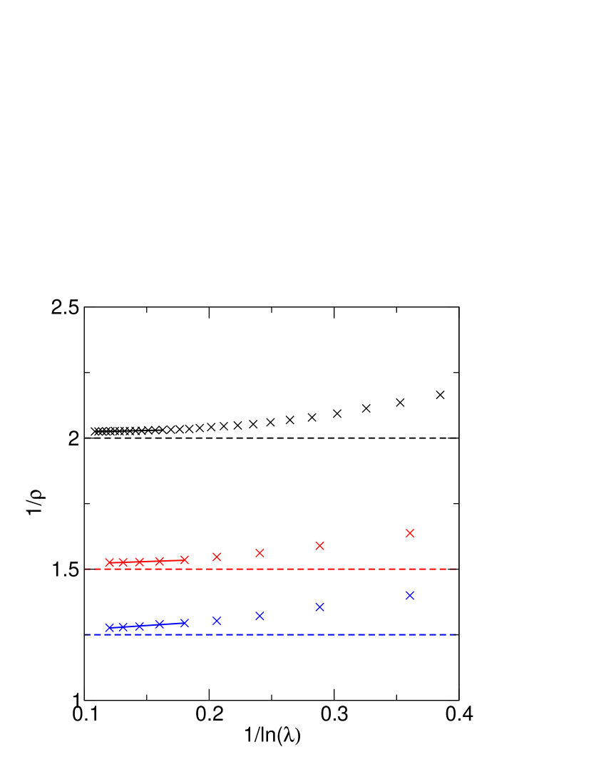
Figure 1: Simulated adsorption Isotherms. $\rho_{s}=1,2,4$ top to bottom. The dashed lines show the predictions of Eq. (10).

III.2 Numerical verification of the suggested mapping

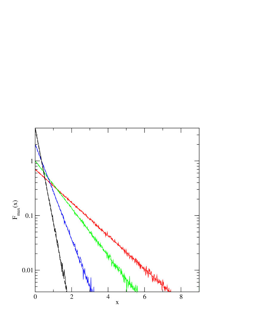
Figure 2: Gap distribution function $F_{\rm max}(x)$ for configurations of hard rods at infinite activity on the random site surface with $\rho_{s}=0.7,1,2.0,4.0$ from right to left, bottom. The dashed lines are the predictions of Eq.(11) The solid lines correspond to the simulation results.

.

We confirmed Eq. (10) in two ways. The first generates configurations of maximum density directly. A number $n_{s}$ points are distributed uniformly and randomly in the unit interval. The first site is occupied by a rod of length $\sigma=1/n_{s}$. Each site to the right is checked in order until one is found that is at least a distance $\sigma$ from the occupied one. This site is occupied and the process iterated until all sites have been accounted for. A number of averages over different configurations of sites is performed. We also verified Eq. (10) by determining the adsorption isotherms for different values of the site density $\rho_{s}$ and taking the limit $\lambda\to\infty$: See Fig. 1.

For the hard rod fluid at equilibrium the gap distribution function is given exactly by:

$$F(\rho,x)=\frac{\rho}{1-\rho}\exp(-\frac{\rho\,x}{1-\rho}).$$ (16)

The gap distribution function calculated for the densest configurations of the random site model is in agreement with the predictions of Eq. (16) using a density computed from Eq. (10), confirming that the configuration of rods on the random site surface has the same structure as the equilibrium hard rod fluid at the same density (see Fig.2). This is consistent with the behavior of a related lattice model for which we showed that there is an exact mapping to the system without disorder at infinite activityTalbot et al. (2007).

In order to use Eq.(12) to estimate the maximum coverage of the RSM in two-dimensions, we combine it with the approximate equation of state for hard disks on a continuous surface, which was proposed by WangWang (2002):

$$\frac{\beta P}{\rho}=1+\frac{D}{1-\theta/\theta_{0}}-(D+2a\theta+4b\theta^{2}+8c\theta^{3}+16d\theta^{4}+32e\theta^{5})$$ (17)

where $\theta=\pi\sigma^{2}\rho/4$ is the coverage, $\theta_{0}=0.907..$ is the coverage of a hexagonal close-packed configuration, $D=4.08768,a=1.25366,b=0.46051,c=0.152797,d=0.04412,e=0.00929.$. For a given value of the site density, $\rho_{s}$, Eq. (17) is solved numerically for $\theta$. It is convenient to introduce the dimensionless site density

$$\alpha=\frac{\pi}{4}\sigma^{2}\rho_{s}$$ (18)

The results, shown in Fig. 3 are in excellent agreement with the simulation results for the entire range of $\alpha$. This should be compared with cluster expansion to second order that gives good predictions only for $\alpha\lesssim 0.3$Oleyar and Talbot (2007). Note that the approximate equation of state, Eq.(17), does not include the possible presence of a phase transition.

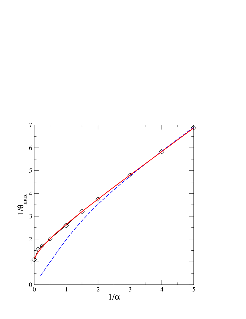
Figure 3: Maximum coverage of the RSM as a function of the dimensionless site density. The symbols show the simulation results, the dashed line is the cluster approximation to second order Oleyar and Talbot (2007), and the solid line shows the predictions of Eqs. (12) and (17).

.

Figure 4: Lowest order clusters of adsorption sites. A solid line connects two sites that are closer than $\sigma$ and a dashed line indicates that two sites are further apart than $\sigma$. Triplets of type “3a” (left) and “3b” (right) are shown left to right in the second row. The expression to the right of the clusters is the corresponding grand canonical partition function for the adsorbed particles.

IV RSM in one dimension

IV.1 Low site density expansion

To provide a description of the adsorption isotherms at finite activity, it is useful to consider an expansion in the density of adsorption sites. Assuming that the adsorption surface consists of isolated clusters of sites, the (averaged) logarithm of the partition function may be expressed as

$$\overline{\ln\Xi}=N_{1}\ln\Xi_{1}+N_{2}\ln\Xi_{2}+N_{3a}\ln\Xi_{a}+N_{3b}\ln\Xi_{3b}+...,$$ (19)

where $N_{i}=x_{i}N_{s}$ is the number of clusters of type $i$ and $i\equiv(n,a)$ with $n$ being the number of sites in the cluster and $a$ characterizing when necessary the subclass of clusters (see Fig.4). This simple expansion is possible because adsorption on a given cluster does not affect any of the others. The adsorption isotherm is then

$$\rho A=\lambda N_{1}\left(\frac{\partial\ln\Xi_{1}}{\partial\lambda}\right)+\lambda N_{2}\left(\frac{\partial\ln\Xi_{2}}{\partial\lambda}\right)+...,$$ (20)

which gives

$$\rho =\lambda\rho_{s}\bigl{(}x_{1}\frac{1}{1+\lambda}+\frac{2}{1+2\lambda}x_{2}$$

$$+ \frac{3+2\lambda}{1+3\lambda+\lambda^{2}}x_{3a}+\frac{3}{1+3\lambda}x_{3b}+...\bigr{)}.$$ (21)

In one-dimension, exact expressions can be obtained for the first few clusters following the approach of Quintanilla and Torquato Quintanilla and Torquato (1996):

$$x_{1} =\exp(-2\rho_{s})$$ (22)

$$x_{2} =\exp(-2\rho_{s})(1-\exp(-\rho_{s}))$$ (23)

$$x_{3a} =\exp(-3\rho_{s})(\exp(-\rho_{s})+\rho_{s}-1)$$ (24)

$$x_{3b} =\exp(-2\rho_{s})(1-(1+\rho_{s})\exp(-\rho_{s}))$$ (25)

where $x_{2}$, for example, is the number of clusters with two linked sites (per adsorption site). At the triplet level we need to distinguish between two subclasses of clusters shown in Fig. 4. In type “3a” two of the sites can be simultaneously occupied, while in type “3b” only one of the sites can be occupied since all are mutually closer than the particle diameter.

The predictions of Eq. (IV.1) are compared with the simulation results in Fig. 5. The expansion to third order provides a good description of the isotherm for $\rho_{s}=0.2$, but the quality deteriorates rapidly for larger site density. Eq. (IV.1) is unable to predict the correct limit when $\lambda\rightarrow\infty$. This disagreement is more pronounced when $\rho_{s}$ increases: for instance, when $\rho_{s}=1$, the expansion fails completely, because the predicted density is lower than for $\rho_{s}=0.5$.

Since the above expansion is limited to small values of $\rho_{s}$, we simplify Eq. (IV.1) by performing a series expansion in $\rho_{s}$, giving

$$\rho =\lambda\rho_{s}\bigl{(}\frac{1}{1+\lambda}-\frac{2\lambda}{(1+\lambda)(1+2\lambda)}\rho_{s}$$

$$+ \frac{\lambda^{2}(12\lambda^{2}+29\lambda+9)}{2(1+\lambda)(1+2\lambda)(1+3\lambda)(1+3\lambda+\lambda^{2})}\rho_{s}^{2}+O(\rho_{s}^{3})\bigr{)}$$ (26)

We note that Eq. (IV.1) can be expressed as

$$\rho(\rho_{s},\lambda) =\sum_{l=1}^{3}\left(-\left(\frac{-\lambda}{1+\lambda}\right)^{l}+F_{l}(\rho_{s},\lambda)\right)\rho_{s}^{l}$$ (27)

where $F_{l}(\rho_{s},\lambda)$ represents the remaining terms in the exact expansion and, consistent with these terms, has the property that $F_{l}(\rho_{s},\lambda)\to 0$ when $\lambda\to 0$ and $\lambda\to\infty$. This property has been verified order by order for a random lattice modelTalbot et al. (2007), and only for the three first orders for this model. If we partially resum the series, neglecting the remaining terms, we obtain that

$$\rho(\rho_{s},\lambda) =\frac{\lambda\rho_{s}}{1+\lambda(1+\rho_{s})}$$ (28)

Although the site density expansion, Eq. (IV.1), is valid only for small $\rho_{s}$, the partial resummation leads to an expression for $\rho$ that is exact in the limit of very large activities $\lambda$, whatever the value of $\rho_{s}$. It thus provides a sensible approximation based on the site density expansion.

Isotherms given by Eq. (28) are plotted in Fig. 5 (dotted curves). Although for very low site density the third order expansion gives a better estimation, the quality of Eq. (28) is significantly better for $\rho_{s}=0.5$, and it always gives the saturation density exactly. For larger values of the site density, $\rho_{s}>1$, the approximation overestimates the adsorbed amount for intermediate activities. This is expected since the neglected terms are non-zero for intermediate bulk activity. Attempts to obtain a better resummation of the series expansion, Eq. (IV.1), were fruitless. Therefore, we follow the approach that we used in our study of the model of dimer adsorptionTalbot et al. (2007), by introducing an effective activity.

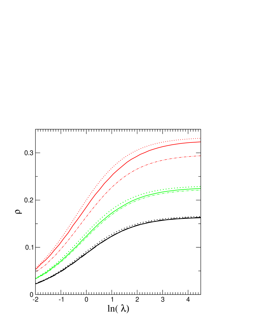
Figure 5: Adsorption isotherms versus activity $\lambda$ for several site densities: $\rho_{s}=0.5,0.3,0.2$ from top to bottom. The dash-dotted and dotted lines show the predictions of Eq. IV.1 (exact expansion to third order in $\rho_{s}$) and Eq. 28, respectively. The solid lines show the simulation results.

.

IV.2 Effective activity approach

Despite the exact mapping found in the infinite activity limit, no simple reasoning can be used to obtain exact results at finite bulk activity. We therefore investigated several approximate methods, the most successful of which is based on an effective activity.

The equation of state of the hard rod fluid on a continuous line is Tonks (1936)

$$\beta P=\frac{\rho}{1-\rho\sigma}$$ (29)

According to the results in Section III, the hard rod fluid at a pressure $\beta P=\rho_{s}$ has the same density (obtained by inverting Eq. (29)) as the densest configuration of hard spheres on the random site surface, Eq. (10). We seek a generalization of this mapping for an arbitrary value of the bulk phase activity, i.e. an effective activity $\lambda_{\rm eff}$ such that the density of adsorbed rods in the RSM, $\rho(\rho_{s},\lambda)$ is given by

$$\rho(\rho_{s},\lambda)=\rho^{*}(\lambda_{\rm eff}(\lambda,\rho_{s})),$$ (30)

where $\rho^{*}(\lambda)$ is the density of rods on a continuous substrate at an activity $\lambda$. This is given exactly by

$$\rho^{*}(\lambda)=\frac{L_{w}(\lambda)}{1+L_{w}(\lambda)},$$ (31)

where $L_{w}(x)$, the Lambert-W function, is the solution of $x=L_{w}(x)\exp(L_{w}(x))$. The inverse relation is

$$\lambda=\frac{\rho}{1-\rho}\exp\bigl{(}\frac{\rho}{1-\rho}\bigr{)}.$$ (32)

From the exact result, Eq. (10), we have that $\lambda_{\rm eff}(\lambda=\infty)=\rho_{s}e^{\rho_{s}}$. Taking Eqs. (31) as a mere definition of $\lambda_{\rm eff}(\lambda,\rho_{s})$, we have computed it from the simulated adsorption isotherms. Results are shown in Figs. 6-8 and will be used as a reference for testing the validity of various approximations.

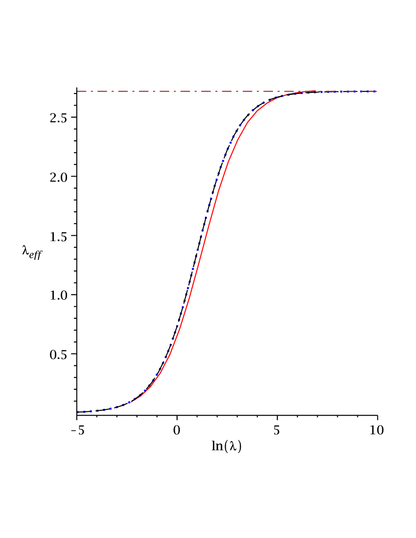
Figure 6: Effective activity $\lambda_{\rm eff}$ as a function of the logarithm of the activity $\ln\lambda$ with $\rho_{s}=1$. The solid line shows the simulation result, calculated from the density by using Eq. (32). The predictions of Eq. (33) combined with Eq. (34) and Eq.(36) are shown as dotted and dashed lines, respectively. They are almost indistinguishable. The horizontal dashed line shows the exact limiting value of $\rho_{s}e^{\rho_{s}}$.

.

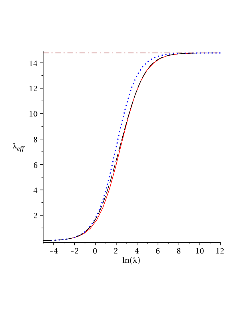
Figure 7: Same as Fig. 6, except that $\rho_{s}=2$. The prediction of Eq. (36) is now more accurate than that of Eq. (34).

.

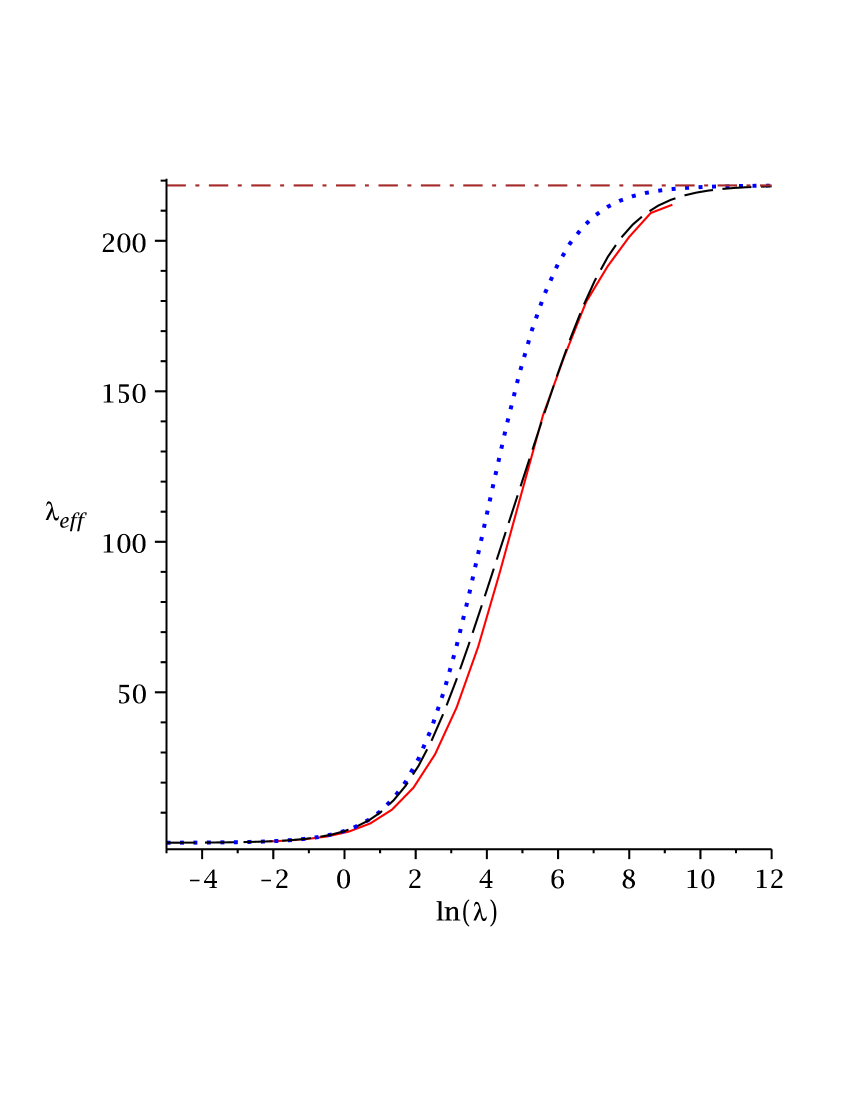
Figure 8: Same as Fig. 7, except that $\rho_{s}=4$. Eq. (34) fails to reproduce the simulation data for intermediate value of $\ln(\lambda)$ whereas the prediction of Eq. (36) remains accurate.

.

Following the method introduced in the study of the lattice modelTalbot et al. (2007), we attempt to construct simple expressions that can reproduce the numerical results, when available and describe the isotherms for a wide range of parameters $\rho_{s}$ and $\lambda$. The effective activity as a function of the activity $\lambda$ and of the density site $\rho_{s}$ can be written as

$$\frac{1}{\lambda_{\rm eff}}=\frac{f(\rho_{s},\lambda)}{\rho_{s}\lambda}+\frac{1}{\rho_{s}e^{\rho_{s}}}$$ (33)

where $f(\rho_{s},\lambda)$ is a function to be determined. We know that at small $\lambda$, the exact behavior is given by $\lambda_{\rm eff}=\rho_{s}\lambda$, which imposes that $f(\rho_{s},\lambda)$ goes to $1$. Conversely, when $\lambda$ is large, the effective activity $\lambda_{\rm eff}$ behaves as $\rho_{s}e^{\rho_{s}}+O(\lambda)$, which leads to the constraint that $\lim_{\lambda\rightarrow\infty}f(\rho_{s},\lambda)=A(\rho_{s})$ where $A(\rho_{s})$ is an unknown function of $\rho_{s}$. If $A(\rho_{s})$ remains close to one, the simplest choice consists of choosing

$$f(\rho_{s},\lambda)=1$$ (34)

for all values of $\lambda$. While this simple choice gives a fair agreement with the simulated values when $\rho_{s}=1$ (see Fig. 6), the situation deteriorates for larger values of $\rho_{s}$ (see Figs. 7- 8). However, contrary to the one-dimensional lattice model, we do not know the exact asymptotic behavior of $f(\rho_{s},\lambda)$ for large $\lambda$. In order to improve the description, we consider a homographic function of $\lambda$ verifying the exact behavior, when $\lambda\rightarrow 0$ and $\lambda\rightarrow\infty$,

$$f(\rho_{s},\lambda)=\frac{A(\rho_{s})\lambda+B(\rho_{s})}{\lambda+B(\rho_{s}),}$$ (35)

where $A(\rho_{s})$ and $B(\rho_{s})$ are unknown functions. Examination of the series expansion in the limit of infinite bulk activity suggests that $B(\rho_{s})$ should grow as $e^{\rho_{s}}$ in order to give the right behavior. In the absence of additional criteria, we have chosen $A(\rho_{s})=\rho_{s}$ and $B(\rho_{s})=\rho_{s}e^{\rho_{s}}$, which gives

$$f(\rho_{s},\lambda)=\frac{\rho_{s}(e^{\rho_{s}}+\lambda)}{\lambda+\rho_{s}e^{\rho_{s}}}.$$ (36)

Note that when $\rho_{s}=1$, this function gives $f(\rho_{s},\lambda)=1$. Figs. 6- 8 show that the quality of the approximation given by Eq. (33) and Eq. (34) deteriorates with increasing $\rho_{s}$. This is a consequence of the fact that the asymptotic approach to the saturated state is not correctly captured with this simple approximation. A better agreement with simulations is obtained by using Eq.(33) and Eq.(36) for $\rho_{s}=2$ and $\rho_{s}=4$ (see Figs. 7 and 8).

The purpose of this exercise is ultimately to obtain an approximate, but accurate, description of the adsorption isotherms. This is done by substituting Eq. (33) in Eq. (31). Fig. 9 shows a comparison of these estimates with the simulation results. The effective activity approach is a considerable improvement over the cluster expansion, whose accuracy is restricted to small density site $\rho_{s}<0.5$ (c.f. Fig. 5) and allows one to describe adsorption even when $\rho_{s}>1$.

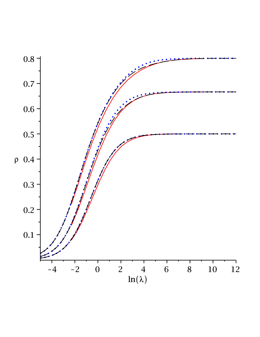
Figure 9: Adsorption isotherms versus activity $\lambda$ for several site densities: $\rho_{s}=1,2,4$, predicted by the effective activity approach, Eqs. (32) and (31) by using Eq. (34) (dotted lines) and combined with Eq. (36) (dashed lines). The solid lines show the simulation results.

.

IV.3 Structure

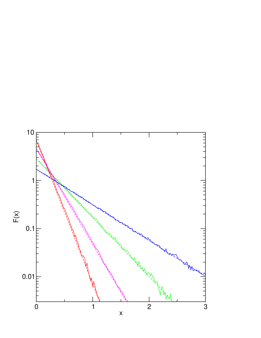
Figure 10: Gap distribution function for configurations of hard rods at finite activity on the random site surface with $\rho_{s}=10$. The dashed lines are the predictions of Eq. 16 with a density given by the equilibrium isotherm value and the solid lines show the simulation results. $\lambda=1,5,50,1000$ from left to right in the bottom part.

.

We have also examined the structure of the hard-rod configurations at finite activity. As in the case of the lattice modelTalbot et al. (2007), we do not expect an exact mapping to the homogeneous system at the same density. Nevertheless, as shown in Fig. 10, the distributions computed from the simulation are very well described by Eq. (16) with a density equal to the equilibrium isotherm value.

V Two-dimensional model

We construct approximate isotherms in the same way as for one-dimensional model, i.e. by introducing an effective activity as a function of bulk activity.

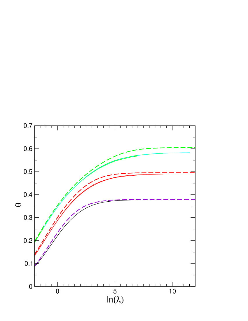
Figure 11: Adsorption Isotherms for dimensionless site densities $\alpha=1,2,4$ from bottom to top. The dashed lines show the predictions of Eq.(V) combined with Eq.(40). The solid lines show the simulation results obtained with 20 realizations of $n_{s}=2000$ sites.

.

We first consider the homogeneous hard-disk system. We determine the Helmholtz free energy per particle by integration along the isotherms:

$$\beta f^{ex}=\int_{0}^{\theta}\left(\frac{\beta P}{\rho}-1\right)\frac{d\theta^{\prime}}{\theta^{\prime}}.$$ (37)

The excess chemical potential can then be obtained from

$$\beta\mu^{ex}=\beta f^{ex}+\theta\frac{\partial\beta f^{ex}}{\partial\theta}.$$ (38)

By inserting the approximate equation of state, Eq. (17) in Eq.(37), and substituting the result in Eq. (38), one obtains for the activity, $\lambda=\exp(\beta\mu)$ the relation

$$\ln(\lambda)=\ln(4\theta/\pi)-{\frac{96}{5}}\,e{\theta}^{5}-20\,d{\theta}^{4}-{\frac{32}{3}}\,c{\theta}^{3}-6\,b{\theta}^{2}-4\,a\theta$$

$$-D\ln\left(1-\frac{2\,\sqrt{3}}{\pi}\theta\right)+2\,{\frac{D\sqrt{3}\theta}{\pi-2\,\sqrt{3}\theta}},$$ (39)

where, we recall, $\theta=\pi\sigma^{2}\rho/4$.

The isotherm for the $2D$ RSM can be calculated by following a procedure similar to that used in the one-dimensional case. By means of Eq. (12), one obtains the saturation coverage when the bulk activity is infinite, $\theta_{\infty}$. Then, by inserting this quantity in Eq. (V), the effective activity $\lambda_{\rm eff}^{\infty}\equiv\lambda_{\rm eff}(\theta_{\infty})$ is obtained.

The counterpart of Eq. (33) for the two-dimensional system is now

$$\frac{1}{\lambda_{\rm eff}}=\frac{1}{\rho_{s}\lambda}+\frac{1}{\lambda_{\rm eff}^{\infty}}$$ (40)

where, in the absence of more information, we have set $f(\rho_{s},\lambda)=1$.

Therefore, at a given bulk activity $\lambda$ and site density $\rho_{s}$, one obtains an effective activity by using Eq. (40), and by inserting the effective activity in Eq. (V), one deduces the corresponding coverage in the 2D RSM.

Fig. 11 compares the simulation results and the approximate isotherms for different values of the site density. While the agreement is not perfect, the scheme represents a major improvement compared to the pertubative approach (third-order density expansion) for describing situations where the density site is moderate to high and allows one to develop new approximate isotherm equations.

VI Conclusion

We have presented a theoretical and numerical study of the reversible adsorption of hard spheres on randomly distributed adsorption sites. Unlike the case of irreversible adsorption, there is no simple mapping between the RSM and a system of hard spheres on a homogeneous surface. We have, nonetheless, been able to obtain some exact results in various limits: small and large bulk activity and small and large site density. We have proposed an effective activity approach, which interpolates between the known behavior, to obtain an approximate description for intermediate situations. The adsorption isotherms predicted by this approach are in excellent agreement with simulation results. In the two-dimensional case, we have not investigated phase transitions in detail, although there does appear to be a solid-like phase for sufficiently high site density and activity. It will also be interesting to investigate reversible adsorption on a substrate when a second source of disorder is present: distribution of adsorption site energies. The present approach should apply to this case as well.

Appendix A Random Site Model: beyond the continuum limit

The sites being uncorrelated, Eq.(4), one easily obtains the connected $n$-site correlated functions $\left(\overline{\eta({\bf r}_{1})\eta({\bf r}_{2})...\eta({\bf r}_{n})}\right)_{c}$ which read

$$\left(\overline{\eta({\bf r}_{1})\eta({\bf r}_{2})...\eta({\bf r}_{n})}\right)_{c}=\rho_{s}\prod_{i<j}\delta({\bf r}_{i}-{\bf r}_{j}).$$ (41)

The $n$-site correlation functions which appear in Eq.(1) can be obtained from the above connected functions by using an expansion in the (mean) site density:

$$\overline{\eta({\bf r}_{1})\eta({\bf r}_{2})...\eta({\bf r}_{n})}=\rho_{s}^{n}+\rho_{s}^{n-2}\sum_{i<j}\left(\overline{\eta({\bf r}_{i})\eta({\bf r}_{j})}\right)_{c}$$

$$+\rho_{s}^{n-3}\sum_{i<j<k}\left(\overline{\eta({\bf r}_{i})\eta({\bf r}_{j})\eta({\bf r}_{k})}\right)_{c}$$

$$+\rho_{s}^{n-4}\sum_{i<j<k<l}\left(\overline{\eta({\bf r}_{i})\eta({\bf r}_{j})\eta({\bf r}_{k})\eta({\bf r}_{l}))}\right)_{c}$$

$$+\rho_{s}^{n-4}\sum_{i<j}\left(\overline{\eta({\bf r}_{i})\eta({\bf r}_{j})}\right)_{c}\sum_{i<k<l}\left(\overline{\eta({\bf r}_{k})\eta({\bf r}_{l})}\right)_{c}$$

$$+...$$ (42)

The expression of the higher-order terms rapidly becomes tedious.

On the other hand, the $n$-body connected density functions of a homogeneous hard sphere system at activity $z$ are given by functional derivatives of the the logarithm of grand-canonical function (see Eq.(3))

$$\rho^{(p)*}_{c}({\bf r}_{1}{\bf r}_{2}...{\bf r}_{p}|z)=\left.\frac{\delta^{p}\ln(\Xi^{*}(z({\bf r})))}{\delta z({\bf r}_{1})\delta z({\bf r}_{2})...\delta z({\bf r}_{p})}\right|_{z({\bf r})=z}$$

$$=\sum_{n=p}^{\infty}\frac{z^{n}}{(n-p)!}\int d{\bf r}_{p+1}...d{\bf r}_{n}U_{n}({\bf r}_{1},{\bf r}_{2}...{\bf r}_{p},{\bf r}_{p+1}...{\bf r}_{n}).$$ (43)

By inserting Eq.(A) in Eq.(3) and by using Eq.(A), the disorder averaged logarithm of the partition function of the RSM has the following expansion:

$$\overline{\ln(\Xi)}=\ln(\Xi^{*}(z))+\frac{1}{2\rho_{s}}\int d{\bf r}_{1}\rho_{c}^{(2)*}({\bf r}_{1},{\bf r}_{1}|z)$$

$$+\frac{1}{3!\rho_{s}^{2}}\int d{\bf r}_{1}\rho_{c}^{(3)*}({\bf r}_{1},{\bf r}_{1},{\bf r}_{1}|z)$$

$$+\frac{1}{4!\rho_{s}^{3}}\int d{\bf r}_{1}\rho_{c}^{(4)*}({\bf r}_{1},{\bf r}_{1},{\bf r}_{1},{\bf r}_{1}|z)$$

$$+\frac{1}{4\rho_{s}^{2}}\int d{\bf r}_{1}d{\bf r}_{2}\rho_{c}^{*(4)}({\bf r}_{1},{\bf r}_{1},{\bf r}_{2},{\bf r}_{2}|z)$$

$$+...$$ (44)

For hard spheres, the non-overlapping property leads to a simple expression for the n-body connected density function

$$\rho_{c}^{(p)*}({\bf r}_{1},{\bf r}_{1},..,{\bf r}_{1},{\bf r}_{1}|z)=(-1)^{p-1}(p-1)!\rho^{*}(z)^{p}.$$ (45)

A straightforward but more tedious calculation allows one to obtain

$$\rho_{c}^{(4)*}({\bf r}_{1},{\bf r}_{1},{\bf r}_{2},{\bf r}_{2}|z)=4\rho^{*}(z)^{2}\rho_{c}^{(2)*}({\bf r}_{1},{\bf r}_{2})-2\rho_{c}^{(2)*}({\bf r}_{1},{\bf r}_{2})^{2}$$ (46)

By inserting Eqs.(45) and (46) in Eq.(A), one obtains that

$$\frac{\overline{\ln(\Xi)}}{A}=\frac{\ln(\Xi^{*}(z))}{A}+\left(-\frac{\rho^{*}(z)^{2}}{2\rho_{s}}+\frac{\rho^{*}(z)^{3}}{3\rho_{s}^{2}}-\frac{\rho^{*}(z)^{4}}{4\rho_{s}^{3}}\right)$$

$$+ \frac{\rho^{*}(z)^{4}}{2\rho_{s}^{2}}\int d{\bf r}(2h^{*}({r}|z)-(h^{*}({r}|z)))^{2}$$ (47)

where $h^{*}(r|z)$ is the radial pair correlation correlation of the hard-sphere model at the activity $z$Hansen and McDonald (1976). It is worth mentioning that the second term of the rhs of Eq.(A) corresponds to successive terms of a series expansion that can be resummed, and finally, one obtains that

$$\frac{\overline{\ln(\Xi)}}{A}=\frac{\ln(\Xi^{*}(z))}{A}+\rho_{s}\ln\left(1+\frac{\rho^{*}(z)}{\rho_{s}}\right)-\rho^{*}(z)$$

$$+ \frac{\rho^{*}(z)^{4}}{2\rho_{s}^{2}}\int d{\bf r}(2h^{*}({r}|z)-(h^{*}({r}|z))^{2})+O(1/\rho_{s}^{3}).$$ (48)

References

- Bakaev (2004) V. A. Bakaev, Surface Science 564, 108 (2004).
- Adamczyk et al. (2002) Z. Adamczyk, B. Siwek, P. Weronski, and E. Musial, Applied Surface Science 196, 250 (2002).
- Dabrowski (2001) A. Dabrowski, Adv Colloid Int Sci 93, 135 (2001).
- Adamczyk et al. (2005) Z. Adamczyk, K. Jaszczolt, A. Michna, B. Siwek, L. Szyk-Warszynska, and M. Zembala, Adv Colloid Int Sci 118, 25 (2005), ISSN 0001-8686.
- Jaroniec and Madey (1988) M. Jaroniec and R. Madey, Physical adsorption on heterogeneous solids (Elsevier, 1988).
- W.Rudzinski and Everett (1992) W.Rudzinski and D. H. Everett, Adsorption of Gases on Heterogeneous Surfaces (Academic Press, 1992).
- Johnson et al. (1996) R. D. Johnson, Z. G. Wang, and F. H. Arnold, J. Phys. Chem. 100, 5134 (1996).
- Talbot et al. (2007) J. Talbot, G. Tarjus, and P. Viot, Phys. Rev. E 76, 051106 (2007).
- Oshanin et al. (2003a) G. Oshanin, O. Bénichou, and A. Blumen, J. Stat. Phys. 112, 541 (2003a).
- Oshanin et al. (2003b) G. Oshanin, O. Bénichou, and A. Blumen, Europhys. Lett 62, 69 (2003b).
- Jin et al. (1993) X. Jin, N. H. L. Wang, G. Tarjus, and J. Talbot, J. Phys. Chem. 97, 4256 (1993).
- Oleyar and Talbot (2007) C. Oleyar and J. Talbot, Physica A 376, 27 (2007).
- Ostuni et al. (2003) E. Ostuni, B. A. Gryzbowski, M. Mrksich, C. S. Roberts, and G. M. Whitesides, Langmuir 19, 1861 (2003).
- Lüthgens and Janshoff (2005) E. Lüthgens and A. Janshoff, ChemPhysChem 6, 444 (2005).
- Weight and Hartmann (2000) M. Weight and A. K. Hartmann, Phys. Rev. Lett. 26, 6118 (2000).
- Weight and Hartmann (2001) M. Weight and A. K. Hartmann, Phys. Rev. E 63, 056127 (2001).
- Rosinberg et al. (1994) M. L. Rosinberg, G. Stell, and G. Tarjus, J. Chem. Phys. 100, 5172 (1994).
- Hansen and McDonald (1976) J.-P. Hansen and I. R. McDonald, Theory of Simple Liquids (Academic Press, 1976).
- Stell (1976) G. Stell, Phase transitions and critical phenomena (Academic Press, 1976), p. 205.
- Tonks (1936) L. Tonks, Phys. Rev. E 50, 955 (1936).
- Torquato (1995) S. Torquato, Phys. Rev. E 51, 3170 (1995).
- Rintoul et al. (1996) M. D. Rintoul, S. Torquato, and G. Tarjus, Phys. Rev. E 53, 450 (1996).
- Viot et al. (1998) P. Viot, P. R. V. Tassel, and J. Talbot, Phys. Rev. E 57, 1661 (1998).
- Wang (2002) X. Z. Wang, Phys. Rev. E 66, 031203 (2002).
- Quintanilla and Torquato (1996) J. Quintanilla and S. Torquato, Phys. Rev. E 54, 5331 (1996).