Topological structures in the equities market network

Abstract.

We present a new method for articulating scale-dependent topological descriptions of the network structure inherent in many complex systems. The technique is based on “Partition Decoupled Null Models,” a new class of null models that incorporate the interaction of clustered partitions into a random model and generalize the Gaussian ensemble. As an application we analyze a correlation matrix derived from four years of close prices of equities in the NYSE and NASDAQ. In this example we expose (1) a natural structure composed of two interacting partitions of the market that both agrees with and generalizes standard notions of scale (eg., sector and industry) and (2) structure in the first partition that is a topological manifestation of a well-known pattern of capital flow called “sector rotation.” Our approach gives rise to a natural form of multiresolution analysis of the underlying time series that naturally decomposes the basic data in terms of the effects of the different scales at which it clusters. The equities market is a prototypical complex system and we expect that our approach will be of use in understanding a broad class of complex systems in which correlation structures are resident.

1. Introduction

Complex systems often arise as a consequence of multilayered interactions among a large population of diverse agents. For example, neural capabilities arise as a result of the interactions of clusters of neurons of similar function [1]. Social networks often function as interacting hierarchies of sub-networks [2, 3], as do link networks for webpages [4]. The dynamics of the equities market is driven by interactions among sectors, which are in turn influenced by their component industries as well as by the strategies of large institutional traders [5]. The financial markets are of particular interest for researchers in complex systems, as their intrinsically numerical nature provides a wealth of data for analysis and hypothesis testing. The significant complexity of the web of interdependence in the markets has a natural and informative mathematical formulation in terms of a network encoding the correlation structure of some underlying time series (e.g., price and volume) that measures something of the state of the financial instrument. Indeed, such correlation networks are an important class of networks that fall naturally into the larger class of complex phenomena in which entities are related according to some measure of similarity in a complex system.

In this paper we present a new tool for decomposing these kinds of correlation networks — the “Partition Decoupling Method.” It is an iterative method in which spectral considerations (i.e., eigenvalues of a relevant matrix) are used to identify significant clusters via comparison to some relevant random model. The effect of these clusters is removed from the underlying data to reveal a residual layer of interaction ready for another round of structural decomposition. In this way, the correlation network, as a summary of some complex system, provides the nexus for an interesting symbiosis between the ideas of multiscale data analysis and topological network analysis. The iterated removal of the “cluster effect” is akin (in spirit) to the well-known “multiresolution analysis” that accompanies wavelet decompositions in signal and image processing (see e.g., [7, 8], as well as [9] which contains a more general view of multiresolution analysis). It is likewise similar to a factor or principal component analysis [10] that creates a succession of approximations to a correlation matrix.

Our approach produces a sequence of partitions of the network, each providing a topological description of an aspect of the network structure. This in turn gives rise to natural hierarchical decompositions of the underlying data stream. The hierarchical structure of the data is also manifested in a multiscale structure in the correlation. The derived partitions suggest a new class of null models introduced herein, the Partition Decoupled Null Model (PDNM), which incorporates the different clusters into a random model. A PDNM is best understood as a generalization of the widely used Gaussian ensemble (GE) null model in which there is a natural incorporation of the structural information associated with the partitions. The PDNM carries with it several interacting partitions, each with its own geometric structure, making it a more textured and potentially more powerful model for comparison. We anticipate that the Partition Decoupling Method (PDM) will be of use in a variety of disciplines in which structure based on similarity measures (e.g., correlation) is expected.

As an example, we give a multipartition analysis of the correlation network of a portion of the equities market. A multiresolution, multipartition decomposition of the equities market is plausible as the global structure of these dynamic entities is emergent from huge numbers of local interactions resulting from several different factors reflecting the dynamics of supply and demand on various scales.

Within each partition, we expose a multiscale network in which nodes at any given scale are aggregations of nodes at a finer scale. The nodes both echo and extend the usual notion of sector in the market. The articulation of topological structure yields our second main result — the unsupervised discovery of non-trivial homology (loops) in the network of clusters, reflecting the well-known phenomenon of capital movement called “sector rotation.”

Ultimately, we reveal that the equities market is best described as a collection of processes defined on interacting networks — a characterization shared by many diverse complex systems. We demonstrate that by a careful decoupling of network partitions, we may peel apart the layers of network structure to reveal subtle interdependencies among network components as well as residual network structures hitherto masked by more dominant network processes.

Our approach differs in some important ways from previous applications of clustering techniques to the hierarchical decomposition of complex systems — and particularly from previous efforts in the articulation of “market topology” as manifested in correlation networks derived from equities. The most important difference is that our model is not strictly hierarchical, but instead details the interaction between a number of different partitions of the network. Our method places no constraint on connectivity of the nodes, whereas purely hierarchical approaches constrain the complexity (in terms of connectivity) of the defined nodes in some manner (e.g., as a tree [11] or with some fixed bound on topological type [12]). Furthermore, while our use of the GE null model (see the Methodology section) as a means of identifying relevant information in our clustering step is in the spirit of random matrix null models [13, 14, 15], our method provides a more detailed description of a network by identifying relevant clusters across multiple interacting partitions. We also note that, in contrast to our clustering method, cluster identification using localization of eigenvectors (e.g. [13]) generally produces clusters which do not necessarily partition the entire set of equities (however, see [16] for a single partition result).

2. Methodology

There is a natural tension in the analysis of complex systems between the desire to recognize the complexity of a system in its entirety and the desire to conceptualize the system processes in terms of the interaction of a minimal collection of discrete components. Our methodology is designed to preserve important aspects of system complexity typically lost in the application of dimension reduction techniques. The Partition Decoupling Method is a principled method for generating multipartition descriptions of the system which effectively capture both the dominant structures defining the system as well as second order structures which are often obscured by the actions of the dominant processes. It involves combining two algorithms: the Partition Scrubbing Method and the Hierarchical Spectral Clustering Method.

2.1. Partition Scrubbing Method

Beginning with a discrete sample space of nodes or entities indexed by $I=\{1,\ldots,N\}$ with associated time series $D=\{D(1),\ldots,D(N)\}$ each of length $T$, we identify a collection of characteristic time series $\mathcal{V}$ which capture some aspect of the structure of the $D$ series. Note that these need not be (and rarely are) independent. The idea is that each member of $\mathcal{V}$ summarizes some property of the time series in $D$ and projection of $D$ onto the subspace spanned by $\mathcal{V}$ yields a dimension reduced representation of $D$. From this we then derive a decomposition of $D$ into two orthogonal components– the projection of $D$ onto $\mathcal{V}$ and a residual component $\mathcal{R}$. The process may then be repeated on $\mathcal{R}$, finding a new set of characteristic time series, projecting and computing a second residual component. Iteration may be continued until “failure,” of which there are two types. “Partitioning Failure” occurs when the correlation structure of the residual time series is indistinguishable from the Gaussian ensemble (note that depending on context, this could be replaced by other null models) and we cannot reliably find characteristic times series. “Projection Failure” occurs when the characteristic time series are numerically linearly dependent. In this case the projection on $\mathcal{V}$ does not have a unique representation in terms of the characteristic time series. Our view is that in each iteration, the removal of the effect of the characteristic time series reveals residual structure that may have been masked by the dominant behaviour.

To apply the Partition Scrubbing Method, we start with a collection of normalized sequences $D^{0}(i)$, and a choice of clustering methods for each $0\leq\alpha\leq m$ that, given a collection $D^{\alpha}(i)$, will produce a mapping $C^{\alpha}:I\rightarrow\{1,\dots,|C^{\alpha}|\}$ where $|C^{\alpha}|$ denotes the number of clusters generated by the method (hence $C^{\alpha}$ is assumed to be onto). We calculate the set of characteristic time series associated with the partition:

$$\mathcal{V}^{\alpha}_{k}=mean\{D^{\alpha}(i)|C^{\alpha}(i)=k\}$$

for $1\leq k\leq|C^{\alpha}|$. Then, $\mathcal{V}^{\alpha}=\{\mathcal{V}^{\alpha}_{1},\dots,\mathcal{V}^{\alpha}_{|C^{\alpha}|}\}$.

Next, we scrub the partition to produce $D^{\alpha+1}(i)$ from $D^{\alpha}(i)$. To do so, we decompose $D^{\alpha}(i)$ into the sum of two components: the projection $\mathcal{F}^{{\alpha}}(i)$ associated with the clustering ${\mathcal{C}}^{\alpha}$ and a residual component $\mathcal{R}^{{\alpha}}(i)$, so that:

(1) $$D^{\alpha}=\mathcal{F}^{\alpha}+\mathcal{R}^{\alpha}$$

where

(2) $$\mathcal{F}^{\alpha}(i)=\Pi_{\mathcal{V^{\alpha}}}\left(D^{\alpha}(i)\right)=\sum_{k=1}^{{|C^{\alpha}|}}\tau_{k}^{\alpha}(i)\mathcal{V}_{k}^{\alpha}$$

where $\Pi_{\mathcal{V^{\alpha}}}$ is the projection onto $\mathcal{V}^{\alpha}$.

We assume that $\mathcal{R}^{\alpha}$– the residual component of the time series– is independent of $\mathcal{V}^{\alpha}$. Under these assumptions we can solve for the $\tau_{k}^{\alpha}(i)$ via some simple linear algebra. We call $\tau_{k}^{\alpha}(i)$ the “cluster pressure on node $i$” (at iteration $\alpha$) .

Given these values of $\tau$ we create a new collection of “cleaned” time series:

$$D^{\alpha+1}=norm(\mathcal{R}^{\alpha})=norm(D^{\alpha}-\mathcal{F}^{\alpha})$$

with $norm(\mathcal{R}^{\alpha})=\frac{\mathcal{R}^{\alpha}-m^{\alpha}}{\sigma^{\alpha}}$, where $m^{\alpha}$ and $\sigma^{\alpha}$ denote the mean and standard deviation of $\mathcal{R}^{\alpha}$ respectively.

Using this algorithm, each series $D^{0}(i)$ can be reconstructed from the $D^{m+1}(i)$ from the $\sum_{\alpha=0}^{m}|C^{\alpha}|$ characteristic time series in $\{\mathcal{V}^{\alpha}\}_{\alpha=0}^{m}$ and the $\sum_{\alpha=0}^{m}|C^{\alpha}|+2(m+1)$ parameters $\{m^{\alpha}(i),\sigma^{\alpha}(i),\{\tau^{\alpha}_{k}(i)\}_{k=1}^{|C^{\alpha}|}\}_{\alpha=0}^{m}$ corresponding to the entity. This is our “multiresolution” representation of the original time series data.

2.2. Hierarchical Spectral Clustering Method

To find the partitions needed in the Partition Scrubbing Method, we use an innovative hybrid technique, the Heirarchical Spectral Clustering Method. This method is a principled hierarchical clustering of the correlation network, which proceeds by comparing the eigenvalues of the Laplacian of the correlation network to the eigenvalues of a GE Null Model associated with the network nodes. The method is suitable for networks in which effects of interest tend to result in stratification of network correlation strengths at particular scales. Given a collection of time series indexed by $I$, the output of this method is $n$ levels of clusters of the nodes, each of which provides a partition of $I$.

At the core of the method is the dimension reduction via spectral clustering of the graph Laplacian [17] associated with the correlation matrix. (see the Supplemental Information for an overview of the method). When presented with a correlation matrix for a sequence of time series, we identify the number of significant clusters and perform spectral clustering. To pick the number of significant clusters, we are guided by the use of the GE null model as a means of determining at what point in the spectrum of the Laplacian we are witnessing a manifestation of random effects. $GE(n,m)$ models $n$ nodes with time series of length $m$, drawn from i.i.d. Gaussian random variables. The choice of Gaussian random variables (as opposed to a different distribution) is motivated by our choice of application: the total distribution from the observed data for the equities network is close to Gaussian, with the obligatory fat tails. We set the number of significant clusters equal to the number of nonzero eigenvalues of our correlation matrix which fall below the minimum of the nonzero eigenvalues of the Laplacian of the correlation matrix associated with $GE(n,m)$ after simulating the distribution 100 times.

We call this first set of clusters the first level. To form the remaining levels, we repeat the following two steps until we reach a level with fewer than 2 clusters. Given a level $j$,

1. Form a new correlation matrix $Corr(j)$ by computing the correlations between the mean time series of the clusters of the level $j$.

2. Repeat the comparison to the GE null model and spectral clustering described above to find the $(j+1)^{\text{st}}$ level of clusters (i.e. these are clusters of clusters).

This step fails if at level one the comparison to the GE null model yields less than 2 significant eigenvalues. This we refer to as a Partitioning Failure. We call a level nontrivial if there are greater than 1 significant eigenvalues.

2.3. Partition Decoupling Method (PDM)

The PDM consists of the iterative application of the Partition Scrubbing Method using the partitions produced by the Hierarchical Spectral Clustering Method. As a first step, we normalize the series and we set $C^{0}\equiv 1$. This is akin to defining a partition with a single characteristic time series $\mathcal{V}^{0}$ incorporating all nodes. (In our equities example, this corresponds to removing the global market effect by removing the overall daily mean, and is similar to the normalization used in [13].) Then we proceed by using the Hierarchical Spectral Clustering Method to form the partitions needed by the Partition Scrubbing Method. Notice, to run the Hierarchical Spectral Clustering Method requires choosing a level at each iteration, and we express these choices with the Partition Vector $\langle\ell_{1},\dots,\ell_{m}\rangle$. A partition vector uniquely determines the PDM’s output: the characteristic time series $\{\mathcal{V}^{\alpha}_{\langle\ell_{1},\dots,\ell_{m}\rangle}\}_{\alpha=0}^{m}$ and the constants $\{m^{\alpha}_{\langle\ell_{1},\dots,\ell_{m}\rangle}(i),\sigma^{\alpha}_{\langle\ell_{1},\dots,\ell_{m}\rangle}(i),\{\tau^{\alpha}_{k}(i)\}_{k=1}^{|C^{\alpha}|}\}_{\alpha=0}^{m}$ for each entity. Here $C^{\alpha}_{\langle\ell_{1},\dots,\ell_{m}\rangle}$ denotes the partition formed during the $\alpha$ iteration of the PDM.

Notice the PDM implicitly defines a restricted class of models via constraints on the covariance structures associated with the traditional GE null model. We refer to these associated null models as Partition Decoupled Null Models (PDNM). Given a partition vector $\langle\ell_{1},\dots,\ell_{m}\rangle$, we may construct an associated PDNM by replacing the final $D^{m+1}$ with independent Gaussian random variables and inverting the Partition Scrubbing Method. Notice, if the decomposition terminates with a Partitioning Failure at the $\alpha$ iteration, then the $D^{\alpha+1}$ time series have a correlation structure that is indistinguishable (in the above spectral sense) from the Gaussian ensemble, and this model duplicates the correlation network structure up to random effects. (For decompositions that halt due to a Projection Failure, the residual may still have significant structure when compared to a GE null model, but we cannot reliably compute the contributions of the clusters (i.e. the $\tau_{k}^{\alpha}(i)$)).

This said, we view the importance of the PDM not as providing a complete model of the system, but rather as providing a simple description of the complex system when the complexity is due interacting partitions. For example, to capture the complexity of two interacting partitions with $N$ and $M$ parts respectively might require as many as $MN$ characteristic time series using a hierarchical method. Using the PDM, one can potentially reduce this to $M+N$ characteristic time series, providing much better dimension reduction. Of course a real complex system may not be a simple interaction of $m$ partitions, and different choices of partition vectors may produce different dimension reductions and reveal different structures. We view the PDM as a convenient way to produce a family of distinct dimension reductions, encoded in the tree of partition vectors. In statistical learning situations, this family of dimension reductions can prove to be a valuable asset during the model selection process.

3. Decomposition of Equities Networks

For our specific application to the equities market network, we begin with $N$ time series of daily close prices and create an initial collection of series $D^{0}$ which corresponds to the logarithmic return (logarithmic derivative or fractional change) of the closing price series for each equity. That is, given $P_{t}(i),$ the closing price on day $t$ of equity $i$ we approximate the logarithmic derivative of $P_{t}(i)$ by:

$$D^{0}_{t}(i)=\frac{P_{t}(i)-P_{t-1}(i)}{P_{t-1}(i)}.$$

In this section, we describe the results of applying the PDM to the equities network determined by these series. We demonstrate the ability of the PDM to expose network structures which elude typical clustering methodologies. In doing so, our results delineate a more general notion of market sectors than those typically acknowledged by the industry, in that we expose both recognizable “classical sectors” as well as new natural hybrids. Additionally, the coarse scale analysis successfully exposes a non-trivial homological entity (a topological cycle) corresponding to the known phenomenology of capital flow referred to as “sector rotation.”

For this application, we obtained from the Yahoo! Finance historical stock data server daily close prices for 2547 stocks currently listed on the NYSE and NASDAQ for a period spanning 1251 trading days over (roughly) four years (in the time window from March 15, 2002 - Dec 29, 2006). We began by removing any equity with more than 30% missing data in that window, after which we were left with our 2547 equities over 1251 trading days. In addition, we remove all extreme events from the time series (20 % or larger single day moves). This cleaning was performed in part to avoided having to carefully compensate for the stock splits and reverse stock splits in our data. But we feel that this cleaning would be appropriate even if we had cleaned out the splits via other methods. This is because the structure that underlies the market exists in (at least) two regimes — extreme events and “normal” events — articulated as two different network structures [6]. Since the extreme events were very sparse, the time series correlations we used to explore the equities market by their nature are only capable of illuminating the “normal” network.

PDM Applied the the Equity Market

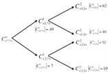
Figure 4. A tree diagram showing the partitions involved when exploring two iteration of the Partition Decoupling Method with respect the equity market example.

To demonstrate the method’s superiority in exposing latent structure in the network, we look at the results of the PDM for two iterations. This resulted in four possible partition vectors with non-trivial levels, as schematically described in figure 4.

We found partitions of the following sizes: $\left|C^{1}_{\langle 1,*\rangle}\right|=49$, $\left|C^{1}_{\langle 2,*\rangle}\right|=7$, $\left|C^{2}_{\langle 1,1\rangle}\right|=62$, $\left|C^{2}_{\langle 1,2\rangle}\right|=10$, $\left|C^{2}_{\langle 2,1\rangle}\right|=52$, and $\left|C^{2}_{\langle 2,2\rangle}\right|=10$. Notice, the partition at the first iteration is independent of future iterations, hence the $*$ can denotes any choice. All of these partition vectors provide effective and distinct dimension reductions of the overall complex system. We now explore these examples with the goal of demonstrating that PDM results in a collection of effective dimension reductions and additionally uncovers information that is often obscured using traditional clustering decompositions.

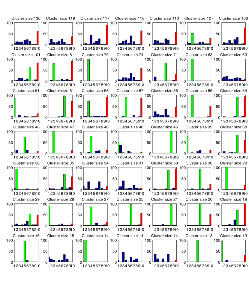
Figure 5. Each figure contains a histogram of the sector and index breakdown of the clusters in $C^{1}_{\langle 1,*\rangle}$. Columns 1-8 represent Yahoo! Finance sector labels. The ninth column is reserved for equities that had no sector labeling. Height of each column is the percentage of the total cluster falling in that category (the cluster size is listed above each histogram). A cluster is defined to be sector dominated if one sector comprises more than 50% of the cluster. In that case, the sector is denoted in green. The tenth column, in red, gives the percentage of the cluster that is listed on the NASDAQ.

For each partition, we use the industry sector labelings available from Yahoo! Finance and NASDAQ/NYSE membership to examine the composition of clusters as both a validation of our clustering method and a tool which helps show when partitions reveal new information. We find that the majority (35 of 49) of the clusters of $C^{2}_{\langle 1,*\rangle}$ are predominantly identified by sector (in the sense that the majority of their nodes are from a given sector) and most of the clusters are strongly identified with either the NASDAQ or the NYSE (see Supplemental Information, Figure 5). Seven of the clusters without dominant sectors have other obvious categorizations (e.g., a regional or business commonality).

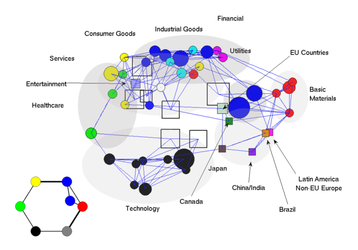
Figure 1. Network structure after after applying PDM and dimension reduction. The big graph is $C^{1}_{\langle 1,*\rangle}$ with distance determined by the correlation between the resulting characteristic time series. Solid circular nodes are classified clusters with coloring indicating the dominant sector or classification. Unfilled square nodes are clusters without a dominant classification labeling. Node size in all cases is proportional to cluster size. Connections (blue lines) are added when the Euclidean distance between two cluster centroids in the Euclidean embedding is in the bottom 10% of all such distances. The grey regions identify clusters of clusters and are (basically) $C^{1}_{\langle 2,*\rangle}$. A schematic drawing of the resulting network is in the lower left hand corner. Nodes are labelled 1-7 counterclockwise beginning with the yellow node.

Clusters of partition $C^{1}_{\langle 2,*\rangle}$ were also classified generally by sector. Figure 1 shows a representation of the network resulting from the spectral clustering algorithm applied in our first iteration. For visualization purposes, we have used the centroids of the clusters in $C^{1}_{\langle 1,*\rangle}$ to represent the entire cluster and have used standard multidimensional scaling (see e.g., [18]) to reduce to a lower dimension. The grey regions in Figure 1 roughly reflect the clusters of $C^{1}_{\langle 2,*\rangle}$. The inset graph in the lower left hand corner shows only the $C^{1}_{\langle 2,*\rangle}$ clusters and is colored according to dominant sector. Tables 2 and 3 provide a precise summary of the clustering data and classification. Clusters of $C^{2}_{\langle 2,1\rangle}$ predominantly admit natural classification (30 out of 52 are classified by sector/industry and 5 more are classified by geography) while the opposite is true of clusters of $C^{2}_{\langle 2,2\rangle}$, where only 3 of 10 admit sector classification (witnessed in Figure 3).

The clusters of $C^{2}_{\langle 2,2\rangle}$ and $C^{2}_{\langle 2,1\rangle}$ provide new partitions of the network and reveal new, textured information previously obscured by behavior of the dominant clusters discovered in the first iteration. While clusters of both $C^{1}_{\langle 1,*\rangle}$ and $C^{2}_{\langle 2,1\rangle}$ are classified by sector and have significant membership overlap, the network configuration is substantially different from that shown in Figure 1. This demonstrates that the clusters of $C^{2}_{\langle 2,1\rangle}$ correspond to a new subsidiary network structure, revealed by exposing new strata of correlation strengths (of lower magnitude) previously masked by the dominant behavior of the clusters in $C^{1}_{\langle 2,1\rangle}$. While the original clustering of the nodes in Technology in $C^{1}_{\langle 2,1\rangle}$ were positively correlated and tightly grouped, the removal of $C^{1}_{\langle 2,1\rangle}$ via partition decoupling exposes a new configuration for these entities in which there is clustering in similar groupings but with different internal relationships, including negative correlations. In Table 1, we see the classification of the clusters into which this technology cluster ($C^{1}_{\langle 2,1\rangle}$) decomposed in $C^{2}_{\langle 2,1\rangle}$. It is evident from this analysis that the partition decoupling has removed the major effect of $C^{1}_{\langle 2,1\rangle}$, revealing lower order effects as expected. We hypothesize that these new partition layers may indicate “second order” trading strategies within these sectors. We note that within the other clusters of $C^{1}_{\langle 2,1\rangle}$, similar effects are found.

The representation of $C^{2}_{\langle 2,2\rangle}$ is shown in Figure 3. The three clusters classified by sector reflect reconfigurations of the sectorial divisions given by $C^{1}_{\langle 2,2\rangle}$. More interesting are the unclassified clusters which reveal new cross-sector interactions. For example, the diamond shaped clusters contain a mixture of multiple sectors. The first is predominantly Consumer Goods, Industrial Goods and Services, while the second is predominantly Financial, Healthcare, Services and Technology. However, both clusters contain significant commonalities. In the first, the equities in the Service sector are almost all related to the shipping industry, which obviously serves to distribute Consumer and Industrial Goods. In the second, the equities in the Financial, Services and Technology sectors are related to companies that either provide services or do business with healthcare companies (e.g. health insurance companies, drug companies, management services, healthcare based REITs, etc.). Equities in both of these clusters are drawn from a range of different clusters in $C^{1}_{\langle 2,2\rangle}$, showing that these two overlapping partitions are truly distinct, and once again demonstrating PDM’s to remove higher order effects and reveal new structure.

Nontrivial homology - sector rotation

The most significant geometric property of the hierarchical network exposed in the first iteration is the existence of a topological cycle (i.e., an example of nontrivial homology) reflective of the well-known phenomenon of sector rotation — which forms the basis for predictive techniques in Intermarket Analysis [19]. Sector rotation refers to the typical pattern of capital flow from sector to sector over the course of a business cycle. Capital flow is echoed in our network structure via enhanced correlations among related equities, and the topological cycle corresponding to sector rotation manifests itself as an emergent structure in the dense network of near neighbor links.

To support the hypothesis that we are exposing sector rotation we compute the effect of the overall market pressure, $\tau$, for each equity in a moving one year window over ten years of data. As most of our clusters are sector dominated, we compute, as a proxy for the aggregate pressure on the clusters, the mean $\tau$ for each sector. In Figure 2, we plot the results over time after applying standard normalization. Both the periodicity of the sector effects and the relative phases of the sector waveforms strongly support the sector rotation interpretation.

The detection of a well-articulated topology in this network is in a similar spirit to that of [20, 21] where the computation of the homology of large datasets is used to topologically classify the data configuration. In our case, the homology has a natural interpretation in terms of observed market behaviour.

4. Conclusion

We present a new method for the decomposition of complex systems given a correlation network structure which yields scale-dependent geometric information — which in turn provides a multiscale decomposition of the underlying data elements. The PDM generalizes traditional multi-scalar clustering methods by exposing multiple partitions of clustered entities.

Our multi-partition decomposition allows us to create a new class of null models with which to study such systems: the Partition Decoupled Null Model. These null models mimic the observable clustering of the network and thus provide a better platform than the random matrix theory models from which to study the behaviour of the network.

As an example and application, we analyze a substantial portion of the US equities market, revealing several partitions that expose six different dimension reductions of the market network. Labelling by traditional sector and industry data validate one aspect of the partitioning, as the finest partitions break down both by traditional sector as well as other commonalities. In addition to validation of the technique (by recovering “official” classifications), the labelling provides evidence for our technique’s ability to extend traditional notions of a priori clusters in the data. The partition decoupling reveals several instances of cross-sectorial components (with verifiable mixture classifications) which tend to be obscured by the typical sectorial analysis.

In the course of our decomposition we also identify an instance of non-trivial homology: a cycle which corresponds to the well known phenomena of sector rotation. This “sector rotation” reflects the movement of various sectors of the equities market, which rise and fall in a predictable cyclic manner as the economy moves through the stages of expansion and contraction. Our topological cycle in the correlation network captures this phenomenon exactly as the order of the cyclic sector rotation is reflected in the cyclic ordering of the cluster components.

In conclusion, the PDM applied to the correlation network of the equities market reveals both interesting known structure and new structures typically lost in common sectorial market decompositions. This principled decomposition of the time series according to the structure of the correlation network should prove useful for various forms of risk management including portfolio construction. In addition, we anticipate that other correlation networks produced by the actions of diverse complex systems will also prove amenable to this approach.

5. Supplemental Information: Spectral Clustering

We briefly outline the procedure for spectral clustering used in [17]. Let $\rho$ be a correlation matrix for some set of nodes.

1. First construct the graph Laplacian associated to the correlation matrix, $\rho$:

   $$L=I-D^{-\frac{1}{2}}\cdot\exp(-d^{2})\cdot D^{-\frac{1}{2}}$$

   where $d=\sin(\arccos(\rho)/2)$ is half the chordal spherical distances associated to $\rho$, $D$ is the diagonal matrix with entries given by the the row sums of $\exp(-d^{2})$.

2. After computing the eigenspectrum $\{\lambda_{i},v_{i}\}$ of $L$, choose the $k$ most relevant eigenvector/eigenvalue pairs. Create the matrix $V$ with columns given by the selected $v_{i}$.

3. Normalize each of the rows of $V$ to have unit length.

4. Perform $k$-means on the data points using the rows of $V$ as the coordinates in Euclidean space of each node.

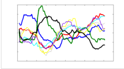
Figure 2. Average $\tau$ by sector of time: one year windows over ten years

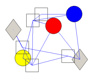
Figure 3. The network with nodes determined by $C^{2}_{\langle 2,2\rangle}$ and with distance determined by the correlation between the resulting characteristic time series. Three are identified by sector (red=Basic Materials, yellow=Services, blue=Financial) while the two diamond shaped clusters are classified by inter-sector commonalities as described in the text.

Table 1. Classification of clusters from Figure 3

Number	Classification
Technology Cluster
1	Application/Business Software
2	Semiconductor Equipment/Materials
3	Semiconductor manufacture
4	Network and Communication Devices
5	China/India based internet/
	wireless/online community companies

Table 2. Classification of clusters of $C^{1}_{\langle 1,*\rangle}$ and $C^{1}_{\langle 2,*\rangle}$

Cluster∗	Sector†	Classification
(1,1)	N	None
(2,6)	N	None
(3,2)	N	None
(4,1)	N	None
(5,1)	N	None
(6,7)	F	Closed End Funds
(7,3)	N	None
(8,3)	T	IT Products/Services
(9,6)	F	Regional Banking, S&Ls
(10,7)	F	Closed-End Funds, Debt
(11,6)	N	None
(12,1)	S	Strip Mall Stores
(13,7)	F	REITs
(14,4)	N	EU countries
(15,5)	B	Oil ans Gas
(16,3)	T	Semiconductors,
		Electronics
(17,6)	F	Regional Banking, S&Ls
(18,2)	H	Biotechnology
(19,1)	N	Entertainment/Leisure
(20,7)	F	Regional Banking
(21,3)	T	Software
(22,1)	I	Construction
(23,7)	F	Insurance
(24,2)	H	Drugs/Medical Supplies
(25,1)	B	Chemicals

^∗ The cluster is recorded as $(a,b)$ where $a$ is the $C^{1}_{\langle 1,*\rangle}$ label and $b$ is the $C^{1}_{\langle 2,*\rangle}$ label.
^† Sectors are identified via Yahoo! Finance labels as B (Basic Materials), C (Consumer Goods), F (Financial), H (Healthcare), I (Industrial Goods), N (None), S (Services), T (Technology), and U (Utilities)

Table 3. Classification of clusters of $C^{1}_{\langle 1,*\rangle}$ and $C^{1}_{\langle 2,*\rangle}$ (continued)

Cluster∗	Sector†	Classification
(26,7)	U	Electric
(27,5)	B	Industrial Metals
(28,3)	T	Scientific/Technical
		Instruments
(29,1)	C	Grocery Store Items
(30,3)	T	Communication
(31,4)	N	China and India
(32,4)	N	Latin America, Non-EU
		European countries
(33,3)	T	Computer components
(34,1)	S	Media Companies
(35,7)	F	Brokerages, Asset/
		Credit Management
(36,3)	T	None
(37,5)	B	Oil and Gas Drilling
(38,2)	H	Health Care Plans
(39,1)	S	Shipping - Air and Rail
(40,7)	U	Gas
(41,1)	S	Restaurants
(42,3)	T	Internet Services
(43,1)	I	Aerospace
		Products/Services
(44,4)	N	Brazil
(45,1)	C	Auto Parts/
		Manufacture
(46,7)	N	Canada
(47,4)	N	Japan
(48,1)	I	Res. Construction
(49,5)	B	Gold Industries

^∗ The cluster is recorded as $(a,b)$ where $a$ is the $C^{1}_{\langle 1,*\rangle}$ label and $b$ is the $C^{1}_{\langle 2,*\rangle}$ label.
^† Sectors are identified via Yahoo! Finance labels as B (Basic Materials), C (Consumer Goods), F (Financial), H (Healthcare), I (Industrial Goods), N (None), S (Services), T (Technology), and U (Utilities)

References

- [1] E. Kandel, J. Schwartz and T. Jessell, “Principles of Neural Science”, McGraw-Hill, New York, 2000.
- [2] D. J. Watts, R. Muhamad, D. C. Medina and P.S. Dodds, “Multiscale, resurgent epidemics ina hierarchical metapopulation model”, Proc. Natl. Acad. Sci. 102, pp. 11157–11162 (2005).
- [3] D. J. Watts, P.S. Dodds and M. E. J. Newman, “Identity and Search in Social Networks”, Science 296, pp. 1302 – 1305 (2002).
- [4] A. Broder, R. Kumar, F. Maghoul, P. Raghavan, S. Rajagopalan, R. Stat, A. Tomkins and J. Wiener, “Graph structure in the Web”, Computer Networks 33 pp. 309–320 (2000).
- [5] P. A. Gompers and A, Metrick, “Institutional Investors and Equity Prices”,Quarterly Journal of Economics 116:1, pp. 229–259 (2001).
- [6] Khandani, Amir E. and Lo, Andrew W., ”What Happened to the Quants in August 2007?” (November 4, 2007). Available at SSRN: http://ssrn.com/abstract=1015987
- [7] S. G. Mallat, “A theory for multiresolution signal decomposition: The wavelet representation,” IEEE Trans. Pattern Anal. Machine Intell., 11, pp. 674–693 (1989).
- [8] P. E. Barbano, , M. Spivak , J. Feng, M. Antoniotti , and B. Mishra, “A coherent framework for multiresolution analysis of biological networks with ‘memory’: Ras pathway, cell cycle, and immune system,” Proc. Natl. Acad. Sci. 102, pp. 6245–6250 (2005).
- [9] I. Rahman, I. Drori, V. C. Stodden, D. L. Donoho, and P. Schroeder, “Multiscale representations for manifold valued data,” SIAM Journal on Multiscale Modeling and Simulation, pp. 1201-1232 (2005).
- [10] J. Hair, R. L. Tatham, R. E. Anderson, and W. Black Multivariate Data Analysis, Prentice Hall, NJ (2004).
- [11] R. N. Mantegna, “Hierarchical structure in financial markets,” Eur. Phys. J. B, pp. 193–197 (1999).
- [12] M. Tumminello, T. Aste, T. Di Matteo and R. N. Mantegna, “A tool for filtering information in complex systems,” Proc. Natl. Acad. Sci. 102, pp. 10421–10426 (2005).
- [13] V. Plerou, P. Gopikrishnan, B. Rosenow, L.A.N. Amaral, T. Guhr, and H. E. Stanley, “A Random Matrix approach to Financial Cross-Correlations” Phys. Rev. E 66, 066126 (2002).
- [14] V. Plerou, P. Gopikrishnam, B. Rosenow, L. Amaral and H. E. Stanley, “Universal and non-universal properties of cross-correlations in financial time series,” Phys. Rev. Letters, p. 1471 (1999).
- [15] H. E. Stanley, L. A. N. Amaral, S. V. Buldyrev, P. Gopikrishnan, V. Plerou, and M. A. Salinger, “Self-Organized Complexity in Economics and Finance,” Proc. Natl. Acad. Sci. 99-Supp, pp.2561-2565 (2002)
- [16] D. H. Kim and H. Jeong “Systematic analysis of group identification in stock markets,” Phys. Rev. E 72, 046133 (2005).
- [17] A. Ng, M. Jordan and Y. Weiss. “On spectral clustering: Analysis and an algorithm”, In Advances in Neural Information Processing Systems 14: Proceedings of the 2001.
- [18] R. O. Duda, P. E. Hart and D. G. Stork “Pattern Clasification”, Wiley Interscience, New York, 1996.
- [19] John J. Murphy, “Intermarket Analysis: Profiting from global market relationships”, John Wiley and Sons, New York 2004. pp.200-215.
- [20] Afra Zomorodian and Gunnar Carlsson, “Computing persistent homology”, SCG ’04: Proceedings of the twentieth annual symposium on Computational geometry, pp. 347-356 (2004).
- [21] Robert Ghrist, “Barcodes: The persistent topology of data”, Bull. Amer. Math. Soc. 45 pp. 61-75 (2008);