How to quantify the influence of correlations on investment diversification

Abstract

When assets are correlated, benefits of investment diversification are reduced. To measure the influence of correlations on investment performance, a new quantity—the effective portfolio size—is proposed and investigated in both artificial and real situations. We show that in most cases, the effective portfolio size is much smaller than the actual number of assets in the portfolio and that it lowers even further during financial crises.

, ,

1 Introduction

Investment optimization, pioneered by Markowitz (Markowitz, 1952), is one of the key topics in finance. It aims at simultaneous maximization of the investor’s capital and minimization of the risk of unfavorable events. When these goals are mathematically formalized, they give rise to various methods of portfolio optimization. In this paper we focus on the Mean–Variance method (Markowitz, 1952) and the maximization of the expected exponential growth rate (Kelly, 1956). For a thorough review of modern portfolio theory see (Elton et al., 2006).

Most portfolio optimization strategies result in investment diversification as it allows investors to decrease their exposure to the risk of single assets (Lintner, 1965). In consequence, diversification represents a major issue in modern finance theory and practice (Markowitz, 1991). The basic premise is that with sufficient diversification one is able to reduce fluctuations to an acceptable level. However, when assets are correlated, the improvement of investment performance achieved by diversification is reduced (Elton & Gruber, 1977). Since asset correlations are ubiquitous, ranging from correlations between stocks in one stock market (Statman, 1987) to correlations between different investment types in different countries (Jorion, 1985; Meric et al., 2008; Olibe et al., 2008), it is important to investigate their influence on diversified portfolios (Heston & Rouwenhorst, 1994; Polkovnichenko, 2005). Worse, during financial crises like the one we currently endure, we often observe that when we need diversification the most it often fails us, leading to massive losses (Scholes, 2000).

In this paper we attempt to quantify how correlations reduce the benefits of diversification. To achieve this we propose a new measure, the effective size of a diversified portfolio, which is based on a comparison with a fictitious portfolio of uncorrelated assets. We apply this idea for two different optimization strategies (the Mean–Variance portfolio and the Kelly portfolio) and obtain analytical expressions for their effective sizes. We show that this number is often small, even for a portfolio constructed from a very large number of stocks. The achieved results are also used to study real market data (daily prices of stocks from the Dow Jones Industrial Average and the S&P 500), showing that the effective portfolio size varies significantly for different sets of stocks and different times.

2 Correlations and the Mean–Variance portfolio

First we introduce the notation used in this paper. If the initial and final asset values are $w_{0}$ and $w_{1}$ respectively, the asset return during the given time period is defined as $R:=(w_{1}-w_{0})/w_{0}$. If we follow the value of asset $i$ over many subsequent time periods, it is possible to define the average return $\mu_{i}:=\langle R_{i}\rangle$, the return variance $V_{i}:=\langle R_{i}^{2}\rangle-\langle R_{i}\rangle^{2}$ and the standard deviation $\sigma_{i}:=\sqrt{V_{i}}$ ($\langle x\rangle$ denotes the average value of $x$). To measure correlations of returns, the Pearson’s formula is the standard tool. For assets $i$ and $j$ it reads

$$C_{ij}:=\frac{\langle R_{i}R_{j}\rangle-\langle R_{i}\rangle\langle R_{j}\rangle}{\sigma_{i}\sigma_{j}},$$ (1)

by definition $C_{ij}\in[-1;1]$ and $C_{ii}=1$. When returns $R_{i}$ and $R_{j}$ are independent, $\langle R_{i}R_{j}\rangle=\langle R_{i}\rangle\langle R_{j}\rangle$ and hence $C_{ij}=0$. The same holds when one of the assets is risk-free, i.e. its return has zero variance. (Although in practice each investment carries a certain amount of risk, short term government-issued securities are often used as proxies for risk-free assets.) We assume that a risk free asset is available and has zero return. Correlation values of all assets form the correlation matrix $\mathsf{C}$.

To construct a portfolio, the investor has to divide the current wealth $W$ among $M$ available assets. This division can be characterized by investment fractions: $f_{i}$ is the fraction of wealth invested in asset $i$ ($i=1,\dots,M$). Assuming unit initial wealth, after one time period the investor has wealth

$$W_{1}=1+\sum_{i=1}^{M}f_{i}R_{i}.$$ (2)

Here $R_{i}$ is the return of asset $i$ during the period. When investment fractions are fixed, the investor’s wealth follows a multiplicative stochastic process and after $T$ periods it becomes

$$W_{T}=\prod_{t=1}^{T}\Big{(}1+\sum_{i=1}^{M}f_{i}R_{i,t}\Big{)}.$$ (3)

Here $R_{i,t}$ is the return of asset $i$ in the period $t$.

The Mean–Variance approach to portfolio optimization has been proposed by Markowitz (Markowitz, 1952), for later discussions see (Merton, 1972; Markowitz, 1991; Elton et al., 2006). Despite its flaws (e.g., only the expected return and its variance are used to characterize a portfolio) it is still a benchmark for other optimization methods. For any portfolio, we can compute the expected return $R_{P}:=\langle W_{1}\rangle-1$ and the variance $V_{P}:=\langle W_{1}^{2}\rangle-\langle W_{1}\rangle^{2}$ as

$$R_{P}=\sum_{i=1}^{M}f_{i}\mu_{i},\quad V_{P}=\sum_{i,j=1}^{M}f_{i}f_{j}C_{ij}\sigma_{i}\sigma_{j}.$$ (4)

The optimal portfolio is defined as the one that minimizes $V_{P}$ for a given $R_{P}$ (equivalently, one can maximize $R_{P}$ with $V_{P}$ fixed). To focus purely on the influence of correlations on the optimization process, we assume that all $M$ games are identical: $\mu_{i}=\mu$ and $\sigma_{i}=\sigma$. The minimal portfolio variance $V_{P}^{*}$ then has the form

$$V_{P}^{*}(R_{P},M,\mathsf{C})=\frac{\sigma^{2}R_{P}^{2}}{\mu^{2}\sum_{i,j=1}^{M}(\mathsf{C}^{-1})_{ij}}$$ (5)

where $\mathsf{C}^{-1}$ is the inverse of the correlation matrix $\mathsf{C}$. The larger is the expected portfolio return, the larger is the optimal variance.

Now we look at Eq. (5) from a new perspective: we compare it with the optimal variance of the portfolio of $m$ uncorrelated assets with identical mean returns and variances which is $V_{P}^{*}(R_{P},m,\mathrm{id}_{m})$ where $\mathrm{id}_{m}$ is $m\times m$ identity matrix. We can introduce the effective size of the correlated portfolio, $m_{\text{ef}}$, by comparing the two optimal variances. The equation $V_{P}^{*}(R_{p},M,\mathsf{C})=V_{P}(R_{p},m_{\text{ef}},\mathrm{id}_{m_{\text{ef}}})$ can be solved with respect to $m_{\text{ef}}$, yielding

$$m_{\text{ef}}=\sum_{i,j=1}^{M}(\mathsf{C}^{-1})_{ij}.$$ (6)

In other words: when investing in $M$ correlated assets, the portfolio variance is the same as for $m_{\text{ef}}$ uncorrelated assets. Note that $m_{\text{ef}}$ depends only on the correlation matrix and not on the portfolio parameters $\mu,\sigma,R_{P}$. A similar sum over the elements of the inverse correlation matrix arises in the expression for the magnetic susceptibility in the Ising model (which is a prominent model of magnetism in theoretical physics).

To better understand the new concept, we examine the special case of uniform correlations between the assets: $C_{ij}=C$ for $i\neq j$, $C\in[0;1]$. Then $\mathsf{C}^{-1}$ has the form

$$(\mathsf{C}^{-1})_{ii}=\frac{1+(M-2)C}{(1-C)[1+(M-1)C]},\quad(\mathsf{C}^{-1})_{ij}=\frac{-C}{(1-C)[1+(M-1)C]}.$$ (7)

and Eq. (6) consequently simplifies to

$$m_{\text{ef}}=\frac{M}{1+(M-1)C}.$$ (8)

Now we can get some intuition about the effective portfolio size: when $C=1$ (perfectly correlated assets), $m_{\text{ef}}=1$; when $C=0$ (uncorrelated assets), $m_{\text{ef}}=M$; when $C=-1$ and $M=2$, the portfolio variance can be totally eliminated and $m_{\text{ef}}\to\infty$. A remarkable consequence of Eq. (8) is that in the limit $M\to\infty$ we obtain $m_{\text{ef}}=1/C$. This means that diversification into arbitrary many assets with mutual correlation $C$ is equivalent to investment in only $1/C$ uncorrelated assets.

Another interesting case is a block diagonal matrix $\mathsf{C}$ which has square matrices $\mathsf{C}_{1},\dots,\mathsf{C}_{N}$ along the main diagonal and the off-diagonal blocks are zero matrices (such a form of $\mathsf{C}$ is an extreme case of the sector structure discussed in Sec. 3.3). It can be shown that Eq. (6) then yields

$$m_{\text{ef}}=m_{\text{ef}}(\mathsf{C}_{1})+\dots+m_{\text{ef}}(\mathsf{C}_{N}).$$ (9)

Thus, the effective portfolio size is the sum of effective sizes for each block $\mathsf{C}_{i}$ separately.

It is instructive to compare the results obtained above with the simple investment distributed evenly among all assets. If we assume identical returns and variances of the assets, Eq. (4) simplifies to $R_{P}=Mf\mu$, $V_{P}=\sigma^{2}f^{2}\sum_{i,j=1}^{M}C_{ij}$, where $f$ is the fraction of wealth invested in each single asset. The desired value of $R_{P}$ now determines both $f$ and $V_{P}$. By comparison with the variance of a portfolio of uncorrelated assets we obtain the effective size of the even investment in the form

$$m_{\text{ef}}^{\prime}=\frac{M}{1+(M-1)\langle C\rangle}$$ (10)

where $\langle C\rangle$ is the average of the off-diagonal elements of $\mathsf{C}$, the prime symbol indicates that the even investment is considered. We shall see (Sec. 4) that $m_{\text{ef}}^{\prime}$ is often significantly smaller than $m_{\text{ef}}$.

We emphasize that the effective portfolio size $m_{\text{ef}}$ is different from the inverse participation ratio (also called the Herfindahl index) which is defined as $\mathrm{IPR}=1/\sum_{i=1}^{M}f_{i}^{2}$ ($f_{i}$ is the fraction of wealth invested in asset $i$). While the former quantifies the influence of correlations, the latter quantifies how unevenly wealth is distributed among the assets.

3 Correlations and the Kelly portfolio

The Kelly portfolio (Kelly, 1956) maximizes the investment performance in the long run and has several interesting mathematical properties (Browne, 2000; Finkelstein & Whitley, 1981; Thorp, 2000). Its applicability was investigated in many different situations (Markowitz, 1976; Laureti et al., 2007), including those with limited information (Whitt, 1996; Medo et al., 2008; Smimou et al., 2008), and it has been successfully used in real financial markets (Thorp, 2000). In the following paragraphs we show how the effective portfolio size can be introduce for the Kelly portfolio.

Since $W_{T}$ given by Eq. (3) follows a multiplicative random walk, investor’s wealth grows exponentially as $W_{T}=\exp[GT]$. Consequently, the long-run exponential growth rate $G$ can be written in the form

$$G:=\lim_{T\to\infty}\frac{1}{T}\ln\frac{W_{T}}{W_{0}}.$$ (11)

Maximization of this quantity is the main criterion for the construction of the Kelly portfolio. Using the law of large numbers, it can be shown that $G=\langle\ln W_{1}\rangle$ where $W_{1}$ is the wealth after one step. Assuming investment into $M$ simultaneous games we have

$$G=\bigg{\langle}\ln\Big{[}1+\sum_{i=1}^{M}f_{i}R_{i}\Big{]}\bigg{\rangle}.$$ (12)

The simplest case is one risky game with binary outcomes: $R=+1$ with the probability $p$ and $R=-1$ with the probability $1-p$. The maximization of $G$ then yields the optimal fraction

$$f^{*}=2p-1$$ (13)

which is the celebrated Kelly criterion (if short positions are not allowed, $f^{*}=0$ for $p<1/2$: it is optimal to abstain from the game). Eq. (12), allowing no analytical solution for $M\geq 5$, can be maximized by numerical techniques (Whitrow, 2007) or by analytical approximations (Medo et al., 2008) as we do below.

3.1 The effective size of the Kelly portfolio

To investigate the effect of asset correlations on the Kelly portfolio, we consider $M$ individual assets with the correlation between assets $i$ and $j$ computed by Eq. (1) and labeled as $C_{ij}$. Differentiation of Eq. (12) with respect to $f_{i}$ yields

$$\sum_{\boldsymbol{R}}\frac{P(\boldsymbol{R})R_{i}}{1+\sum_{j=1}^{M}f_{j}R_{j}}=0$$ (14)

where $P(\boldsymbol{R})$ is the probability of a given vector of returns $\boldsymbol{R}=(R_{1},\dots,R_{M})$ and the summation is over all possible $\boldsymbol{R}$ (when returns are continuous, integration must be used instead). For $M>4$, this equation has no analytical solution. Assuming that the investment return $\sum_{i=1}^{M}f_{i}R_{i}$ is small (which is plausible if the considered time period is short), we can use the expansion $1/(1+x)\approx 1-x$ to obtain

$$\sum_{j=1}^{M}f_{j}\langle R_{i}R_{j}\rangle=\langle R_{i}\rangle\qquad(i=1,\dots,M).$$ (15)

This set of linear equations gives the first approximation to $f_{i}$: when $\langle R_{i}\rangle$ and $\langle R_{i}R_{j}\rangle$ are known, the optimal investment fractions $f_{i}^{*}$ follow. A higher order expansion of $1/(1+x)$ results in higher order cross terms of returns which are generally difficult to compute.

As before, to focus on the influence of correlations we assume identical return distributions of the assets: we set $\langle R_{i}\rangle=\mu$ and $\sigma_{i}=\sigma$ for $i=1,\dots,M$, consequently $\langle R_{i}R_{j}\rangle=\mu^{2}+\sigma^{2}C_{ij}$. After substitution to Eq. (14), the optimal investment fractions are

$$\boldsymbol{f}^{*}=\frac{\mu\,(\mathsf{C}^{-1}\boldsymbol{1})}{\sigma^{2}+\mu^{2}\sum_{i,j=1}^{M}(\mathsf{C}^{-1})_{ij}}$$ (16)

where $\boldsymbol{1}$ is the $M$-dimensional vector with all elements equal to $1$. The effective portfolio size $m_{\text{ef}}$ is again obtained by a comparison with a portfolio of uncorrelated assets. One way to do this is by comparing the total invested wealth in both cases. That is, $m_{\text{ef}}$ is defined as the solution of

$$\sum_{i=1}^{M}f_{i}^{*}(M,\mathsf{C})=m_{\text{ef}}\,f^{*}(m_{\text{ef}},\mathrm{id}_{m_{\text{ef}}}).$$ (17)

Using Eq. (16) we readily obtain

$$m_{\text{ef}}=\sum_{i,j=1}^{M}(\mathsf{C}^{-1})_{ij}$$ (18)

which is exactly the same expression for $m_{\text{ef}}$ as Eq. (6) in the Mean–Variance approach. We can conclude that the effective portfolio size is a common quantity for these two optimization schemes. Nevertheless, this exact correspondence is valid only when the first order approximation is used to solve Eq. (14).

It is also possible to define the effective number of assets $m_{\text{ef}}$ differently: as the number of uncorrelated assets when the expected exponential growth rate $G(m_{\text{ef}},\mathrm{id}_{m_{\text{ef}}})$ is equal to the growth rate $G(M,\mathsf{C})$ with $M$ correlated assets. This definition is similar to the one introduced above and it also yields similar results. For practical reasons (the total investment fraction is easier to handle analytically than the exponential growth rate) we confine our analysis to the former definition.

3.2 Special case with identical correlations

Assuming identical asset correlations, $C_{ij}=C$ for $i\neq j$ ($C\in[0;1]$), Eq. (18) simplifies to

$$m_{\text{ef}}=\frac{M}{1+(M-1)C}.$$ (19)

We remind that while Eq. (8) is exact, this result is based on the first order approximation in Eq. (14). To review its accuracy, we study the problem numerically. Since with identical correlations all assets are equal, the optimal investment is distributed evenly among them. Thus, maximization of the exponential growth rate $G$ simplifies to a one-variable problem and Eq. (14) is replaced by

$$\sum_{\boldsymbol{R}}\frac{P(\boldsymbol{R})\sum_{j=1}^{M}R_{j}}{1+f\sum_{j=1}^{M}R_{j}}=0.$$ (20)

To proceed, one needs to specify the joint distribution of returns, $P(\boldsymbol{R})$. To do so we use simple assets with binary outcomes: $R_{i}=1$ (which we label as $+_{i}$) and $R_{i}=-1$ (which we label as $-_{i}$). To induce the correlations we use an artificial hidden asset $h$ with the outcome $+_{h}$ with the probability $p$ and $-_{h}$ with the probability $1-p$. Finally, asset returns are drawn conditionally on the hidden asset according to

$$P(+_{i}|+_{h})=p+(1-p)\sqrt{C},\quad P(-_{i}|-_{h})=1-p+p\sqrt{C},\quad C\in[0;1].$$ (21)

It can be shown that $P(+_{i})=p$, $P(-_{i})=1-p$, $C_{ij}=C$; thus the proposed construction satisfies our requirement of identical correlations. The distribution $P(\boldsymbol{R})$ is

$$P(\boldsymbol{R})=P(+_{h})\prod_{i=1}^{M}P(R_{i}|+_{h})+P(-_{h})\prod_{i=1}^{M}P(R_{i}|-_{h})$$ (22)

and Eq. (20) can be solved, yielding the optimal fraction $f^{*}$. Consequently, the definition relation Eq. (17) allows us to interpolate $m_{\text{ef}}$ for any $M,p,C$ (interpolation is needed because the right side of the definition equation can be numerically computed only for integer $m_{\text{ef}}$). In Fig. 1 we compare this result with Eq. (19). As can be seen, when the investment return is small ($p=0.60$ and less), the approximate result performs well. When $p=0.70$, differences appear for $C\in(0.1,0.4)$. These discrepancies are not surprising because in that region, more than 80% of wealth is invested, violating the approximation used to solve Eq. (14).

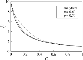
Figure 1: The effective size of the Kelly portfolio: a comparison of the approximate result Eq. (19) with numerical treatment of Eq. (20) for various winning probabilities. The total number of assets is $M=10$.

Finally, we use the established framework to investigate the effect of wrong correlation estimation on portfolio performance. We assume that all assets have pairwise correlation equal $C$ but the investor optimizes the investment assuming a different value $C^{\prime}$. In Fig. 2, the resulting growth rate $G^{*}$ is shown as a function of $C^{\prime}$. As can be seen, underestimation of correlations ($C^{\prime}<C$) decreases investment performance dramatically—a naive investor supposing zero correlations can even end up with diminishing wealth. By contrast, a similar overestimation of $C$ results in only a mild decrease of the growth rate.

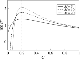
Figure 2: The optimal exponential growth rate $G^{*}$ for an investor assuming a wrong magnitude $C^{\prime}$ of asset correlation. The actual value $C=0.2$ is marked with the vertical dash-dot line, the winning probability is $p=0.55$ (i.e., $\mu=0.1$).

3.3 Estimates of the effective portfolio size

One can ask whether Eq. (18) can be approximated by a simpler formula. Motivated by Eq. (19), the natural guess is

$$m_{\text{ef}}=\frac{M}{1+(M-1)\langle C\rangle}.$$ (23)

That means, we approximate diverse correlations by their average. Since the resulting $m_{\text{ef}}$ is the same as Eq. (10): this approximation is equivalent to distributing the investment among the assets evenly.

In real markets, assets can be divided into sectors with correlations higher between assets in the same sector than between assets in different sectors. This sector structure can be used to obtain an improved estimate of $m_{\text{ef}}$. Assuming that the assets can be divided into $N$ sectors, we denote the intra-sector correlation between the assets from sector $I$ by $\tilde{C}_{II}$ and the inter-sector correlation between the assets from sectors $I$ and $J$ by $\tilde{C}_{IJ}$ (for indices labeling sectors we use capital letters). Here $\tilde{C}_{II}$ and $\tilde{C}_{IJ}$ are simple averages ($I,J=1,\dots,N$)

$$\tilde{C}_{II}=\frac{1}{M_{I}^{2}}\sum_{i,j\in I}C_{ij},\quad\tilde{C}_{IJ}=\frac{1}{M_{I}M_{J}}\sum_{i\in I,j\in J}C_{ij},$$ (24)

where $M_{I}$ is the number of assets in sector $I$. As a result, an $N$-dimensional matrix $\tilde{\mathsf{C}}$ is formed. In $\tilde{C}_{II}$ we sum also over diagonal elements of the asset correlation matrix $\mathsf{C}$ as it is convenient for our further computation.

Due to the simplifying assumption of identical intra-sector correlations, the optimal investment fractions are identical within a sector and the optimization problem simplifies to $N$ variables $f_{I}$. Similarly to Eq. (12), the exponential growth rate is

$$G=\bigg{\langle}\ln\Big{[}1+\sum_{I=1}^{N}f_{I}\sum_{i\in I}R_{i}\Big{]}\bigg{\rangle}.$$ (25)

By the same techniques as before, we obtain the estimate of the effective portfolio size

$$m_{\text{ef}}=\sum_{I,J=1}^{M}(\tilde{\mathsf{C}}^{-1})_{I,J}.$$ (26)

Its accuracy will be examined in the following section. For the Mean–Variance approach, the sector-based estimate of $m_{\text{ef}}$ is the same.

4 Correlations in real financial data

Here we test our results on real financial data, keeping two goals in mind. First, we aim to investigate actual values of the effective portfolio size. Second, we aim to examine the accuracy of $m_{\text{ef}}$ estimates derived above. We use prices of stocks from the Dow Jones Industrial Average (DJIA) and the Standard & Poor’s 500 (S&P 500) which are well-known and common indices consisting of 30 and 500 U.S. companies respectively.

4.1 Comparing index and stock variances

Using the daily data from the period 8th April 2004–14th December 2007, we compute daily returns of the DJIA and the included stocks by the formula $R(t+1)=(w(t+1)-w(t))/w(t)$, with $w(t)$ denoting the adjusted closing index value on the trading day $t$. The DJIA value is the sum of the prices of all components, divided by the Dow divisor which changes with time. This effect can be ignored because changes of the divisor are mostly negligible.

During the given period, the variance of the DJIA daily returns was $\sigma_{\mathrm{DJIA}}^{2}\approx 5.22\cdot 10^{-5}$, the average variance of the daily returns of the DJIA stocks was $\sigma_{\mathrm{S}}^{2}\approx 1.73\cdot 10^{-4}$. These two figures contradict the assumption of zero correlations because then the variance should scale with the number of assets $M$ as $1/M$ (this follows also from Eq. (5) when $\mathsf{C}=\mathrm{id}_{M}$ is substituted). By dividing $\sigma_{\mathrm{S}}^{2}/\sigma_{\mathrm{DJIA}}^{2}$ we obtain an alternative estimate of the effective number of assets (this estimate was used already in (Goetzmann & Kumar, 2004)). In our case it is equal to $3.31$ which is much less than the total number of stocks in the DJIA.

We can also estimate the effective number of assets using the results of our analysis above. From the daily stock returns, return correlations can be computed by Eq. (1), resulting in $\langle C\rangle=0.322$. Together with the number of stocks $M=30$, Eq. (23) yields $m_{\text{ef}}\approx 2.90$. This is in good agreement with the value $3.31$ obtained by a different reasoning in the previous paragraph.

4.2 The effective portfolio size

Now we compute $m_{\text{ef}}$ for the DJIA stocks described above and also for the S&P 500 index where we use the approximately 16 year period from 2nd January 1992–15th February 2008 and those 338 stocks out of the current 500 which were quoted in the stock exchange during the whole period. After the correlation matrix $\mathsf{C}$ is estimated, the effective portfolio size can be calculated using $\mathsf{C}^{-1}$ and Eq. (6) or Eq. (18), it can be approximated using a sector division and Eq. (26), or it can be approximated using $\langle C\rangle$ and Eq. (23). We use the division into nine sectors obtained from http://biz.yahoo.com/p with the industry sectors: basic materials, conglomerates, consumer goods, finance, healthcare, industrial goods, services, technology, and utilities. Using a different sector division (obtained e.g. by minimizing the ratio of average intra- and inter-sector correlations) does not influence the results substantially. To obtain the dependency of $m_{\text{ef}}$ on the portfolio size $M$, we select a random subset of $M$ stocks from the complete set and compute $m_{\text{ef}}$ for this subset; sensitivity to the subset selection is eliminated by averaging over 5 000 random draws.

Figure 3: The effective size $m_{\text{ef}}$ for the DJIA stocks (a) and the S&P 500 stocks (b), computed directly from $\mathsf{C}$, from sector division, and from $\langle C\rangle$. The estimate of the effective size obtained by comparison of variances in Sec. 4.1 is shown as a thick cross. Individual realizations fluctuate around the plotted averages with the amplitude approximately one or less.

The results of the described analysis are shown in Fig. 3. For small portfolio sizes (less than approximately ten stocks), the estimates of $m_{\text{ef}}$ based on the sector structure or on the average correlation perform well. For a larger portfolio, the sector structure gives a better description of $m_{\text{ef}}$ than the average correlation. Nevertheless, both estimates quickly saturate while $m_{\text{ef}}$ obtained from the complete correlation matrix continues to grow even for $M>100$. We see that the effect of heterogeneous correlations increases with $M$ and even the sector structure is insufficient to describe the system. The limited horizontal scale in Fig. 3 is due to noisy estimates of large correlation matrices from the data with a finite time horizon $T$. As we are determining $M(M-1)/2$ correlations from $MT$ prices, when $T$ is not very large compared to $M$, we face an underdetermined system of equations (Laloux et al., 1999) (the problem is also known as the dimensionality curse). With more frequent financial data, larger portfolios would be easily accessible.

There is one particular point to be highlighted. According to Eq. (10), the estimate of $m_{\text{ef}}$ by the average correlation $\langle C\rangle$ is equal to the effective size $m_{\text{ef}}^{\prime}$ of the portfolio containing all available assets with even weights. Such investment was investigated e.g. in (Elton & Gruber, 1977) where it was suggested that the benefits of diversification are exhausted already with a portfolio of ten assets. This result is in agreement with Fig. 3 where for both sets of stocks, the effective portfolio size based on $\langle C\rangle$ saturates at $M\approx 10$. However, since $m_{\text{ef}}^{\prime}$ is lower than the effective sizes obtained directly from a sector division and much lower than those obtained directly from $\mathsf{C}$, we can conclude that with an evenly distributed investment one cannot fully exploit the benefits of diversification.

Finally, in Fig. 4 we show the time evolution of $m_{\text{ef}}$ for twenty current stocks from the DJIA. We use the daily data from the period Jan 1973–Apr 2008 and the sliding window of one year length to obtain estimates of the correlation matrix and compute $m_{\text{ef}}$ from $\mathsf{C}^{-1}$. In the same figure we show also the average yearly return of the selected stocks (estimated on the one-year basis). As we see, $m_{\text{ef}}$ varies with a large amplitude, being as low as two at the end of 80’s (corresponding to the October crash of 1987) and peaking at almost seven during the year 1994.

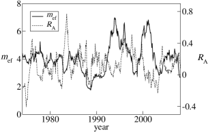
Figure 4: Time evolution of the effective size $m_{\text{ef}}$ and the average yearly stock return $R_{A}$ for the DJIA stocks, based on the sliding window of one year length. Note the three dips corresponding to the black October of 1987, the emerging market crisis of 1997, and the dot-com bubble bursting in 2001-2002.

5 Conclusion

In today’s globalized world where a single event can have world-wide implications, even internationalized portfolios are not immune to asset correlations. As a result, measurement and effects of correlations remain as a prominent challenge of portfolio theory. In this work we focused on the influence of correlations on the performance of optimal portfolios. On a simple artificial example we showed that underestimation of asset correlations can lead to a significant reduction of profitability (see Fig. 2).

Even when correlations are correctly estimated, they harm the investment performance by reducing the true degree of diversification. To measure their influence we introduced a new quantity: the effective portfolio size $m_{\text{ef}}$. We derived simple analytical expressions which allow us to easily calculate $m_{\text{ef}}$ both for the Mean–Variance portfolio and the Kelly portfolio. We showed that with increasing number of stocks, the diversification measure increases only slowly and in some cases it even saturates without any further net diversification effect. In agreement with previous studies, evenly distributed investment turns out to be a rather ineffective way of diversification as it results in relatively small values of $m_{\text{ef}}$. In addition, the time dependence of $m_{\text{ef}}$ obtained from prices of the DJIA stocks shows strong its heavy variations and also minima corresponding to the crashes that occurred in the investigated period.

Although illustrated only on the Mean–Variance portfolio and the Kelly portfolio, the effective portfolio size is a general concept which can be used also in other optimization methods. It reduces the complex structure of the full correlation matrix to a single number with a simple interpretation and thus it allows us to appreciate how much do correlations harm our investment. In future research, numerical results for $m_{\text{ef}}$ should be refined using high frequency financial data which would allow for shorter sliding window lengths and fewer averaging artifacts. Since correlation estimates are noisy even with extensive data available, it would be interesting to see how the concept of the effective size applies to a noisy correlation matrix. Eventual direct applications of the proposed concept to portfolio management remain as a future challenge.

References

- Browne (2000) Browne, S. (2000). Can you do better than Kelly in the short run? in Finding the Edge, Mathematical Analysis of Casino Games, eds. O. Vancura, J. Cornelius, & W. R. Eadington, University of Nevada.
- Elton & Gruber (1977) Elton, E. J., & Gruber, M. J. (1977). Risk Reduction and Portfolio Size: An Analytical Solution. The Journal of Business, 50, 415–437.
- Elton et al. (2006) Elton, E. J., Gruber, M. J., Brown, S. J., & Goetzmann, W. N. (2006). Modern Portfolio Theory and Investment Analysis, 7th Edition, Wiley, New York.
- Finkelstein & Whitley (1981) Finkelstein, M., & Whitley, R. (1981). Optimal Strategies for Repeated Games. Advances in Applied Probability, 13, 415–428.
- Goetzmann & Kumar (2004) Goetzmann, W. N., & Kumar, A. (2004). Why do individual investors hold under-diversified portfolios? working paper.
- Heston & Rouwenhorst (1994) Heston, S. L., & Rouwenhorst, K. G. (1994). Does Industrial Structure Explain the Benefits of International Diversification? Journal of Financial Economics, 36, 3–27.
- Jorion (1985) Jorion, P. (1985). International Portfolio Diversification with Estimation Risk. The Journal of Business, 58, 259–278.
- Kelly (1956) Kelly, J. L. (1956). A new interpretation of information rate. IEEE Transactions on Information Theory, 2, 185–189.
- Laloux et al. (1999) Laloux, L., Cizeau, P., Bouchaud, J.-P., Potters, M. (1999). Noise dressing of Financial Correlation Matrices. Phys. Rev. Lett., 83, 1467–1470.
- Laureti et al. (2007) Laureti, P., Medo, M., & Zhang, Y.-C. (2007). Analysis of Kelly-optimal portfolios. arXiv:0712.2771.
- Lintner (1965) Lintner, J. (1965). Security Prices, Risk, and Maximal Gains From Diversification. The Journal of Finance, 20, 587–615.
- Markowitz (1952) Markowitz, H. M. (1952). Portfolio Selection. The Journal of Finance, 7, 77–91.
- Markowitz (1976) Markowitz, H. M. (1976). Investment for the Long Run: New Evidence for an Old Rule. The Journal of Finance, 31, 1273–1286.
- Markowitz (1991) Markowitz, H. M. (1991). Portfolio Selection: Efficient Diversification of Investments, Wiley, New York.
- Medo et al. (2008) Medo, M., Pis’mak,Y. M., & Zhang, Y.-C. (2008). Diversification and limited information in the Kelly game. Physica A, 387, 6151–6158.
- Meric et al. (2008) Meric, I., Ratner, M., & Meric, G. (2008). Co-movements of sector index returns in the world’s major stock markets in bull and bear markets: Portfolio diversification implications. International Review of Financial Analysis, 17, 156–177.
- Merton (1972) Merton, R. C. (1972). An Analytic Derivation of the Efficient Portfolio Frontier. The Journal of Financial and Quantitative Analysis, 7, 1851–1872.
- Olibe et al. (2008) Olibe, K. O., Michello, F. A., & Thorne, J. (2008). Systematic risk and international diversification: An empirical perspective. International Review of Financial Analysis, 17, 681–698.
- Polkovnichenko (2005) Polkovnichenko, V. (2005). Household Portfolio Diversification: A Case for Rank-Dependent Preferences. Review of Financial Studies, 18, 1467–1502.
- Scholes (2000) Scholes M. S. (2000). Crisis and Risk Management. American Economic Review, 90, 17–21.
- Smimou et al. (2008) Smimou, K., Bector, C. R., & Jacoby, G. (2008). Portfolio selection subject to experts’ judgments International Review of Financial Analysis, 17, 1036–1054.
- Statman (1987) Statman, M. (1987). How Many Stocks Make a Diversified Portfolio? The Journal of Financial and Quantitative Analysis, 22, 353–363.
- Thorp (2000) Thorp, E. O. (2000). The Kelly criterion in Blackjack, sports betting, and the stock market. in Finding the Edge, Mathematical Analysis of Casino Games, eds. O. Vancura, J. Cornelius, & W. R. Eadington, University of Nevada.
- Whitt (1996) Browne, S., & Whitt, W. (1996). Portfolio choice and the Bayesian Kelly criterion. Adv. Appl. Prob., 28, 1145–1176.
- Whitrow (2007) Whitrow, C. (2007). Algorithms for optimal allocation of bets on many simultaneous events. Appl. Statist., 56, 607–623.