Detecting single-electron tunneling involving virtual processes in real time

Abstract

We use time-resolved charge detection techniques to probe virtual tunneling processes in a double quantum dot. The process involves an energetically forbidden state separated by an energy $\delta$ from the Fermi energy in the leads. The non-zero tunneling probability can be interpreted as cotunneling, which occurs as a direct consequence of time-energy uncertainty. For small energy separation the electrons in the quantum dots delocalize and form molecular states. In this regime we establish the experimental equivalence between cotunneling and sequential tunneling into molecular states for electron transport in a double quantum dot. Finally, we investigate inelastic cotunneling processes involving excited states of the quantum dots. Using the time-resolved charge detection techniques, we are able to extract the shot noise of the current in the cotunneling regime.

I Introduction

A semiconductor double quantum dot (DQD) is the mesoscopic analogue of a diatomic molecule. The energy levels and the interdot coupling energy can be precisely controlled with gate voltages van der Wiel et al. (2002), which allows the DQD to be tuned to a configuration where the electron wavefunctions hybridize and form molecular states extending over both QDs. The DQD thus provides a tunable two-level system, which has been utilized to perform coherent manipulation of a single charge in semiconductor nanostructures Hayashi et al. (2003); Petta et al. (2004).

An alternative approach to molecular states at large detuning is to study electron transport in the DQD in the framework of cotunneling Golovach and Loss (2004). Cotunneling involves an electron (or hole) that virtually tunnels through an energetically forbidden charge state of the QD positioned at an energy $\delta$ away from the Fermi energy in the leads. The process occurs on a timescale $\tau_{\mathrm{cot}}\sim\hbar/\delta$ limited by time-energy uncertainty Averin and Nazarov (1990). Cotunneling currents are generally small and difficult to measure, but the effect has been utilized for QD spectroscopy De Franceschi et al. (2001); Zumbühl et al. (2004), for studying cotunneling-mediated transport in single QDs Schleser et al. (2005), or for investigating spin effects in double QDs Liu et al. (2005).

In this work we use a quantum point contact (QPC) as a charge sensor Field et al. (1993) to detect single-electron tunneling in the DQD in real-time Fujisawa et al. (2004); Schleser et al. (2004); Vandersypen et al. (2004). Similar setups have been used for investigating single-spin dynamics Elzerman et al. (2004), detecting single-particle interference Gustavsson et al. (2008a), probing interactions between charge carriers Gustavsson et al. (2006a) or for measuring extremely small currents Fujisawa et al. (2006); Gustavsson et al. (2008b). Here, we utilize the technique to count electrons cotunneling through the DQD. The method provides a precise measurement of the tunneling probability as a function of energy separation $\delta$ between the QDs, allowing a direct comparison with the rate expected from time-energy uncertainty. In the limit of $\delta\rightarrow 0$, the electrons form molecular states extending over both QDs. Here, we measure tunneling rates expected from sequential tunneling into bonding and antibonding states of the DQD. The results experimentally establish the equivalence between cotunneling into coupled QD states and sequential tunneling into molecular states of the DQD.

In the last part of the paper we investigate inelastic cotunneling processes involving excited states of the DQD. Finally, we use the time-resolved charge-detection techniques to extract the shot noise of the DQD current in the cotunneling regime.

II Experimental setup and methods

The measurements were performed on the structure shown in Fig. 1(a). The sample is fabricated with local oxidation Fuhrer et al. (2002) of a GaAs/Al_0.3Ga_0.7As heterostructure, containing a two-dimensional electron gas (2DEG) 34 nm below the surface. The structure consists of two QDs (marked by 1 and 2 in the figure) connected by two separate tunnel barriers. Each QD contains about 30 electrons. For the results presented here only the upper tunnel barrier was kept open; the lower was pinched-off by applying appropriate voltages to the surrounding gates. The sample details are described in Ref. Gustavsson et al. (2007).

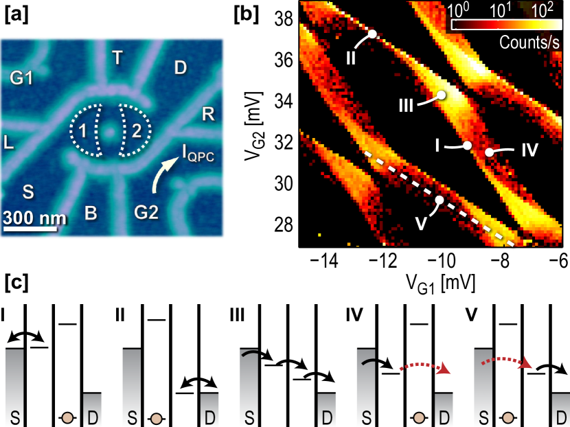
Figure 1: (a) AFM-image of the sample. The structure consists of a double quantum dot (DQD) (marked by 1 and 2) with a near-by quantum point contact. (b) Charge stability diagram of the DQD, measured by counting electrons entering and leaving the DQD. The data was taken with a voltage bias of $V_{\mathrm{DQD-SD}}=600\,\mu\mathrm{V}$ applied over the DQD. The QPC conductance was measured with $V_{\mathrm{QPC-SD}}=300\,\mu\mathrm{V}$. The count rates were extracted from traces of length $T=0.5\,\mathrm{s}$. (c) Energy level diagrams for different configurations in (b).

The electron population of the DQD is monitored by operating the QPC in the lower-right corner of Fig. 1(a) as a charge detector Field et al. (1993). By tuning the tunneling rates of the DQD below the detector bandwidth, charge transitions can be detected in real-time Vandersypen et al. (2004); Schleser et al. (2004); Fujisawa et al. (2004). In the experiment, the tunneling rates $\Gamma_{\mathrm{S}}$ and $\Gamma_{\mathrm{D}}$ to source and drain leads are kept around 1 kHz, while the interdot coupling $t$ is set much larger ($t\sim 20\,\mu\mathrm{eV}\sim 5~{}\mathrm{GHz}$). Interdot transitions thus occur on timescales much faster than it is possible to register with the detector ($\tau_{\mathrm{det}}\sim 50\,\mathrm{\mu s}$) Naaman and Aumentado (2006), but the coupling energy may still be determined from charge localization measurements DiCarlo et al. (2004). The conductance of the QPC was measured by applying a bias voltage of $200-400\,\mu\mathrm{V}$ and monitoring the current [$I_{\mathrm{QPC}}$ in Fig. 1(a)]. We ensured that the QPC bias voltage was kept low enough to avoid charge transitions driven by current fluctuations in the QPC Gustavsson et al. (2007). The sample is realized without metallic gates so that the coupling between dots and QPC detectors is not screened by metallic structures.

Figure 1(b) shows a charge stability diagram for the DQD, measured by counting electrons tunneling into and out of the DQD. The data was taken with a bias voltage of $600\,\mu\mathrm{V}$ applied across the DQD, giving rise to finite-bias triangles of sequential transport van der Wiel et al. (2002). The diagrams in Fig. 1(c) show schematics of the DQD energy levels for different positions in the charge stability diagram. Depending on energy level alignment, different kinds of electron tunneling are possible.

At the position marked by I in Fig. 1(b), the electrochemical potential $\mu_{\mathrm{1}}$ of QD1 is aligned with the Fermi level of the source lead. The tunneling is due to equilibrium fluctuations between source and QD1. A measurement of the count rate as a function of $\mu_{\mathrm{1}}$ provides a way to determine both the tunneling rate $\Gamma_{\mathrm{S}}$ and the electron temperature in the source lead Gustavsson et al. (2006b). The situation is reversed at point II in Fig. 1(b). Here, electron tunneling occurs between QD2 and the drain, thus giving an independent measurement of $\Gamma_{\mathrm{D}}$ and the electron temperature of the drain lead. At point III within the triangle of Fig. 1(b), the levels of both QD1 and QD2 are within the bias window and the tunneling is due to sequential transport of electrons from the source lead into QD1, over to QD2 and finally out to the drain. The electron flow is unidirectional and the count rate relates directly to the current flowing through the system Fujisawa et al. (2006). Between the triangles, there are broad, band-shaped regions with low but non-zero count rates where sequential transport is expected to be suppressed due to Coulomb blockade [cases IV and V in Fig. 1(b,c)]. The finite count rate in this region is attributed to electron tunneling involving virtual processes. These features will be investigated in more detail in the forthcoming sections.

To begin with, we use the time-resolved charge detection methods to characterize the system. Typical time traces of the QPC current for DQD configurations marked by I and II in Fig. 1(b) are shown in Fig. 2(a). The QPC current switches between two levels, corresponding to electrons entering or leaving QD1 (case I) or QD2 (case II). The change $\Delta I_{\mathrm{QPC}}$ as one electron enters the DQD is larger for charge fluctuations in QD2 than in QD1. This reflects the stronger coupling between the QPC and QD2 due to the geometry of the device. A measurement of $\Delta I_{\mathrm{QPC}}$ thus gives information about the charge localization in the DQD.

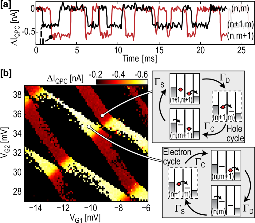
Figure 2: (a) Typical time traces of the QPC current from configurations I and II in Fig. 1(b). (b) Change of QPC current $\Delta I_{\mathrm{QPC}}$ as one electron enters the DQD, extracted from the same set of data as shown in Fig. 1. The two levels correspond to the QPC detector registering electron tunneling in QD1 and QD2, respectively. The energy level diagrams describe the hole and the electron cycle of sequential transport within the finite bias triangles.

In Fig. 2(b) we investigate the charge localization in more detail by plotting the absolute change in QPC current $\Delta I_{\mathrm{QPC}}$ for the same set of data as in Fig. 1(a). The detector essentially only measures two different values of $\Delta I_{\mathrm{QPC}}$; either $\Delta I_{\mathrm{QPC}}\sim-0.3\,\mathrm{nA}$ or $\Delta I_{\mathrm{QPC}}\sim-0.6\,\mathrm{nA}$. Comparing the results of Fig. 2(b) with the sketches in Fig. 1(c), we see that regions with high $\Delta I_{\mathrm{QPC}}$ match with the regions where we expect the counts to be due to electron tunneling in QD2, while the regions with low $\Delta I_{\mathrm{QPC}}$ come from electron tunneling in QD1.

The regions inside the bias triangles are described in detail in the energy level diagrams of Fig. 2(b). We assume each QD to hold n and m electrons, respectively. In the lower triangle, the current is carried by a sequential electron cycle. Starting from the (n,m)-configuration, an electron will tunnel in from the source lead at a rate $\Gamma_{\mathrm{S}}$ making the transition $(\mathrm{n,m})\rightarrow(\mathrm{n+1,m})$. The electron then passes on to QD2 at a rate $\Gamma_{\mathrm{C}}\sim t/h$ $[(\mathrm{n+1,m})\rightarrow(\mathrm{n,m+1})]$ before leaving to drain at the rate $\Gamma_{\mathrm{D}}$ $[(\mathrm{n,m+1})\rightarrow(\mathrm{n,m})]$. Since the rate $\Gamma_{\mathrm{C}}$ is much faster than the detector bandwidth (and $\Gamma_{\mathrm{C}}\gg\Gamma_{\mathrm{S}},~{}\Gamma_{\mathrm{C}}\gg\Gamma_{\mathrm{D}}$), the detector will only register transitions between the two states $(\mathrm{n,m})$ and $(\mathrm{n,m+1})$. Therefore, we expect the step height $\Delta I_{\mathrm{QPC}}$ within the lower triangle to be equal to $\Delta I_{\mathrm{QPC}}$ measured for electron fluctuations in QD2, in agreement with the results of Fig. 2.

For the upper triangle, the DQD holds an additional electron and the current is carried by a hole cycle. Starting with both QDs occupied $[(\mathrm{n+1,m+1})]$, an electron in QD2 may leave to the drain $[(\mathrm{n+1,m+1})\rightarrow(\mathrm{n+1,m})]$, followed by a fast interdot transition from QD1 to QD2 $[(\mathrm{n+1,m})\rightarrow(\mathrm{n,m+1})]$. Finally, an electron can tunnel into QD1 from the source lead $[(\mathrm{n,m+1})\rightarrow(\mathrm{n+1,m+1})]$. In the hole cycle, the detector is not able to resolve the time the system stays in the $(\mathrm{n+1,m})$ state; the measurement will only register transitions between $(\mathrm{n+1,m+1})$ and $(\mathrm{n,m+1})$. This corresponds to fluctuations of charge in QD1, giving the low value of $\Delta I_{\mathrm{QPC}}$ in Fig. 2(b). Finally, we note that at the transition between regions of low and high $\Delta I_{\mathrm{QPC}}$ the electron wavefunction delocalizes onto both QDs. This provides a method for determining the interdot coupling energy $t$ DiCarlo et al. (2004). From the data in Fig. 2(b) we find tunnel couplings in the range of $10-50\,\mu\mathrm{eV}$.

III Cotunneling

We now focus on the regions of weak tunneling occuring in regions outside the boundaries expected from sequential transport. In case IV, the electrochemical potential of QD1 is within the bias window, but the potential of QD2 is shifted below the Fermi level of the source and not available for transport. We attribute the non-zero count rate for this configuration to be due to electrons cotunneling from QD1 to the drain lead. The time-energy uncertainty principle still allows electrons to tunnel from QD1 to drain by means of a higher order process. In case V, the situation is analogous but the roles of the two QDs are reversed; electrons cotunnel from the source into QD2 and leave sequentially to the drain lead.

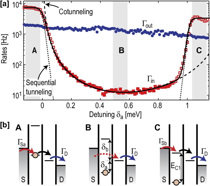
Figure 3: Tunneling rates for electrons entering and leaving the DQD, measured while keeping the potential of QD2 fixed and sweeping the electrochemical potential of QD1. The data is measured in a configuration similar to going along the dashed line in Fig. 1(b). The dotted lines are tunneling rates expected from sequential tunneling, while the dashed line is a fit to the cotunneling model of Eq. (1). The solid line corresponds to the model involving molecular states [Eq. (5)]. Parameters are given in the text. (b) Schematic drawings of the DQD energy levels for three different configurations in (a). At point A, electrons tunnel sequentially through the structure. Moving to point B, the energy levels of QD1 are shifted and the electron in QD1 is trapped due to Coulomb blockade. Electron transport from source to QD2 is still possible through virtual processes, but the rate for electrons entering the DQD drops substantially due to the low probability of the virtual processes. At point C, the next level of QD1 is brought inside the bias window and sequential transport is again possible.

To investigate the phenomenon more carefully, we measure the rates for electrons tunneling into and out of the DQD in a configuration similar to the configuration along the dashed line in Fig. 1(b). The line corresponds to keeping the electrochemical potential of QD2 fixed within the bias window and sweeping $\mu_{1}$. The data is presented in Fig. 3. In the region marked by A in Fig. 3, electrons tunnel sequentially from source into QD1, relax from QD1 down to QD2 and finally tunnel out from QD2 to the drain lead. Proceeding from region A to region B, the electrochemical potential $\mu_{1}$ is lowered so that an electron eventually gets trapped in QD1. At point B, the electrons lack an energy $\delta_{a}=\mu_{2}-\mu_{1}$ to leave to QD2. Still, electron tunneling is possible by means of a virtual process Averin and Nazarov (1990). Due to the energy-time uncertainty principle, there is a time-window of length $\sim\!\hbar/\delta_{a}$ within which tunneling from QD1 to QD2 followed by tunneling from the source into QD1 is possible without violating energy conservation. An analogous process is possible involving the next unoccupied state of QD1, occuring on timescales $\sim\!\hbar/\delta_{b}$, where $\delta_{b}=E_{\mathrm{C1}}-\delta_{a}$ and $E_{C1}$ is the charging energy of QD1. The two processes correspond to electron cotunneling from the source lead to QD2. Continuing from point B to point C, the unoccupied state of QD2 is shifted into the bias window and electron transport is again sequential.

In the sequential regime (regions A and C), we fit the rate for electrons entering the DQD to a model involving only sequential tunneling [dotted lines in Fig. 3(a)] Kouwenhoven et al. (1997). The fit allows us to determine the tunnel couplings between source and the occupied ($\Gamma_{\mathrm{Sa}}$)/unoccupied ($\Gamma_{\mathrm{Sb}}$) states of QD2, giving $\Gamma_{\mathrm{Sa}}=7.5\,\mathrm{kHz}$, $\Gamma_{\mathrm{Sb}}=3.3\,\mathrm{kHz}$ and $T=100\,\mathrm{mK}$. Going towards region B, the rates due to sequential tunneling are expected to drop exponentially as the energy difference between the levels in QD1 and QD2 is increased. In the measurement, the rate $\Gamma_{\mathrm{in}}$ initially decreases with detuning, but the decrease is slower than exponential and flattens out as the detuning gets larger. This is in strong disagreement with the behavior expected for sequential tunneling. Instead, in a region around point B we attribute the measured rate $\Gamma_{\mathrm{in}}$ to be due to electrons cotunneling from source to QD2.

The rate for cotunneling from source to QD2 is given as Averin and Nazarov (1992):

$$\Gamma_{\mathrm{cot}}=\Gamma_{\mathrm{Sa}}\,\frac{t_{a}^{2}}{\delta_{a}^{2}}+\Gamma_{\mathrm{Sb}}\,\frac{t_{b}^{2}}{\delta_{b}^{2}}+\cos\phi\,\sqrt{\Gamma_{\mathrm{Sa}}\,\Gamma_{\mathrm{Sb}}}\,\frac{t_{a}\,t_{b}}{\delta_{a}\,\delta_{b}}.$$ (1)

Here, $t_{a}$, $t_{b}$ are the tunnel couplings between the occupied/unoccupied states in QD1 and the state in QD2. The first term describes cotunneling involving the occupied state of QD1, the second term describes the cotunneling over the unoccupied state and the third term accounts for possible interference between the two. The phase $\phi$ defines the phase difference between the two processes. To determine $\phi$ one needs to be able to tune the phases experimentally, which is not possible from the measurement shown in Fig. 3(a). In the following we therefore assume the two processes to be independent ($\phi=\pi/2$). Interference effects between cotunneling processes have been studied in detail in Ref. Gustavsson et al. (2008a).

The dashed line in Fig. 3(a) shows the results of Eq. (1), with fitting parameters $t_{a}=15~{}\mathrm{\mu eV}$ and $t_{b}=33~{}\mathrm{\mu eV}$. These values are in good agreement with values obtained from charge localization measurements. The values for $\Gamma_{\mathrm{Sa}}$ and $\Gamma_{\mathrm{Sb}}$ are taken from measurements in the sequential regimes. We emphasize that Eq. (1) is valid only if $\delta_{a},\delta_{b}\gg t_{a},t_{b}$ and if sequential transport is sufficiently suppressed. The data points used in the fitting procedure are marked by filled squares in the figure. It should be noted that the sequential tunneling in region C prevents investigation of the cotunneling rate at small $\delta_{b}$. This can easily be overcome by inverting the DQD bias. The rate for electrons tunneling out of the DQD [$\Gamma_{\mathrm{out}}$ in Fig. 3(a)] shows only slight variations over the region of interest. This is expected since $\mu_{2}$ stays constant over the sweep. The slight decay of $\Gamma_{\mathrm{out}}$ with increased detuning comes from tuning of the tunnel barrier between QD2 and the drain MacLean et al. (2007).

The cotunneling may be modified by the existence of a near-by QPC. If the QPC were able to detect the presence electron in QD2 during the cotunneling we would expect this to influence the cotunneling process. For the measurements in Fig. 3(a) the QPC current was kept below 10 nA. This gives an average time delay between two electrons passing the QPC of $e/I_{\mathrm{QPC}}\sim\!16~{}\mathrm{ps}$. Since this is larger than the typical cotunneling time, it is unlikely that the electrons in the QPC are capable of detecting the cotunneling process. The influence of the QPC may become important for larger QPC currents. However, when the QPC bias voltage is larger than the detuning ($eV_{\mathrm{QPC}}>\delta$), the fluctuations in the QPC current may start to drive inelastic charge transitions between the QDs Gustavsson et al. (2007); Gustavsson et al. (2008a). Such transitions will compete with the cotunneling. For this reason it was not possible to extract what effect the presence of the QPC may have on the cotunneling process.

IV Molecular states

The overall good agreement between Eq. (1) and the measured data demonstrates that time-resolved charge detection techniques provide a direct way of quantitatively using the time-energy uncertainty principle. However, a difficulty arises as $\delta\rightarrow 0$; the cotunneling rate in Eq. (1) diverges, as visualized for the dashed line in Fig. 3(a). The problem with Eq. (1) is that it only takes second-order tunneling processes into account. For small detuning $\delta$ the cotunneling described in Eq. (1) must be extended to include higher order processes Pohjola et al. (1997).

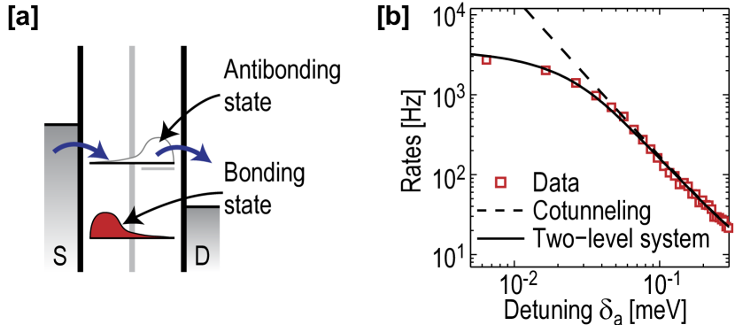
Figure 4: (a) Cotunneling described using molecular states. Due to the large detuning the empty antibonding state is mainly localized on QD2, but a small part of the wavefunction is still present in QD1 which allows an electron to enter from the source. (b) The rate for electrons tunneling into the DQD ($\Gamma_{\mathrm{in}}$) as a function of DQD detuning $\delta_{a}$. The figure shows the same data as in Fig. 3, but plotted on a log-log scale to enhance the features at small detuning. The dashed line is the results of the cotunneling model in Eq. (1), the solid line shows the result of the molecular-state model [Eq. (5)].

A different approach is to assume the coupling between the QDs to be fully coherent and describe the DQD in terms of the bonding and antibonding molecular states Gräber et al. (2006); Pedersen et al. (2007). Both the sequential tunneling and the cotunneling can then be treated as first-order tunneling processes into the molecular states; what we in Fig. 3 referred to as cotunneling would be tunneling into an antibonding state. The model is sketched in Fig. 4(a). The bonding state is occupied and in Coulomb blockade. Still, an electron may tunnel from drain into the antibonding state. Due to the large detuning, the antibonding state is mainly located on QD2, the overlap with the electrons in the source lead is small and the tunneling is weak. Changing the detuning will have the effect of changing the shape of the molecular states and shift their weights between the two QDs.

To calculate the rate for electron tunneling from source into the molecular state of the DQD as visualized in Fig. 4(a), we consider the DQD as a tunnel-coupled two-level system containing one electron, isolated from the environment. We introduce the basis states $\{\Psi_{\mathrm{1}},\Psi_{\mathrm{2}}\}$ describing the electron sitting on the left or the right QD, respectively. The two states are tunnel coupled with coupling $t$ and separated in energy by the detuning $\delta$. The Hamiltonian of the system is

$$H=\left[\begin{array}[]{cc}-\delta/2&t\\ t&\delta/2\\ \end{array}\right].$$ (2)

The eigenvectors of the Hamiltonian in Eq. (2) form the bonding $\Psi_{\mathrm{B}}$ and antibonding states $\Psi_{\mathrm{A}}$ of the system. The eigenvalues give the energies $E_{\mathrm{B}}$, $E_{\mathrm{A}}$ of the two states, with

$$E_{\mathrm{B}}=-\frac{1}{2}\sqrt{4t^{2}+\delta^{2}},~{}~{}~{}~{}E_{\mathrm{A}}=\frac{1}{2}\sqrt{4t^{2}+\delta^{2}}.$$ (3)

Note that at zero detuning there is still a finite level separation set by the tunnel coupling. The occupation probabilities $p_{\mathrm{B}}$ and $p_{\mathrm{A}}$ of the two states are determined by detailed balance,

$$p_{\mathrm{B}}=1-\frac{1}{1+e^{\frac{\sqrt{4t^{2}+\delta^{2}}}{k_{\mathrm{B}}\,T}}},~{}~{}~{}p_{\mathrm{A}}=\frac{1}{1+e^{\frac{\sqrt{4t^{2}+\delta^{2}}}{k_{\mathrm{B}}\,T}}}.$$ (4)

To calculate the rate for electrons tunneling from source into the antibonding molecular state of the DQD as visualized in Fig. 4(a), we project the thermal population $p_{\mathrm{B}}$, $p_{\mathrm{A}}$ of the molecular states $\Psi_{\mathrm{B}}$ and $\Psi_{\mathrm{A}}$ onto the unperturbed state of QD1, $\Psi_{1}$. This gives the probability $p_{1}$ of finding an electron in QD1 if making a projective measurement in the $\Psi_{1}$-basis. The measured rate $\Gamma_{\mathrm{in}}$ is equal to the probability of finding QD1 being empty $(1-p_{1})$ multiplied with $\Gamma_{\mathrm{S}}$, the tunneling rate between the source and the unperturbed state in QD1.

$$\Gamma_{\mathrm{in}} = \Gamma_{\mathrm{S}}\,(1-p_{1})=\Gamma_{\mathrm{S}}\,\left(1-(p_{\mathrm{B}}\Psi_{\mathrm{B}}+p_{\mathrm{A}}\Psi_{\mathrm{A}})\cdot\Psi_{1}\right)$$ (5)

$$= \Gamma_{\mathrm{S}}\,\frac{1}{2}\left(1-\frac{\delta\tanh\left(\frac{\sqrt{4t^{2}+\delta^{2}}}{2k_{\mathrm{B}}\,T}\right)}{\sqrt{4t^{2}+\delta^{2}}}\right)$$

For large detuning, the bonding and antibonding states are well localized in QD1 and QD2, respectively. Here, we should recover the results for the cotunneling rate obtained for the second-order process [Eq. (1)]. First, we assume low temperature $k_{\mathrm{B}}T\ll\delta$, so that the electron only populates the bonding ground state ($p_{\mathrm{B}}=1$ and $p_{\mathrm{A}}=0$):

$$\Gamma_{\mathrm{in}}=\Gamma_{\mathrm{S}}\,\frac{1}{2}\left(1+\frac{\delta}{\sqrt{4t^{2}+\delta^{2}}}\right).$$ (6)

In the limit $\delta\gg t$ the relation reduces to $\Gamma_{\mathrm{in}}\approx\Gamma_{\mathrm{S}}\,t^{2}/\delta^{2}$ and the rate approaches the result of the second-order cotunneling processes in Eq. (1). The advantage of the molecular-state model is that it is valid for any detuning, both in the sequential and in the cotunneling regime.

The solid line in Fig. 3(a) shows the results of Eq. (5). The equation has been evaluated twice, once for the occupied [(n,m)] and once for the unoccupied state in QD2 [(n,m+1)]; the curve in Fig. 3(a) is the sum of the two rates. The same parameters were used as for the cotunneling fit of Eq. (1). The model shows very good agreement with data over the full range of the measurement. To compare the results of the molecular-state and the cotunneling model in the regime of small detuning, we plot the data in Fig. 3(a) on a log-log scale [Fig. 4(b)]. For large detuning, the tunneling rate follows the $1/\delta^{2}$ predicted by both the molecular-state and the cotunneling model. For small detuning, the deviations become apparent as the cotunneling model diverges whereas the molecular-state model still reproduces the data well.

V Excited states

So far, we have only considered cotunneling involving the ground states of the two QDs. The situation is more complex if we include excited states in the model; the measured rate may come from a combination of cotunneling processes involving different QD states. To investigate the influence of excited states experimentally, we start by extracting the DQD excitation spectrum using finite bias spectroscopy van der Wiel et al. (2002). If the coupling between the QDs is weak ($t_{\mathrm{C}}\ll\Delta E_{1},~{}\Delta E_{2}$, with $\Delta E_{1,2}$ being the mean level spacing in each QD), the DQD spectrum essentially consists of the combined excitation spectrum of the individual QDs. For a more strongly coupled DQD the QD states residing in different dots will hybridize and delocalize over both QDs. In this section we consider a relatively weakly coupled configuration ($t\sim 25\,\mu\mathrm{eV}$) and assume the excited states to be predominantly located within the individual QDs.

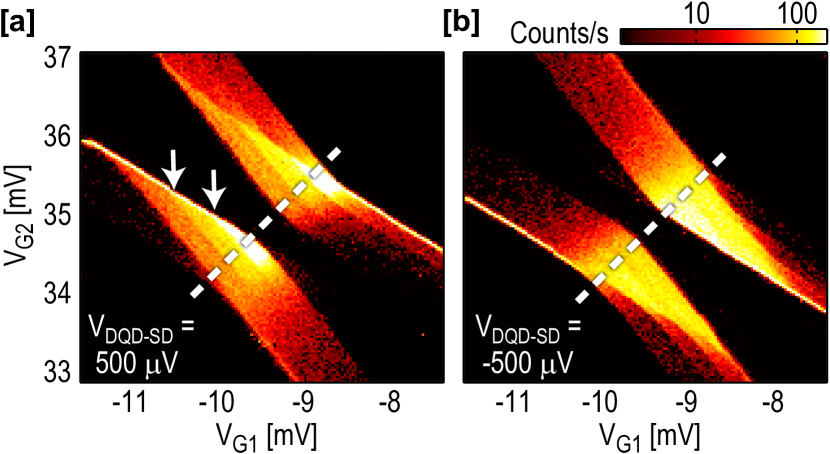
Figure 5: Finite-bias spectroscopy of the DQD, taken with positive (a) and negative (b) bias. The figures are constructed by counting electrons entering and leaving the DQD. Excited states are visible, especially for the positive bias data [marked with arrows in (a)]. The data was taken with $V_{\mathrm{DQD-SD}}=\pm 500\,\mu\mathrm{V}$, $V_{\mathrm{QPC-SD}}=250\,\mu\mathrm{V}$.

Figure 5 shows a magnification of two triangles from Fig. 1(b), measured with both negative and positive bias applied across the DQD. Excited states are visible within the triangles, especially for the case of positive bias [marked with arrows in Fig. 5(a)]. Transitions between excited states occur along parallel lines at which the potential of QD1 is held constant; this indicates that the excited states are located in QD1. To investigate the states more carefully, we measure the separate tunneling rates $\Gamma_{\mathrm{in}}$ and $\Gamma_{\mathrm{out}}$ along the dashed lines in Fig. 5. The results are presented in Fig. 6, together with a few sketches depicting the energy level configuration of the system.

We begin with the results for the positive bias case, which are plotted in Fig. 6(a). Going along the dashed line in Fig. 5(a) corresponds to keeping the detuning $\delta$ between the QDs fixed and shifting the total DQD energy. The measurements were performed with a small detuning ($\delta\approx 100\,\mu\mathrm{eV}$) to ensure that the electron transport is unidirectional. Because of this, the outermost parts of the traces in Fig. 6(a) correspond to regions where transport is due to cotunneling [compare the dashed line with the position of the triangle in Fig. 5(a)]; the regions where transport is sequential are shaded gray in Fig. 6(a).

Starting in the regime marked by I in Fig. 6(a,c), electrons may tunnel from source into the ground state of QD1, relax down to QD2 and tunnel out to the drain lead. Assuming the relaxation process to be much faster than the other processes, the measured rates $\Gamma_{\mathrm{in}}$ and $\Gamma_{\mathrm{out}}$ are related to the tunnel couplings of the source and drain $\Gamma_{\mathrm{in}}\approx\Gamma_{\mathrm{S}}$ and $\Gamma_{\mathrm{out}}=\Gamma_{\mathrm{D}}$. Going to higher gate voltages lowers the overall energy of both QDs. At the position marked by an arrow in Fig. 6(a), there is a sharp increase in the rate for tunneling into the DQD. We attribute this to the existence of an excited state in QD1; as shown in case II in Fig. 6(c), the electron tunneling from source into QD1 may enter either into the ground $\mathrm{(n+1,m)}$ or the excited state $\mathrm{(n+1^{*},m)}$, giving an increase in $\Gamma_{\mathrm{in}}$. When further lowering the DQD energy another excited state comes into the bias window and $\Gamma_{\mathrm{in}}$ increases even more [second arrow in Fig. 6(a)]. The rate for tunneling out of the DQD shows only minor variations within the region of interest. This supports the assumption that the excited states quickly relax and that the electron tunnels out of the DQD from the ground state of QD2

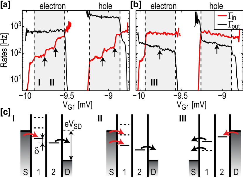
Figure 6: (a, b) Tunneling rates for electrons entering and leaving the DQD, measured along the dashed lines in Fig. 5(a, b). In (a), we show the results for positive bias across the DQD, in (b) the results for negative bias. The shaded areas mark the regions where electron transport is sequential, either in the electron or the hole transport cycle. The arrows indicate the positions of excited states. The data was extracted from QPC conductance traces of length $T=5\,\mathrm{s}$, taken with $\,\mathrm{V}_{\mathrm{QPC-SD}}=250\,\mathrm{mV}$. (c) Schematics of the DQD energy configuration at three different positions in (a, b).

Finally, continuing to the edge of the shaded region ($V_{\mathrm{G1}}\sim-9.55\,\mathrm{mV}$), the potential of QD2 goes below the Fermi level of the drain. Here, electrons get trapped in QD2 and the tunneling-out rate drops drastically. At the same time, $\Gamma_{\mathrm{in}}$ increases; when the electron in QD2 eventually tunnels out, the DQD may be refilled from either the source or the drain lead. The picture described above is repeated in the triangle with hole transport ($-9.25\,\mathrm{mV}<V_{\mathrm{G2}}<-8.9\,\mathrm{mV}$). This is expected, since the hole transport cycle involves the same QD states as in the electron case. An interesting feature is that $\Gamma_{\mathrm{in}}$ shows essentially the same values in both the electron and the hole cycle, while $\Gamma_{\mathrm{out}}$ increases by a factor of three. The presence of the additional electron in QD1 apparently affects the tunnel barrier between drain and QD2 more than an additional electron in QD2 affects the barrier between QD1 and source.

Next, we move over to the case of negative bias [Fig. 6(b)]. Here, the roles of QD1 and QD2 are inverted, meaning that electrons enter the DQD into QD2 and leave from QD1. Following the data and the arguments presented for the case of positive bias, one would expect this configuration to be suitable for detecting excited states in QD2. However, looking at the tunneling rates within the sequential region of Fig. 6(b), the rate for entering QD2 ($\Gamma_{\mathrm{in}}$) stays fairly constant, while the rate for tunneling out decreases at the point marked by the arrow. Again, we attribute the behavior to the existence of an excited state in QD1.

The situation is described in sketch III of Fig. 6(c). The electrochemical potential of QD1 is high enough to allow the electron in the $\mathrm{(n+1,m)}$-state to tunnel out to the source and leave the DQD in an excited state $\mathrm{(n^{*},m)}$. Since the energy difference $E[\mathrm{(n^{*},m)}]-E[\mathrm{(n+1,m)}]$ is smaller than $E[\mathrm{(n,m)}]-E[\mathrm{(n+1,m)}]$, the transition involving the excited state appears below the ground state transition. As the overall DQD potential is lowered, the transition energy involving the excited state goes below the Fermi level of the drain, resulting in a drop of $\Gamma_{\mathrm{out}}$ as only the ground state transition is left available. Similar to the single QD case Gustavsson et al. (2006b), the tunneling-in rate samples the excitation spectrum for the (n+1,m)-configuration, while the tunneling-out rate reflects the excitation spectrum of the $\mathrm{(n,m)}$-DQD.

To conclude the results of Fig. 6, we find two excited states in QD1 in the $\mathrm{(n+1,m)}$ configuration with $\Delta E_{1}^{\alpha}=180\,\mu\mathrm{eV}$ and $\Delta E_{1}^{\beta}=340\,\mu\mathrm{eV}$, and one excited state in QD1 in the $\mathrm{(n,m)}$ configuration, with $\Delta E_{1}=220\,\mu\mathrm{eV}$. No clear excited state is visible in QD2. This does not necessarily mean that such states do not exist; if they are weakly coupled to the lead they will only have a minor influence on the measured tunneling rates. Excited states in both QDs have been measured in other configurations; there, we find similar spectra of excited states for both QDs.

VI Inelastic cotunneling

Next, we investigate the cotunneling process in the presence of excited states. Looking carefully at the lower-right regions of the negative-bias triangles in Fig. 5(b), we see that the count rates in the cotunneling regions outside the triangles are not constant along lines of fixed detuning (corresponds to going in a direction parallel to the dashed line). Instead, the cotunneling regions seem to split into three parallel bands.

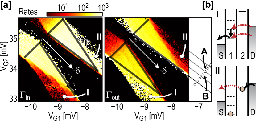
Figure 7: (a) Tunneling rates for electrons entering and leaving the DQD, extracted from the same set of data as used in Fig. 5(b). The data was measured with $V_{\mathrm{DQD-SD}}=-500\,\mu\mathrm{V}$. The solid lines mark the position of the finite-bias triangles. The plot region in the right-hand panel has been extended to include the regime investigated in Fig. 8. (b) Energy-level diagrams for the two positions marked in (a). In case I, the cotunneling itself is elastic, with energy relaxation occurring after the cotunneling has taken place. In case II, inelastic cotunneling processes are possible.

In Fig. 7(a), we plot the tunneling rates $\Gamma_{\mathrm{in}}$ and $\Gamma_{\mathrm{out}}$ for electrons entering and leaving the DQD, extracted from the same set of data as used in Fig. 5(b). The thick solid lines mark the edges of the finite-bias triangles. Again, the cotunneling rates outside the triangles are not uniform; parallel bands appear in $\Gamma_{\mathrm{in}}$ for the position marked by I and in $\Gamma_{\mathrm{out}}$ for the position marked by II in the figures.

To understand the data we draw energy level diagrams for the two configurations [see Fig. 7(b)]. Focusing first on case I, we see that the electrochemical potential of QD1 is within the bias window, whereas QD2 is detuned and in Coulomb blockade. The cotunneling occurs via QD2 states; electrons cotunnel from drain into QD1, followed by sequential tunneling from QD1 to the source lead. The picture is in agreement with what is measured in Fig. 7(a); the cotunneling rate ($\Gamma_{\mathrm{in}}$) is low and strongly depends on detuning $\delta$, while the sequential rate $\Gamma_{\mathrm{out}}$ is high and essentially independent of detuning. The three bands seen in $\Gamma_{\mathrm{in}}$ occur because of the excited states in QD1; depending on the average DQD energy, electrons may cotunnel from drain into one of the excited states, relax to the ground state and then leave to the source lead. The state of QD2 remains unaffected by the cotunneling process. For this configuration, we speak of elastic cotunneling.

The situation is different in case II. Here, cotunneling occurs in QD1 as electrons tunnel directly from QD2 into the source lead. This means that $\Gamma_{\mathrm{in}}$ is sequential while $\Gamma_{\mathrm{out}}$ describe the cotunneling process. As in case I, the cotunneling rate $\Gamma_{\mathrm{out}}$ splits up into three bands; we attribute this to cotunneling where the state of QD1 is changed during the process. QD1 ends up in one of its excited states. The energy of the electron arriving in the source lead is correspondingly decreased compared to the electrochemical potential of QD2. Here, the cotunneling is inelastic.

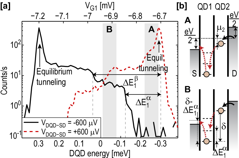
Figure 8: (a) Electron count rate along the dashed line in Fig. 7(a), measured for both positive and negative DQD bias. In the trace, the detuning $\delta$ stays constant and we sweep the average DQD energy. The DQD energy is defined from the position where the electrochemical potential of QD2 is right in the middle between the Fermi levels of the source and drain leads [see the dotted line in the energy level diagram in (b)]. The steps in the count rate are due to the onset of inelastic cotunneling processes in QD1. The data was extracted from traces of length $T=10\,\mathrm{s}$, measured with $V_{\mathrm{QPC-SD}}=200\,\mu\mathrm{V}$. (b) Energy level diagrams for the two configurations marked in (a).

The inelastic cotunneling is described in greater detail in Fig. 8. In Fig. 8(a) we plot the count rate for positive and negative DQD bias, measured along the dashed line at the right edge of Fig. 7(a). Figure 8(b) shows energy level diagrams for negative bias at two positions along this line. The bias voltage is applied symmetrically to the DQD, meaning that the Fermi levels in source and drain leads are shifted by $\pm eV/2$ relative to the Fermi energy at zero bias [dotted line in Fig. 8(b)]. In the measurement of Fig. 8(a) we sweep the average DQD energy while keeping the detuning $\delta$ constant. The average DQD energy is defined to be zero when $\mu_{2}$ aligns with the zero-bias Fermi energy in the leads [i.e. when $\mu_{2}=(\mu_{\mathrm{S}}+\mu_{\mathrm{D}})/2$].

Starting in the configuration marked by A, cotunneling is only possible involving the QD2 ground state. Cotunneling is weak, with count rates being well below 1 count/s. Continuing to case B, we raise the average DQD energy. When the electrochemical potential of QD2 is sufficiently increased compared to the Fermi level of the source, inelastic cotunneling becomes possible leading to a sharp increase in count rate. The process is sketched in Fig. 8(b); it involves the simultaneous tunneling of an electron from QD2 to the first excited state of QD1 with an electron in the QD1 ground state leaving to the source. The process is only possible if

$$\delta-\Delta E^{\alpha}_{1}=\mu_{1}-\mu_{2}-\Delta E^{\alpha}_{1}>\mu_{\mathrm{S}}-\mu_{1}.$$ (7)

Here, $\Delta E^{\alpha}_{1}$ is the energy of the first excited state in QD1. The position of the step in Fig. 8(a) directly gives the energy of the first excited state, and we find $\Delta E^{\alpha}_{1}=180\,\mu\mathrm{eV}$.

Further increasing the average DQD energy makes an inelastic process involving the second excited state in QD2 possible, giving $\Delta E^{\alpha}_{2}=340\,\mu\mathrm{eV}$. Finally, as the DQD energy is raised to become equal to half the applied bias, the electrochemical potential of QD2 aligns with Fermi level of the drain lead. Here electron tunneling mainly occurs due to equilibrium fluctuations between drain and QD2, giving a sharp peak in the count rate. The excited states energies extracted from the inelastic cotunneling give the same values as obtained from finite-bias spectroscopy within the triangles, as described in the previous section. The good agreement between the two measurements demonstrates the consistency of the model.

The dashed line in Fig. 8(a) shows data taken with reversed DQD bias; for this configuration the Fermi levels of the source and drain leads are inverted, the electrons cotunnel from source to QD2 and the peak due to equilibrium tunneling occurs at $\mu_{2}=\mu_{\mathrm{D}}=-300\,\mu\mathrm{eV}$.

VII Noise in the cotunneling regime

Using time-resolved charge detection methods, we can extract the noise of electron transport in the cotunneling regime. For a weakly-coupled single QD in the regime of sequential tunneling, transport in most configurations is well-described by independent tunneling events for electrons entering and leaving the QD Gustavsson et al. (2006a). The Fano factor becomes a function of the tunneling rates Davies et al. (1992):

$$F_{2}=\frac{S_{I}}{2eI}=\frac{\Gamma_{\mathrm{in}}^{2}+\Gamma_{\mathrm{out}}^{2}}{(\Gamma_{\mathrm{in}}+\Gamma_{\mathrm{out}})^{2}}=\frac{1}{2}\left(1+a^{2}\right),$$ (8)

with $a=(\Gamma_{\mathrm{in}}-\Gamma_{\mathrm{out}})/(\Gamma_{\mathrm{in}}+\Gamma_{\mathrm{out}})$. For symmetric barriers ($a=0$), the Fano factor is reduced to 0.5 because of an increase in electron correlation due to Coulomb blockade. In the case of cotunneling, the situation is more complex. As described in the previous section, cotunneling may involve processes leaving either QD in an excited state. The excited state has a finite lifetime $\tau_{\mathrm{rel}}$; during this time, the tunneling rates may be different compared to the ground-state configuration Schleser et al. (2005). We therefore expect that the existence of an electron in an excited state may induce temporal correlations on time scales on the order of $\tau_{\mathrm{rel}}$ between subsequent cotunneling events. In this way, the noise of the cotunneling current has been proposed as a tool to probe excited states and relaxation processes in QDs Aghassi et al. (2006, 2008).

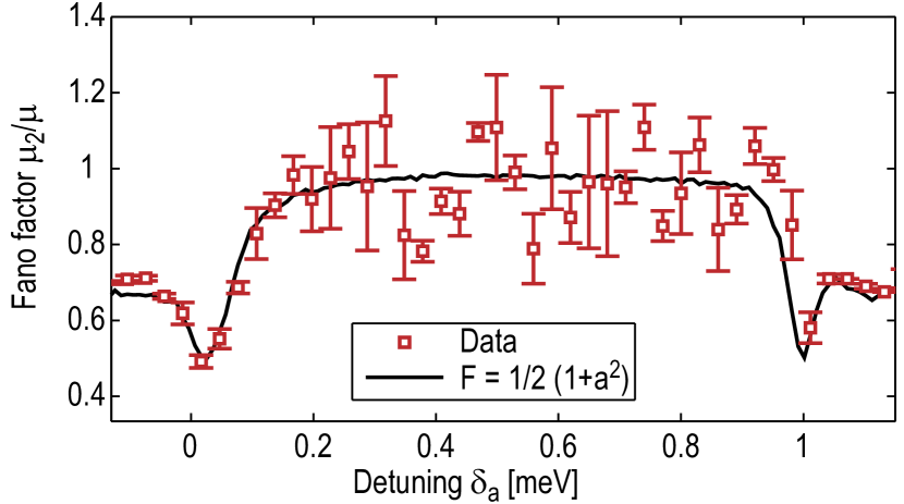
Figure 9: Fano factor for electron transport in the cotunneling regime of Fig. 3. The data was extracted from traces of length $T=30\,\mathrm{s}$. The solid line is the result of Eq. (8), which assumes independent tunneling events. The minima in Fano factor occur at positions where the tunneling rates $\Gamma_{\mathrm{in}}$ and $\Gamma_{\mathrm{out}}$ are equal (see Fig. 3). The error bars show standard error, extracted by splitting the data into six subsets of length $T=5\,\mathrm{s}$ and evaluating the noise for each subset.

In Fig. 9, we plot the Fano factor measured from the same region as that of Fig. 3. The Fano factor was extracted by measuring the distribution function for transmitted charge through the system Gustavsson et al. (2006a). The solid line shows the result of Eq. (8), with tunneling rates extracted from the measured traces. In the outermost regions of the graph, the electrons tunnel sequentially through the DQD. Here, the Fano factor is reduced due to Coulomb blockade, similar to the single QD case. At the edges of the cotunneling regions, the Fano factor drops further down to $F=0.5$. This is because the injection rate $\Gamma_{\mathrm{in}}$ drops drastically as sequential transport becomes unavailable, while $\Gamma_{\mathrm{out}}$ stays approximately constant. At some point we get $\Gamma_{\mathrm{in}}=\Gamma_{\mathrm{out}}$, which means that the asymmetry $a$ is zero and the Fano factor of Eq. (8) shows a minimum. Further into the cotunneling region, the Fano factor approaches one as transport essentially becomes limited by a single rate; the cotunneling rate ($\Gamma_{\mathrm{in}}$) is two orders of magnitude smaller than the sequential rate $\Gamma_{\mathrm{out}}$.

We do not see any major deviation from the results of Eq. (8), which is only valid assuming independent tunneling events. We have performed similar measurements in several inelastic and elastic cotunneling regimes, without detecting any clear deviations from Eq. (8). As it turns out, there are two effects that make it hard to detect correlations due to the internal QD relaxations. For the first, the correlation time is essentially set by the relaxation time $\tau_{\mathrm{rel}}$, which typically occurs on a $\sim\!10~{}\mathrm{ns}$ timescale. This is several orders of magnitude smaller than a typical tunneling time of $\sim 1/\Gamma_{\mathrm{in}}\sim 100\,\mathrm{ms}$ Fujisawa et al. (2002). Secondly, the slow cotunneling rate limits the amount of experimental data available within a reasonable measurement time. This explains the large spread between the data points in Fig. 9 in the cotunneling regime. We conclude that the measurement bandwidth currently limits the possibility of examining correlations in the cotunneling regime using time-resolved detection techniques. A higher-bandwidth detector would solve both the above mentioned problems. It would allow a general increase of the tunneling rates in the system, which would both decrease the difference between $\tau_{\mathrm{cot}}$ and $\tau_{\mathrm{rel}}$ as well as provide faster acquisition of sufficient statistics.

To conclude, we have used time-resolved charge-detection techniques to investigate tunneling of single electrons involving virtual processes. The measurement method provides precise determination of all coupling energies, which allows a direct comparison with tunneling rates expected from time-energy uncertainty. The results give experimental confirmation of the equivalence between cotunneling through atomic states and sequential tunneling into molecular states. In the high-bias regime, we measure inelastic cotunneling due to virtual processes involving excited states of the double quantum dot. For future experiments with a high-bandwidth detector, the method may provide a way to probe relaxation processes and internal charge dynamics in quantum dots.

References

- van der Wiel et al. (2002) W. G. van der Wiel, S. De Franceschi, J. M. Elzerman, T. Fujisawa, S. Tarucha, and L. P. Kouwenhoven, Rev. Mod. Phys. 75, 1 (2002).
- Hayashi et al. (2003) T. Hayashi, T. Fujisawa, H. D. Cheong, Y. H. Jeong, and Y. Hirayama, Phys. Rev. Lett. 91, 226804 (2003).
- Petta et al. (2004) J. R. Petta, A. C. Johnson, C. M. Marcus, M. P. Hanson, and A. C. Gossard, Phys. Rev. Lett. 93, 186802 (2004).
- Golovach and Loss (2004) V. N. Golovach and D. Loss, Phys. Rev. B 69, 245327 (2004).
- Averin and Nazarov (1990) D. V. Averin and Y. V. Nazarov, Phys. Rev. Lett. 65, 2446 (1990).
- De Franceschi et al. (2001) S. De Franceschi, S. Sasaki, J. M. Elzerman, W. G. van der Wiel, S. Tarucha, and L. P. Kouwenhoven, Phys. Rev. Lett. 86, 878 (2001).
- Zumbühl et al. (2004) D. M. Zumbühl, C. M. Marcus, M. P. Hanson, and A. C. Gossard, Phys. Rev. Lett. 93, 256801 (2004).
- Schleser et al. (2005) R. Schleser, T. Ihn, E. Ruh, K. Ensslin, M. Tews, D. Pfannkuche, D. C. Driscoll, and A. C. Gossard, Phys. Rev. Lett. 94, 206805 (2005).
- Liu et al. (2005) H. W. Liu, T. Fujisawa, T. Hayashi, and Y. Hirayama, Phys. Rev. B 72, 161305 (2005).
- Field et al. (1993) M. Field, C. G. Smith, M. Pepper, D. A. Ritchie, J. E. F. Frost, G. A. C. Jones, and D. G. Hasko, Phys. Rev. Lett. 70, 1311 (1993).
- Fujisawa et al. (2004) T. Fujisawa, T. Hayashi, Y. Hirayama, H. D. Cheong, and Y. H. Jeong, Appl. Phys. Lett. 84, 2343 (2004).
- Schleser et al. (2004) R. Schleser, E. Ruh, T. Ihn, K. Ensslin, D. C. Driscoll, and A. C. Gossard, Appl. Phys. Lett. 85, 2005 (2004).
- Vandersypen et al. (2004) L. M. K. Vandersypen, J. M. Elzerman, R. N. Schouten, L. H. Willems van Beveren, R. Hanson, and L. P. Kouwenhoven, Appl. Phys. Lett. 85, 4394 (2004).
- Elzerman et al. (2004) J. M. Elzerman, R. Hanson, L. H. Willems van Beveren, B. Witkamp, L. M. K. Vandersypen, and L. P. Kouwenhoven, Nature 430, 431 (2004).
- Gustavsson et al. (2008a) S. Gustavsson, R. Leturcq, M. Studer, T. Ihn, K. Ensslin, D. C. Driscoll, and A. C. Gossard, Nano Letters 8, 2547 (2008a).
- Gustavsson et al. (2006a) S. Gustavsson, R. Leturcq, B. Simovic, R. Schleser, T. Ihn, P. Studerus, K. Ensslin, D. C. Driscoll, and A. C. Gossard, Phys. Rev. Lett. 96, 076605 (2006a).
- Fujisawa et al. (2006) T. Fujisawa, T. Hayashi, R. Tomita, and Y. Hirayama, Science 312, 1634 (2006).
- Gustavsson et al. (2008b) S. Gustavsson, I. Shorubalko, R. Leturcq, S. Schön, and K. Ensslin, Appl. Phys. Lett. 92, 152101 (2008b).
- Fuhrer et al. (2002) A. Fuhrer, A. Dorn, S. Lüscher, T. Heinzel, K. Ensslin, W. Wegscheider, and M. Bichler, Superl. and Microstruc. 31, 19 (2002).
- Gustavsson et al. (2007) S. Gustavsson, M. Studer, R. Leturcq, T. Ihn, K. Ensslin, D. C. Driscoll, and A. C. Gossard, Phys. Rev. Lett. 99, 206804 (2007).
- Naaman and Aumentado (2006) O. Naaman and J. Aumentado, Phys. Rev. Lett. 96, 100201 (2006).
- DiCarlo et al. (2004) L. DiCarlo, H. J. Lynch, A. C. Johnson, L. I. Childress, K. Crockett, C. M. Marcus, M. P. Hanson, and A. C. Gossard, Phys. Rev. Lett. 92, 226801 (2004).
- Gustavsson et al. (2006b) S. Gustavsson, R. Leturcq, B. Simovic, R. Schleser, P. Studerus, T. Ihn, K. Ensslin, D. C. Driscoll, and A. C. Gossard, Phys. Rev. B 74, 195305 (2006b).
- Kouwenhoven et al. (1997) L. P. Kouwenhoven, C. M. Marcus, P. M. McEuen, S. Tarucha, R. M. Westervelt, and N. S. Wingreen, in Mesoscopic Electron Transport, edited by L. L. Sohn, L. P. Kouwenhoven, and G. Schön (Kluwer, Dordrecht, 1997), NATO ASI Ser. E 345, pp. 105–214.
- Averin and Nazarov (1992) D. V. Averin and Y. V. Nazarov, Single Charge Tunneling (Plenum, New York, 1992).
- MacLean et al. (2007) K. MacLean, S. Amasha, I. P. Radu, D. M. Zumbühl, M. A. Kastner, M. P. Hanson, and A. C. Gossard, Phys. Rev. Lett. 98, 036802 (2007).
- Pohjola et al. (1997) T. Pohjola, J. Konig, M. M. Salomaa, J. Schmid, H. Schoeller, and G. Schon, Europhysics Letters 40, 189 (1997).
- Gräber et al. (2006) M. R. Gräber, W. A. Coish, C. Hoffmann, M. Weiss, J. Furer, S. Oberholzer, D. Loss, and C. Schönenberger, Phys. Rev. B 74, 075427 (2006).
- Pedersen et al. (2007) J. N. Pedersen, B. Lassen, A. Wacker, and M. H. Hettler, Phys. Rev. B 75, 235314 (2007).
- Davies et al. (1992) J. H. Davies, P. Hyldgaard, S. Hershfield, and J. W. Wilkins, Phys. Rev. B 46, 9620 (1992).
- Aghassi et al. (2006) J. Aghassi, A. Thielmann, M. H. Hettler, and G. Schön, Phys. Rev. B 73, 195323 (2006).
- Aghassi et al. (2008) J. Aghassi, M. H. Hettler, and G. Schon, App. Phys. Lett. 92, 202101 (2008).
- Fujisawa et al. (2002) T. Fujisawa, D. G. Austing, Y. Tokura, Y. Hirayama, and S. Tarucha, Nature 419, 278 (2002).