Impact of impellers on the axisymmetric magnetic mode in the VKS2 dynamo experiment

Abstract

In the VKS2 (von Kármán Sodium 2) successful dynamo experiment of September 2006, the magnetic field that was observed showed a strong axisymmetric component, implying that non axisymmetric components of the flow field were acting. By modeling the induction effect of the spiraling flow between the blades of the impellers in a kinematic dynamo code, we find that the axisymmetric magnetic mode is excited and becomes dominant in the vicinity of the dynamo threshold. The control parameters are the magnetic Reynolds number of the mean flow, the coefficient measuring the induction effect, $\alpha$, and the type of boundary conditions (vacuum for steel impellers and normal field for soft iron impellers). We show that using realistic values of $\alpha$, the observed critical magnetic Reynolds number, $Rm^{c}\approx 32$, can be reached easily with ferromagnetic boundary conditions. We conjecture that the dynamo action achieved in this experiment may not be related to the turbulence in the bulk of the flow, but rather to the alpha effect induced by the impellers.

The interest of the scientific community for the dynamo action in liquid metal has been renewed since 2000 in the wake of successful experiments Ga2000 ; StMu01 ; Monchaux06 . We focus in this Letter on the Cadarache VKS2 (von Kármán Sodium 2) experiment Monchaux06 where the dynamo effect occurred beyond the critical magnetic Reynolds number $Rm^{c}\approx 32$. The growing magnetic field that was observed above threshold was mainly axisymmetric. Dynamo action was found with soft iron impellers but did not occur with stainless steel impellers, using the same available power. The purpose of the present Letter is to present arguments based on modeling and numerical simulations to justify the observed axisymmetric mode. The two key ingredients are the so-called $\alpha$-effect and ferromagnetic boundary conditions.

From Cowling’s theorem Cowling34 the axisymmetric part of the flow cannot be responsible alone for the generation of an axisymmetric field. In the experiment, the deviation from axisymmetry of the velocity field is thus expected to participate to the dynamo process, generating an axisymmetric electromotive force somewhere in the fluid and triggering the dynamo growth. Two other magnetohydrodynamic experiments using counter-rotating propellers have also led to this conclusion either on observational Lathrop00 ; Forest06 or on numerical grounds Forest07 . It was argued in Lathrop00 ; Forest06 ; Forest07 that turbulence effects were responsible for the occurrence of the axisymmetric magnetic field. In Petrelis07 the turbulence effects were held responsible for the dynamo threshold in VKS2. In addition an $\alpha$-effect close to the discs was invoked to justify the axisymmetry of the generated field.

The VKS2 configuration is modeled as follows: The computational domain is divided into three concentric cylinders of axis $z$, embedded in an insulating sphere (figure 1). The inner cylinder $r\leq R_{0}$ contains the moving sodium of conductivity $\sigma_{0}$. The cylindrical shell $R_{0}\leq r\leq R_{1}$ contains stagnant sodium ($\sigma_{1}=\sigma_{0}$). The cylindrical shell $R_{1}\leq r\leq R_{2}$ is a layer of copper ($\sigma_{2}=4.5\sigma_{0}$). We choose $R_{0}$ as unit length and the geometric parameters are $R_{1}/R_{0}=1.4$, $R_{2}/R_{0}=1.6$ and $R_{out}/R_{0}=10$, with the same height $H/R_{0}=1.8$ for the three cylinders. The velocity field of the liquid sodium U ($r<R_{0}$) is axisymmetric and is obtained from time averaged measurements of a water experiment in the VKS2 setting Ravelet05 . The meridional flow field and the isolines of the azimuthal component of the velocity are shown in figure 1.

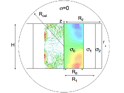
Figure 1: Geometry of the computational domain in a meridional plane. The axisymmetric meridional flow $(U_{r},U_{z})$ is represented on the left with arrows. On the right the isovalues of $U_{\theta}$ are plotted. The radii $R_{i}$ and height $H$ as well as the conductivities $\sigma_{i}$ are defined in the text.

The flow field is maintained by two counter-rotating impellers located at both ends of the vessel. They each occupy a cylindrical volume of radius $R_{0}$ and thickness $H/20$.

The only non axisymmetric parts of the device are the blades composing the impellers (eight each), and we represent the effect of these blades by adding the electromotive force $\alpha(\textbf{B}\cdot\textbf{e}_{\theta})\textbf{e}_{\theta}$ to the induction equation. This force is assumed to act only in the two fluid cylinders occupied by the blades as they rotate. This model is deduced as follows: As the blades rotate, the fluid is ejected radially outwards and radial vortices are created due to the rotation rate gradient, see the white arrows in figure 2. We then assume that when a magnetic field is applied, the mean induced current is dominated by its azimuthal component and that the shearing action of the vortices is cumulative. The axial current is expected to vanish in the vicinity of the discs and, as a result, we set the $\alpha_{zz}$ component of the $\alpha$ tensor to be zero. This phenomenon is illustrated on fig. 2. As the magnetic lines $(\textbf{B}\cdot\textbf{e}_{\theta})\textbf{e}_{\theta}$ (thin line in figure 2) are distorted by the helical vortices, small scale magnetic loops are created, which in turn create an azimuthal electromotive force $\alpha(\textbf{B}\cdot\textbf{e}_{\theta})\textbf{e}_{\theta}$, where the parameter $\alpha$ is negative and depends on the impeller rotation rate (see below for an estimate), the size, curvature and number of blades. We thus attempt to represent the complexity of the induction effects in a poorly known flow close to a boundary by a single scalar parameter. The handedness of the helical vortices generated between the blades is directly linked to the rotation sign of the impellers: orienting the rotation axis of the bottom impeller towards the center of the container, a positive rotation drives a set of eight radial positive helices creating a negative $\alpha$ coefficient. The counter-rotation configuration with $\Omega_{\text{bot}}=-\Omega_{\text{top}}$ is invariant by rotation of $\pi$ about any horizontal axis NTDX03 , therefore the two impellers produce the same $\alpha$. Actually, whatever the sign for the rotation of the bottom impeller, $\Omega$, the product $\Omega\alpha$ is always negative. Henceforth we set $\Omega_{\text{bot}}=\Omega>0$.

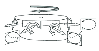
Figure 2: Sketch of the top impeller with eight radial blades attached to the disc. Due to the rotation of the disc (gray arrow on the top), radial helical vortices are produced between the blades (thick white arrows). An axisymmetric azimuthal field $(\textbf{B}\cdot\textbf{e}_{\theta})\textbf{e}_{\theta}$ (thin line) is distorted leading to eight magnetic loops.

We follow the standard kinematic dynamo approach by solving the induction equation

$$\partial_{t}\textbf{B}=\nabla\times(\widetilde{\textbf{U}}\times\textbf{B}+\alpha(\textbf{B}\cdot\textbf{e}_{\theta})\textbf{e}_{\theta})-\nabla{\times}(\eta\nabla{\times}\textbf{B}).$$ (1)

where $\eta=1/\sigma\mu_{0}$, $\mu_{0}$ being the vacuum magnetic permeability, $\sigma$ the fluid conductivity and $\alpha$ the unknown parameter which models the induction effect in the volume occupied in average by the impellers. The field $\widetilde{\textbf{U}}$ is equal to U in the cylinder $r\leq R_{0}$ and is zero in the two cylindrical shells $R_{0}\leq r\leq R_{1}$, $R_{1}\leq r\leq R_{2}$. The conductivity field is such that $\sigma=\sigma_{0}$ in the inner cylinder $r\leq R_{0}$ and in the stagnant sodium shell, and $\sigma=\sigma_{2}$ in the copper layer. The conductivity jump at $r=R_{1}$ is accounted for by enforcing the continuity of the tangent component of the electric field. Note that the flow behind the impellers has not been simulated (see discussion below). To simplify the parameterization of the alpha effect, $\alpha$ vanishes outside two thin cylindrical layers of radius $R_{0}$ and thickness $H/20$ situated at each end of the container and its intensity varies smoothly within these layers using a $\tanh$ regularization function. The magnetic Reynolds number is $Rm\equiv\sigma_{0}\mu_{0}U_{0}R_{0}$ where $U_{0}$ is the maximum speed of the flow U.

Two types of boundary conditions are compared to model the experiment: they are referred to as insulating (I) and ferromagnetic (F) boundary conditions. We say that insulating boundary conditions (I) are used when the continuity of the magnetic field is enforced at the interface between the conducting regions and the vacuum (i.e., at ${|z|=H/2,\,0\leq r\leq R_{2}}$ and at ${0\leq|z|\leq H/2,\,r=R_{2}}$). We say that ferromagnetic boundary conditions (F) are used when we enforce $\textbf{B}\times\textbf{e}_{z}=0$ at ${|z|=H/2,\,0\leq r\leq R_{0}}$ and we require B to be continuous across the other boundaries ${0\leq|z|\leq H/2,\,r=R_{2}}$ and ${|z|=H/2,\,R_{0}\leq r\leq R_{2}}$. The condition $\textbf{B}\times\textbf{e}_{z}=0$ is meant to mimic the effect of ferromagnetic discs with infinite magnetic permeability located at the top and bottom of the vessel Durand68 . These boundary conditions model steel impellers (I) and soft iron impellers (F), respectively.

Our numerical code Laguerre06 ; Guermond07 uses a finite element Galerkin method for the spatial discretization in the meridional plane $(r,z)$ and a Fourier series decomposition along the azimuthal direction. Since the coefficients of the induction equation do not depend on the azimuthal angle, the different azimuthal modes ($m=0,1,2,\ldots$) are decoupled. The time is discretized with a semi-implicit backward finite difference method of second order. Growth rates are computed for the two types of magnetic boundary conditions, (I) or (F), and for various values of $\alpha$ and $Rm$. The zero growth rate condition defines a critical curve in the ($\alpha$, $Rm$) plane. A compilation of results obtained for the (I) and (F) cases and for Fourier modes $m=0$ and $m=1$ is shown in figure 3.

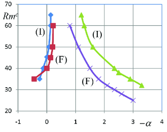
Figure 3: Dynamo threshold $Rm^{c}$ versus $-\alpha$, for ($\times$, $\triangle$) $m=0$, ($\square$,$\diamond$) $m=1$ and where (F) and (I) indicate ferromagnetic and insulating boundary conditions respectively.

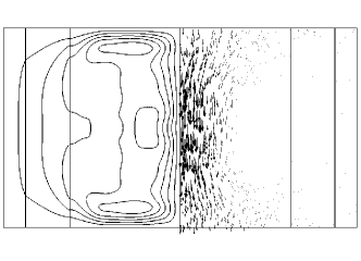
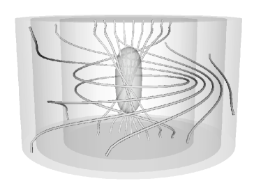
Figure 4: Top: Geometry of the $m=0$ (F) growing magnetic field for $Rm^{c}=32$, $|\alpha|=2.2>|\alpha_{c}|=2.1$ . The three cylinders are also represented. The lines correspond to the positive isovalues of $B_{\theta}$ and the arrows to the meridional field $(B_{r},B_{z})$. Bottom: isovalue of 25% of the maximum energy plotted in the 3D domain, together with some field lines.

In order to make comparisons with experimental results published in Monchaux06 , we first focus our attention on the axisymmetric magnetic mode ($m=0$), which was a priori eliminated in former studies by Cowling’s theorem. The two critical curves corresponding to the boundary conditions (I) and (F) and the Fourier mode $m=0$ reveal that the dynamo action occurs only for $\alpha$ negative, thus confirming the phenomenological argument discussed above to justify the sign of $\alpha$. Both curves clearly show that increasing $|\alpha|$ lowers the critical magnetic Reynolds number. Moreover, the (F) boundary condition yields significantly smaller thresholds. This observation agrees with previous results obtained in a different context Avalos03 ; Avalos05 . Both curves can be represented by the scaling law $Rm^{c}\sim|\alpha|^{-q}$, where $q\approx 0.67$, suggesting that the dynamo process is similar for both types of boundary conditions.

The value of $\alpha$ corresponding to the dynamo threshold in VKS2, $Rm^{c}=32$, is found to be $|\alpha|=2.1$ for the (F) boundary condition and $|\alpha|=3.3$ for the (I) boundary condition. Since the steel impellers have not produced dynamo action, this suggests that, as a first guess, the effective $|\alpha|$ for VKS2 is between 2.1 and 3.3. A rough estimate of $\alpha$ is given by $\alpha\sim u^{2}h/\eta$ where $u$ is a typical flow intensity between the blades and $h=H/20$. From Ravelet05 we estimate $u/U_{0}\sim 0.2$ at the impeller half radius. Then, for $Rm=32$, $\eta$=0.1 m².s^-1 and $R_{0}=0.2$m, we find $\alpha\sim 1.8$m.s^-1, making the value $|\alpha|$ = 2.1m.s^-1 plausible. If $|\alpha|$ is indeed close to 2.1, the critical value of $Rm$ for the (I) boundary condition is close to 43, which apparently contradicts the experiments since $Rm=50$ has been reached without dynamo action using steel impellers. To explain this discrepancy we recall that it has been shown in Stefani06 that for the Fourier mode $m=1$ the flow of liquid sodium behind the impellers acts against the dynamo action. We expect this anti-dynamo effect to be active also for the Fourier mode $m=0$, but we did not include this extra layer of fluid in the present study. The negative consequences of this secondary flow are probably screened in the case of soft iron impellers. The numerical evidence justifying this assertion has to await the availability of a code describing conducting domains with different magnetic permeabilities (work in progress).

The stationary eigenvector corresponding to the (F) boundary condition for $m=0$ and $|\alpha|=2.2$ is shown in figure 4. The magnetic field is mainly concentrated along the $z$-axis in the fluid region $r\leq R_{0}$, and it is azimuthally dominated in the plane $z=0$ for $r\geq R_{0}$. The radial component is odd with respect to $z$ whereas the azimuthal and vertical components are even and of opposite sign. These features are compatible with the magnetic field measured at saturation in the experimental dynamo regime obtained with soft iron impellers Monchaux06 . The eigenvector corresponding to the (I) boundary condition for $m=0$ and $|\alpha|=2.2$ (not shown here) is associated to an eigenvalue with a nonzero imaginary part. The resulting dynamo is periodic with a reversing dipolar moment. This result, not detailed here, is in strong contrast with the case $\alpha=0$ (I), for which a non oscillatory transverse dipole mode ($m=1$) with internal banana-like structures is the only unstable mode Ravelet05 .

We have also investigated the effect of the $\alpha$ model on the Fourier mode $m=1$. This mode has not been observed in the VKS2 experiment although it has been predicted to be the most unstable in axisymmetric kinematic dynamo simulations Ravelet05 ; Marie06 ; Stefani06 ; Laguerre_thesis . In figure 3, for the mode $m=1$, we see that the critical magnetic Reynolds number grows sharply with $|\alpha|$ for $\alpha<0$ and decreases with $|\alpha|$ for $\alpha>0$. We are thus led to conclude that the growth of the $m=1$ mode is hindered by the very induction effect that generates the $m=0$ mode! This surprising result may explain the absence of the $m=1$ mode in the experiment, at least for $Rm<50$.

The present study shows that the positive results of the dynamo experiment of September 2006 (VKS2) as well as the former negative results (VKS1) may be explained by a simple mean induction effect induced by the radial vortices trapped between the blades of the impellers. We conjecture that turbulence may not play a role as essential as initially believed in the VKS experiments.

This work also shows the importance of using ferromagnetic materials, corresponding to the (F) boundary conditions in fig. 3. A research program aiming at exploring the saturation regime using nonlinear computations and materials with heterogeneous magnetic permeabilities is currently engaged.

This work was supported by ANR project no. 06-BLAN-0363-01 “HiSpeedPIV”. We are pleased to acknowledge the Saclay VKS-team for providing us with a mean velocity field measured in a water experiment. We acknowledge fruitful discussions with F. Stefani. We warmly thank D. Carati and B. Knaepen, the organizers of the MHD Summer Program, Bruxelles, July 2007. The computations were carried out on the IBM Power 4 computer of IDRIS of CNRS (project # 0254).

References

- (1) A. Gailitis, O. Lielausis, S. Dement’ev, E. Platacis and A. Cifersons, Phys. Rev. Lett., 84, 4365 (2000).
- (2) R. Stieglitz and U. Müller, Phys. Fluids, 13, 561 (2001).
- (3) R. Monchaux et al., Phys. Rev. Lett. 98, 044502 (2007).
- (4) T.G. Cowling, Mon. Not. Roy. Astr. Soc. 94, 39-48 (1934).
- (5) N. Peffley, A. Cawthorne and D. Lathrop, Phys. Rev. E, 61, 5287 (2000).
- (6) E. J. Spence, C. B. Forest, M. D. Nornberg and R. D. Kendrick, Phys. Rev. Lett. 96, 055002 (2006).
- (7) R. A. Bayliss, C. B. Forest, M. D. Nornberg, E. J. Spence and P. W. Terry, Phys. Rev. E 75:2, 026303 (2007).
- (8) F. Pétrélis, N. Mordant and S. Fauve, Geophys. Astrophys. Fluid Dyn. 101, 289 (2007).
- (9) F. Ravelet, A. Chiffaudel, F. Daviaud and J. Léorat, Phys. Fluids 17, 117104 (2005).
- (10) C. Nore, L. S. Tuckerman, O. Daube and S. Xin, J. Fluid Mech., 477, 51-88 (2003).
- (11) E. Durand, Magnétostatique, Masson (1968).
- (12) R. Laguerre, C. Nore, J. Léorat and J. L. Guermond, CR Mécanique 334, 593 (2006).
- (13) J. L. Guermond, R. Laguerre, J. Léorat and C. Nore, J. Comp. Physics 221, 349 (2007).
- (14) R. Avalos-Zuñiga, F. Plunian and A. Gailitis, Phys. Rev. E 68, 066307 (2003).
- (15) R. Avalos-Zuñiga and F. Plunian, Eur. Phys. J. B 47, 127 (2005).
- (16) F. Stefani et al., Eur. J. Mech. B/Fluids 25 894 (2006).
- (17) L. Marié, C. Normand and F. Daviaud, Phys. Fluids 18, 017102 (2006).
- (18) R. Laguerre, PhD thesis, Université Paris VII (2006).