Contribution of final state interaction to the branching ratio of $B\to J/\psi D$

Abstract

To testify the validity of the perturbative QCD (pQCD) and investigate its application range, one should look for a suitable process to do the job. $B\to J/\psi D$ is a promising candidate. The linear momentum of the products is relatively small, so that there may exist a region where exchanged gluons are soft and the perturbative treatment may fail, so that the non-perturbative effect would be significant. We attribute such non-perturbative QCD effects into the long-distance final state interaction (FSI) which is estimated in this work. We find that the contribution from the FSI to the branching ratio is indeed sizable and may span a rather wide range of $10^{-6}\sim 10^{-5}$, and cover a region where the pQCD prediction has the same order. A more accurate measurement on its branching ratio may provide important information about the application region of pQCD and help to clarify the picture of the inelastic rescattering (i.e. FSI) which is generally believed to play an important role in $B$ decays.

I introduction

It is well known that $B$ physics may provide an ideal field for testing all the existing theoretical frameworks, methods and searching new physics beyond the standard model (SM). The reason is that because there exists a heavy flavor, some approximations, such as the $1/M_{Q}$ expansion can be adopted, so that the results of perturbative calculations are more reliable. When the study gets deeper, defects of such theoretical frameworks have been unavoidably exposed and demand further improving the standing theories. The most fundamental problem is how to properly evaluate the hadronic matrix elements which are fully governed by non-perturbative QCD. Thanks to the factorization, one can separate the non-perturbative QCD effects from the perturbative parts and the later one is calculable in terms of the field theory order by order. Based on this picture, various theories, such as the naive QCD factorization, pQCD (perturbative QCD) and the soft-collinear-effective theory (SCET) etc. are invented to calculate the processes where $B$ mesons are involved.

The pQCD has been proved to be a successful approach in $B$ physics, namely most of the results obtained in this approach are consistent with data of the Babar, Belle and CLEO experiments. In this approach, the infrared divergence is properly dealt with by taking into account the contribution of the transverse momentum of quarks $k_{T}$. In this picture, the non-perturbative part is included in the wavefunctions of the initial $B$ meson and the produced hadrons. Obviously, as one factorizes the perturbative part out and calculates the quark-level transition amplitudes, he must assume that all the constituents which participate in the reaction are not far from their mass shells and moreover, all the internal lines (no matter quark line or gluon line) must be hard enough, so that the perturbative calculation can make sense. A natural question would be raised, whether the pQCD framework is complete, even though its validity is supposed to be respected. By the asymptotic freedom of QCD at higher energy region, the perturbative approach works perfectly well, however, if one or two internal lines can reach a low-energy region where they are not sufficiently hard, one can be convinced that at this region the pQCD approach fails, or cannot result in reasonable values. If the internal lines are soft, one can conjecture that at this region the non-perturbative QCD would dominate and it could be attributed into the so-called FSI, or the re-scattering sub-processes. To identify the application range of pQCD and testify its validity, we need to look for such processes where some internal lines can be soft.

The process $B\to J/\psi+D$ just serves for the purpose. The direct weak transition of $B\to J/\psi+D$ occurs via annihilation between $b$ and $\bar{u}$ or $W$-exchange between $b$ and $\bar{d}$ (usually, we just name both of them as ”annihilation”), and a pair of $c\bar{c}$ can emerge from a gluon splitting. Since the $m_{B}\sim 5.3$ GeV, $m_{J/\psi}\sim 3.1$ GeV, and $m_{D}\sim 1.87$ GeV, and the linear momentum of the products in the CM frame of $B$ meson is as small as 0.9 GeV, thus there exists a region where the gluon-line is soft. Thus one needs to include the contribution from the long-distance effects in the theoretical calculations as well as the short-distance effects which are contributed by the hard gluon lines. The strategy is following. There have been some calculations on the decay width for $B\to J/\psi+D$ in terms of pQCD approach which we suppose to be the contribution of the direct transition from $B$ into the final state $J/\psi+D$, and then in this work, we calculate the contribution from long-distance effects to the rates, and then we urge our experimental colleagues to carry out an more accurate measurement to testify the validity of the whole theoretical framework.

There have been some experimental attempts along the line. The CLEO collaboration once reported a slow $J/\psi$ bump in the inclusive spectrum of $B\to J/\psi+X$ Cleo-bump , which later was confirmed by Belle Belle-bump and Babar Babar-bump . These experiments indicate that there exists an excess in the momentum spectrum of the $J/\psi$ recoiling mass at about $2$ GeV. The branching ratio of the excess is $6\times 10^{-4}$. Along with these experiments, different theoretical explanations have been suggested in Ref. brod ; hou ; EMY .

These theoretical works were focusing on the calculations of direct transitions. Accompanying these theoretical hypotheses brod ; hou ; EMY , theorist and experimentalist indeed began to study the branching ratio of $B\to J/\psi D$. Assuming the intrinsic charm $c\bar{c}$ inside the $B$ meson, Chang and Hou suggested that the branching ratio of $B\to J/\psi$ should reach an order of magnitude of $10^{-4}$ hou . In 2002, by the collinear factorization approach, Eilam, Ladisa and Yang once calculated the branching ratio of inclusive $B\to J/\psi$, and obtained it to be $7.28\times 10^{-8}$ EMY . The Babar and Belle collaborations reported a negative result for searching $B\to J/\psi\bar{D}$ decay. The upper limits on the branching fractions is set as $1.3\times 10^{-5}$ and $2.0\times 10^{-5}$ for $B^{0}\to J/\psi\bar{D}^{0}$ respectively corresponding to the Babar and Belle experiments Babar ; Belle , which show that the assumption of the intrinsic charm $c\bar{c}$ inside the $B$ meson should be excluded. Later Li, Lu and Qiao reexamined the $B\to J/\psi$ in the framework of the pQCD $k_{T}$ factorization, and predicted $B[B^{0}\to J/\psi D]=3.45\times 10^{-6}$ LLQ .

As discussed above, besides the theoretical calculations on the decay width in terms of pQCD, one needs to take the FSI more seriously. In this work, we are going to evaluate this contribution in terms of the hadronic loops Liu ; Hadronloop-1 ; Hadronloop-2 ; HY-Chen . Namely, we consider several sub-processes such as $B\to D^{(*)}\pi(D^{(*)}\rho)\to J/\psi D$. Here we suppose the transition hamiltonian can be written as a sum

$$H=\sum_{i}^{j}H_{i},$$

where $H_{i}$ corresponds to both the quark-level and hadron-level hamiltonians and then

$$\langle J/\psi D|H|B\rangle = \langle J/\psi D|H_{quark}|B\rangle$$

$$+\langle J/\psi D|H_{had}|n\rangle\langle n|H^{\prime}_{quark}|B\rangle+...$$

where $H_{quark}$ and $H^{\prime}_{quark}$ are the hamiltonian at quark level, but contribute to different states (for example $J/\psi D$ or $D^{(*)}\pi,\;D^{(*)}\rho$ etc.) and the intermediate states $|n\rangle$ are the corresponding states with appropriate quantum numbers. Indeed $\langle J/\psi D|H_{had}|n\rangle$ is just the inelastic re-scattering amplitude which should be evaluated.

The above formulation indicates that the two parts should interfere, but the relative phase between the two parts (or several parts) is hard to determine because the different amplitudes are caused by different hamiltonians and there (so far) is no any symmetry to associate them yet. To estimate the order of magnitude of such long-distance effects, we simply suppose the interferences among different modes are constructive. The first matrix element $\langle n|H^{\prime}_{quark}|B\rangle$ where $|n\rangle$ can be $D\pi$ etc., can be evaluated reliably in terms of pQCD, since there is a sufficient phase space.

Based on the idea, we re-evaluate the branching ratio of $B\to J/\psi D$ by considering the contributions from the hadronic loop effect to $B^{0}\to J/\psi\bar{D}^{0}$.

This paper is organized as follow. We present the calculation of Hadronic loop contribution for $B^{0}\to J/\psi\bar{D}^{0}$ in Sec. II. Then we present the formulation about the factorization of $B\to D^{(*)}\pi(\rho)$ in Sec. III. In Sec. IV, the numerical result is given. The last section is a short conclusion and discussion.

II Hadronic loop contribution for $B^{0}\to J/\psi\bar{D}^{0}$

The diagrams which determine the hadronic loop effects on the rate of $B^{0}\to J/\psi\bar{D}^{0}$ decay are depicted in Fig. 1, which can be divided into two groups. The fist group includes Fig. 1 (a)-(d) and exactly corresponds to the left diagram of Fig. 2 which is depicted by a process at the quark level. Definitely, there are quark lines flowing from initial state hadron to the final state ones and therefore are the OZI allowed. Another group including only Fig. 1 (e) corresponds to the the quark-level process and is shown at the right diagram of Fig. 2 and obviously is an OZI forbidden diagram.

According to the OZI rule, the contribution of Fig. 1 (e) is much suppressed comparing with that from Fig. 1 (a)-(d). This fact can be confirmed by comparing the coupling constants of $D^{(*)}D^{(*)}J/\psi$ and $\rho\pi J/\psi$. $g_{\rho\pi J/\psi}$ is about three orders larger than that of $g_{D^{(*)}D^{(*)}J/\psi}$ Liu . Thus we can safely ignore the contribution from Fig. 1 (e).

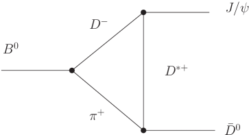
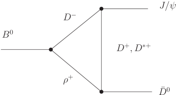
(a)	(b)
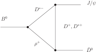
(c)	(d)
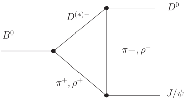
(e)

Figure 1: The hadronic loop diagrams depict the hadronic loop effect on $B^{0}\to J/\psi\bar{D}^{0}$.

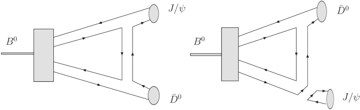
Figure 2: Left-hand and right-hand sides diagrams respectively correspond to the OZI allowed and OZI forbidden diagrams for the hadronic loop diagrams for decay of $B^{0}\to J/\psi\bar{D}^{0}$.

The effective Lagrangians at the hadron-hadron vertices in Ref. Lagarangian are

$$\mathcal{L}_{\psi DD} = ig_{\psi DD}\psi_{\mu}\left(\partial^{\mu}D\bar{D}-D\partial^{\mu}\bar{D}\right),$$ (1)

$${\mathcal{L}}_{\psi D^{*}D^{*}} = -ig_{\psi D^{*}D^{*}}\Bigl{\{}\psi^{\mu}\left(\partial_{\mu}D^{*\nu}\bar{D}_{\nu}^{*}-D^{*\nu}\partial_{\mu}\bar{D}_{\nu}^{*}\right)$$ (2)

$$+\left(\partial_{\mu}\psi_{\nu}D^{*\nu}-\psi_{\nu}\partial_{\mu}D^{*\nu}\right)\bar{D}^{*\mu}$$

$$+D^{*\mu}\left(\psi^{\nu}\partial_{\mu}\bar{D}^{*}_{\nu}-\partial_{\mu}\psi_{\nu}\bar{D}^{*\nu}\right)\Bigr{\}},$$

$${\mathcal{L}}_{\psi D^{*}D} = -g_{\psi D^{*}D}\varepsilon^{\mu\nu\alpha\beta}\partial_{\mu}\psi_{\nu}\left(\partial_{\alpha}D^{*}_{\beta}\bar{D}+D\partial_{\alpha}\bar{D}^{*}_{\beta}\right),$$ (3)

$${\mathcal{L}}_{D^{*}D\pi} = ig_{D^{*}D\pi}\left(D_{\mu}^{*}\partial^{\mu}\pi\bar{D}-D\partial^{\mu}\pi\bar{D}^{*}_{\mu}\right),$$ (4)

$${\mathcal{L}}_{D^{*}D^{*}\pi} = -g_{D^{*}D^{*}\pi}\varepsilon^{\mu\nu\alpha\beta}\partial_{\mu}D^{*}_{\nu}\pi\partial_{\alpha}\bar{D}^{*}_{\beta},$$ (5)

$${\mathcal{L}}_{DD\rho} = ig_{DD\rho}\left(D\rho^{\mu}\partial_{\mu}\bar{D}-\partial_{\mu}D\rho^{\mu}\bar{D}\right),$$ (6)

$${\mathcal{L}}_{D^{*}D\rho} = -g_{D^{*}D\rho}\varepsilon^{\mu\nu\alpha\beta}\left(D\partial_{\mu}\rho_{\nu}\partial_{\alpha}\bar{D}^{*}_{\beta}+\partial_{\mu}D^{*}_{\nu}\partial_{\alpha}\rho_{\beta}\bar{D}\right).$$

Here $\varepsilon_{0123}=+1$, $\pi=\tau\cdot{\pi}$, $\rho={\tau}\cdot{\rho}$. The definitions of the charmed meson iso-doublets are

$$\bar{D}^{T} = \left(\bar{D}^{0},D^{-}\right),\qquad D=\left(D^{0},D^{+}\right),$$

$$\bar{D}^{*T} = \left(\bar{D}^{*0},D^{*-}\right),\qquad D^{*}=\left(D^{*0},D^{*+}\right).$$ (8)

We will present the values of the necessary coupling constants in the section for the numerical computations.

With the above preparation, we can write out the decay amplitude involving contributions from the diagrams of Fig. 1 in terms of the Cutkosky Cutting Rules. For the process $B^{0}\to D^{-}(p_{1})\pi^{+}(p_{2})\to J/\psi(p_{3},\epsilon_{3})\bar{D}^{0}(p_{4})$ where as shown in Fig. 1 the vector-meson $D^{*+}$ is exchanged at t-channel, the resultant amplitude is

$${Abs}^{(a)}$$

$$=\frac{1}{2}\int\frac{d^{3}p_{1}}{(2\pi)^{3}2E_{1}}\frac{d^{3}p_{2}}{(2\pi)^{3}2E_{2}}(2\pi)^{4}\delta^{4}(p_{B}-p_{1}-p_{2})$$

$$\quad\times A(B^{0}\to D^{-}\pi^{+})(-i)g_{\psi D^{*}D}\varepsilon^{\mu\nu\alpha\beta}(-i)p_{3\mu}\epsilon_{3\nu}$$

$$\quad\times[-i(p_{3}-p_{1})_{\alpha}]i^{2}\sqrt{2}g_{D^{*}D\pi}(ip_{2}^{\xi})$$

$$\quad\times\Big{(}-g_{\xi\beta}+\frac{q_{\xi}q_{\beta}}{m_{D^{*}}^{2}}\Big{)}\frac{i}{q^{2}-m_{D^{*}}^{2}}\mathcal{F}^{2}[q^{2},m^{2}_{D^{*}}].$$ (9)

The amplitudes of the mode $B^{0}\to D^{-}(p_{1})\rho^{+}(p_{2},\epsilon_{\rho})\to J/\psi(p_{3},\epsilon_{3})\bar{D}^{0}(p_{4})$ where $D^{+}$ and $D^{*+}$ are exchanged respectively, read as

$${Abs}^{(b-1)}$$

$$=\frac{1}{2}\int\frac{d^{3}p_{1}}{(2\pi)^{3}2E_{1}}\frac{d^{3}p_{2}}{(2\pi)^{3}2E_{2}}(2\pi)^{4}\delta^{4}(p_{B}-p_{1}-p_{2})$$

$$\quad\times A(B^{0}\to D^{-}\rho^{+})i^{2}g_{\psi DD}\epsilon_{3\mu}[i(p_{3}-p_{1})^{\mu}-ip_{1}^{\mu}]$$

$$\quad\times i^{2}\sqrt{2}g_{DD\rho}[(-i)p_{4\nu}-(-i)(p_{3}-p_{1})_{\nu}]$$

$$\quad\times\Big{(}-g^{\nu\xi}+\frac{p_{2}^{\nu}p_{2}^{\xi}}{m^{2}_{\rho}}\Big{)}\frac{i}{q^{2}-m_{D}^{2}}\mathcal{F}^{2}[q^{2},m^{2}_{D}]$$ (10)

and

$${Abs}^{(b-2)}$$

$$=\frac{1}{2}\int\frac{d^{3}p_{1}}{(2\pi)^{3}2E_{1}}\frac{d^{3}p_{2}}{(2\pi)^{3}2E_{2}}(2\pi)^{4}\delta^{4}(p_{B}-p_{1}-p_{2})$$

$$\quad\times A(B^{0}\to D^{-}\rho^{+})(-i)g_{\psi D^{*}D}\varepsilon^{\mu\nu\alpha\beta}(-i)p_{3\mu}\epsilon_{3\nu}$$

$$\quad\times[-i(p_{3}-p_{1})_{\alpha}](-i)\sqrt{2}g_{D^{*}D\rho}\varepsilon^{\sigma\xi\tau\chi}$$

$$\quad\times(-i)(p_{3}-p_{1})_{\sigma}(i)p_{2\tau}\Big{(}-g_{\xi\beta}+\frac{q_{\xi}q_{\beta}}{m_{D^{*}}^{2}}\Big{)}$$

$$\quad\times\Big{(}-g_{\chi\lambda}+\frac{p_{2\chi}p_{2\lambda}}{m_{D^{*}}^{2}}\Big{)}\frac{i}{q^{2}-m_{D^{*}}^{2}}\mathcal{F}^{2}[q^{2},m^{2}_{D^{*}}].$$ (11)

For Fig. 1 (c), the amplitude of $B^{0}\to D^{*-}(p_{1},\epsilon_{D^{*+}})\pi^{+}(p_{2})\to J/\psi(p_{3},\epsilon_{3})\bar{D}^{0}(p_{4})$ where $D^{*+}$ is exchanged at t-channel, is

$${Abs}^{(c)}$$

$$=\frac{1}{2}\int\frac{d^{3}p_{1}}{(2\pi)^{3}2E_{1}}\frac{d^{3}p_{2}}{(2\pi)^{3}2E_{2}}(2\pi)^{4}\delta^{4}(p_{B}-p_{1}-p_{2})$$

$$\quad\times A(B^{0}\to D^{*-}\pi^{+})(-i^{2})g_{\psi D^{*}D^{*}}[i(p_{3}-2p_{1})\cdot\epsilon_{3}g_{\mu\nu}$$

$$\quad\times-i(2p_{3}-p_{1})_{\nu}\epsilon_{3\mu}+i(p_{1}+p_{3})_{\mu}\epsilon_{3\nu}]$$

$$\quad\times i^{2}\sqrt{2}g_{D^{*}D\pi}(ip_{2\alpha})\Big{(}-g^{\alpha\nu}+\frac{p_{1}^{\alpha}p_{1}^{\nu}}{m^{2}_{D^{*}}}\Big{)}$$

$$\quad\times\Big{(}-g^{\mu\lambda}+\frac{q^{\mu}q^{\lambda}}{m_{D^{*}}^{2}}\Big{)}\frac{i}{q^{2}-m_{D^{*}}^{2}}\mathcal{F}^{2}[q^{2},m^{2}_{D^{*}}].$$ (12)

The amplitudes of $B^{0}\to D^{*-}(p_{1},\epsilon_{D^{*+}})\rho^{+}(p_{2},\epsilon_{\rho})\to J/\psi(p_{3},\epsilon_{3})\bar{D}^{0}(p_{4})$ where $D^{+}$ and $D^{*+}$ are exchanged respectively are

$${Abs}^{(d-1)}$$

$$=\frac{1}{2}\int\frac{d^{3}p_{1}}{(2\pi)^{3}2E_{1}}\frac{d^{3}p_{2}}{(2\pi)^{3}2E_{2}}(2\pi)^{4}\delta^{4}(p_{B}-p_{1}-p_{2})$$

$$\quad\times A(B^{0}\to D^{*-}\rho^{+})(-i)g_{\psi D^{*}D}\varepsilon^{\lambda\tau\sigma\gamma}(-i)p_{3\lambda}\epsilon_{3\tau}$$

$$\quad\times(i)p_{1\sigma}(i^{2})\sqrt{2}g_{DD\rho}[(-i)p_{4\xi}-(-i)(p_{3}-p_{1})_{\xi}]$$

$$\quad\times\Big{(}-g^{\mu\xi}+\frac{p_{2}^{\mu}p_{2}^{\xi}}{m^{2}_{\rho}}\Big{)}\Big{(}-g_{\gamma}^{\nu}+\frac{p_{1\gamma}p_{1}^{\nu}}{m_{D^{*}}^{2}}\Big{)}$$

$$\quad\times\frac{i}{q^{2}-m_{D}^{2}}\mathcal{F}^{2}[q^{2},m^{2}_{D}]$$ (13)

and

$${Abs}^{(d-2)}$$

$$=\frac{1}{2}\int\frac{d^{3}p_{1}}{(2\pi)^{3}2E_{1}}\frac{d^{3}p_{2}}{(2\pi)^{3}2E_{2}}(2\pi)^{4}\delta^{4}(p_{B}-p_{1}-p_{2})$$

$$\quad\times A(B^{0}\to D^{*-}\rho^{+})(-i^{2})g_{\psi D^{*}D^{*}}[i(p_{3}-2p_{1})\cdot\epsilon_{3}g_{\lambda\tau}$$

$$\quad\times-i(2p_{3}-p_{1})_{\tau}\epsilon_{3\lambda}+i(p_{1}+p_{3})_{\lambda}\epsilon_{3\tau}]$$

$$\quad\times(-i)\sqrt{2}g_{D^{*}D\rho}\varepsilon^{\sigma\xi\omega\chi}(-i)(p_{3}-p_{1})_{\sigma}(i)p_{2\omega}$$

$$\quad\times\Big{(}g^{\nu\tau}+\frac{p_{1}^{\nu}p_{1}^{\tau}}{m_{D^{*}}^{2}}\Big{)}\Big{(}-g^{\mu}_{\chi}+\frac{p_{2}^{\mu}p_{2\chi}}{m_{\rho}^{2}}\Big{)}$$

$$\quad\times\Big{(}-g_{\xi}^{\lambda}+\frac{q_{\xi}q^{\lambda}}{m^{2}_{D^{*}}}\Big{)}\frac{i}{q^{2}-m_{D^{*}}^{2}}\mathcal{F}^{2}[q^{2},m^{2}_{D^{*}}].$$ (14)

In the above expressions, $\mathcal{F}[q^{2},m_{i}^{2}]$ denotes the form factor (FF), which reflects the structure effect at the effective interaction vertices. In this work, following Ref. HY-Chen we take the monopole form for FF as

$$\mathcal{F}[q^{2},m_{i}^{2}]=\Big{(}\frac{\Lambda^{2}-m_{i}^{2}}{\Lambda^{2}-q^{2}}\Big{)},$$ (15)

where the phenomenological parameter $\Lambda$ can be parameterized as

$$\Lambda=m_{i}^{2}+\alpha\Lambda_{QCD}.$$ (16)

$m_{i}$ stands as the mass of the exchanged meson at t-channel which is depicted in Fig. 1.

The decay amplitude of $B^{0}\to J/\psi\bar{D}^{0}$ via the hadronic loop diagrams is

$$\mathcal{M}[B^{0}\to D^{(*)-}\pi^{+}(\rho^{+})\to J/\psi\bar{D}^{0}]$$

$$=Abs^{(a)}+Abs^{(b-1)}+Abs^{(b-2)}$$

$$\quad+Abs^{(c)}+Abs^{(d-1)}+Abs^{(d-2)}.$$ (17)

III $B\to D^{(*)}\pi(\rho)$ decays in the factorization approach

In this section, let us turn to study $B\to D^{(*)}\pi(\rho)$. We can reliably apply the factorization which has been proved to be valid to all orders of the strong coupling constant in the heavy quark limit BBNS ; SCET , to calculate the amplitude. The essential non-perturbative quantities are light meson ($\pi,\rho$) decay constants and $B\to D(D^{*})$ transition form factors.

The decay constants for pseudoscalar ($P$) and vector ($V$) mesons are defined as

$$\langle P(q)|A_{\mu}|0\rangle = -if_{P}q_{\mu},$$

$$\langle V(q,\epsilon)|V_{\mu}|0\rangle = f_{V}m_{V}\epsilon^{*}_{\mu}.$$ (18)

where vector and axial vector currents are $V_{\mu}=\bar{q}_{1}\gamma_{\mu}q_{2}$ and $A_{\mu}=\bar{q}_{1}\gamma_{\mu}\gamma_{5}q_{2}$ respectively and $\epsilon$ is the polarization vector of $V$.

The $B\rightarrow H\left(H=D,\ D^{*}\right)$ transition form factors are conventionally parameterized as in CGW

$$\langle D|V_{\mu}|\bar{B}\rangle=F_{1}(q^{2})\Big{\{}P_{\mu}-\frac{P\cdot q}{q^{2}}q_{\mu}\Big{\}}$$

$$\qquad\quad\qquad+\frac{P\cdot q}{q^{2}}F_{0}(q^{2})\,q_{\mu},$$ (19)

$$\langle D^{*}(\epsilon)|V_{\mu}|\bar{B}\rangle=\frac{V(q^{2})}{m_{B}+m_{D^{*}}}\varepsilon_{\mu\alpha\beta\rho}\epsilon^{*\alpha}P^{\beta}q^{\rho},$$ (20)

$$\langle D^{*}(\epsilon)|A_{\mu}|\bar{B}\rangle=i\Big{[}2m_{D^{*}}A_{0}(q^{2})\frac{\epsilon^{*}\cdot q}{q^{2}}q_{\mu}$$

$$\qquad\quad+(m_{B}+m_{D^{*}})A_{1}(q^{2})\Big{(}\epsilon_{\mu}^{*}-\frac{\epsilon^{*}\cdot q}{q^{2}}q_{\mu}\Big{)}.$$

$$\qquad\quad-A_{2}(q^{2})\frac{\epsilon^{*}\cdot q}{m_{B}+m_{D^{*}}}\Big{(}P_{\mu}-\frac{P\cdot q}{q^{2}}q_{\mu}\Big{)}\Big{]},$$ (21)

where $P=p_{B}+p_{D^{(*)}}$, $q=p_{B}-p_{D^{(*)}}$ and $P\cdot q=m^{2}_{B}-m^{2}_{D^{(*)}}$.

The decay amplitudes for $B\to D^{(*)}\pi(\rho)$ are given as

$$A(B^{0}\to D^{-}\pi^{+})$$

$$=\frac{G_{F}}{\sqrt{2}}V_{cb}^{*}V_{ud}a_{1}\left\{if_{\pi}(m^{2}_{B}-m^{2}_{D})F^{BD}_{0}(m^{2}_{\pi})\right\},$$ (22)

$$A(B^{0}\to D^{-}\rho^{+})$$

$$=\frac{G_{F}}{\sqrt{2}}V_{cb}^{*}V_{ud}a_{1}\left\{2f_{\rho}\,m_{\rho}F_{1}^{BD}(m_{\rho}^{2})(\varepsilon_{\rho}^{*}\cdot p_{{}_{B}})\right\},$$ (23)

$$A(B^{0}\to D^{*-}\pi^{+})$$

$$=\frac{G_{F}}{\sqrt{2}}V_{cb}^{*}V_{ud}a_{1}\left\{2f_{\pi}\,m_{D^{*}}A_{0}^{BD^{*}}(m_{\pi}^{2})(\varepsilon_{D^{*}}^{*}\cdot p_{{}_{B}})\right\},$$

$$A(B^{0}\to D^{*-}\rho^{+})$$

$$=\frac{G_{F}}{\sqrt{2}}V_{cb}^{*}V_{ud}a_{1}\Bigg{\{}-if_{{\rho}}m_{{\rho}}\Bigg{[}(\varepsilon^{*}_{D^{*}}\cdot\varepsilon^{*}_{\rho})(m_{B}$$

$$\quad+m_{D^{*}})A_{1}^{BD^{*}}(m_{\rho}^{2})$$

$$\quad-(\epsilon^{*}_{D^{*}}\cdot p_{\rho})(\epsilon^{*}_{\rho}\cdot p_{{}_{D^{*}}}){2A_{2}^{BD^{*}}(m_{\rho}^{2})\over(m_{B}+m_{D^{*}})}$$

$$\quad+i\epsilon_{\mu\nu\alpha\beta}\varepsilon^{*\mu}_{\rho}\varepsilon^{*\nu}_{D^{*}}p^{\alpha}_{\rho}p^{\beta}_{D^{*}}\,{2V^{B{D^{*}}}(m_{\rho}^{2})\over(m_{B}+m_{D^{*}})}\Bigg{]}\Bigg{\}}.$$ (25)

IV Numerical result

The relevant input parameters which are employed in this work include: $m_{B^{0}}=5279.4$ MeV, $m_{D^{0}}=1864.5$ MeV, $m_{J/\psi}=3096.9$ MeV, $m_{D^{\pm}}=1869.3$ MeV, $m_{D^{*\pm}}=2010.0$ MeV, $m_{\pi^{\pm}}=139.6$ MeV, $m_{\rho^{\pm}}=775.5$ MeV, $G_{F}=1.16637\times 10^{-5}$ GeV^-1, $V_{ud}=0.974$, $V_{cb}=41.6\times 10^{-3}$ PDG ; $g_{D^{*}D\pi}=8.84$, $g_{D^{*}D^{*}\pi}=9.08$ GeV^-1, $g_{\psi DD}=g_{\psi D^{*}D^{*}}=7.71$, $g_{\psi D^{*}D}=8.64$, $g_{D^{*}D^{*}\rho}=g_{DD\rho}=2.52$, $g_{D^{*}D\rho}=2.82$ GeV^-1 Lagarangian ; $f_{\pi}=132$ MeV and $f_{\rho}=216$ MeV CCH .

The Wilson coefficient $a_{1}$ has been calculated up to the next-to-leading order BBNS and we take the value

$$a_{1}=1.05.$$ (26)

The momentum dependence of the transition form factors in eqs. (22)-(25) possess the pole structures CCH as

$$F(q^{2})=\frac{F(0)}{1-a\zeta+b\zeta^{2}}$$ (27)

with $\zeta=q^{2}/m_{B}^{2}$. $F(0)$, $a$ and $b$ are obtained by fitting data and their values are shown in Table 1.

$F$	$F(0)$	$a$	$b$
$F_{0}^{BD}$	0.67	0.65	0.00
$F_{1}^{BD}$	0.67	1.25	0.39
$A_{0}^{BD^{*}}$	0.64	1.30	0.31
$A_{1}^{BD^{*}}$	0.63	0.65	0.02
$A_{2}^{BD^{*}}$	0.61	1.14	0.52
$V^{BD^{*}}$	0.75	1.29	0.45

Table 1: The values of $F(0)$, $a$ and $b$ in the form factors of $B\to D^{(*)}$ CCH .

With the values given in Table 1, one obtains $F_{0}^{BD}(m^{2}_{\pi})=0.67$, $F_{1}^{BD}(m^{2}_{\rho})=0.69$, $A_{0}^{BD^{*}}(m^{2}_{\pi})=0.64$, $A_{1}^{BD^{*}}(m^{2}_{\rho})=0.64$, $A_{2}^{BD^{*}}(m^{2}_{\rho})=0.63$, $V^{BD^{*}}(m^{2}_{\rho})=0.77$, which will be applied to the later numerical calculation.

In Fig. 3, we show the dependence of the branching ratio of $B^{0}\to J/\psi\bar{D}^{0}$ on the phenomenological parameter $\alpha$ in eq. 16, which spans a range $\alpha=1\sim 3$. Furthermore, Table 2 presents the branching ratio of $B^{0}\to J/\psi\bar{D}^{0}$ with some typical values of $\alpha$.

Figure 3: The variation of the branching ratio of $B^{0}\to J/\psi\bar{D}^{0}$ with $\alpha=1\sim 3$.

$\alpha$	1.0	1.5	2.0	2.5	3.0
$B[B^{0}\to J/\psi\bar{D}^{0}]$
$(\times 10^{-5})$	$0.13$	$0.54$	$1.4$	$3.0$	$5.2$

Table 2: The branching ratio of $B^{0}\to J/\psi\bar{D}^{0}$ corresponding to several typical values of $\alpha$.

V Conclusion and discussion

In this work, we calculate the contribution of the FSI, i.e. inelastic rescattering processes to the branching ratio of $B^{0}\to J/\psi\bar{D}^{0}$ and find that it spans a relatively wider range of $10^{-6}\sim 10^{-5}$ which is obviously larger than the theoretically predicted value $10^{-8}$ EMY and comparable with the pQCD prediction of $10^{-6}$ LLQ , moreover, it is also noted that as $\alpha=3$ is taken, it can be close to the experimental upper bounds. We hope that the Babar and Belle collaborations will further investigate the process and carry out more accurate measurements. Then not only an upper bounds will be given, but also a rather precise branching ratio can be obtained.

The significance of this investigation to the present theoretical frameworks is obvious as discussed in the section of introduction. Since in the process the linear momentum of the final products is not large, there can exist a region where the exchanged gluon is soft and application of pQCD might fail. This region should be fully governed by the non-perturbative QCD effects which are not involved in the conventional pQCD calculations, even though phenomenological wavefunctions of the hadrons can partly cover such effects. Thus we consider the FSI effects as an additional contribution to that of pQCD evaluation. However, on another aspect, one cannot indeed determine the range where pQCD fails and this is exactly the goal of this work.

As noticed, there exist some phenomenological parameters in our calculations on FSI effects, such as $\alpha$ or $\Lambda$ in eq. (16) and other uncertainties which are coming from the employed data, therefore, we can only trust the results to the order of magnitude. However, the largeness of the contribution of the FSI should draw our attention because it may change the whole scenario. In fact, an accurate measurement can provide an ideal field for testing validity of pQCD. Since the FSI can result in a branching ratio as large as $10^{-6}\sim 10^{-5}$, there is a region where the pQCD prediction and the contribution of the FSI have the same order, thus it is hard to clearly identify individual contribution from both mechanism, unless accurate measured data are available. On other aspect, under the assumption that the present pQCD calculation is trustworthy to a certain accuracy, it is not hopeless to determine their fractions because the two factories indeed have ability to carry out such precise, but difficult measurements.

More concretely, if the future measurement confirmed a smaller branching ratio of about $10^{-6}$, then one would make a careful analysis to distinguish between the two kinds of contributions. Furthermore, if the data are basically consistent with the pQCD predicted value, it is indicated that pQCD works well, even though there might be a range where application of pQCD is dubious. In other words, for that case, the range where pQCD fails, does not make dominant contribution and the whole theoretical framework should cover a much wider application range than was expected. Then we have to re-adjust the input parameters for calculating the FSI or set a more stringent constraint on them. It would be very helpful for gaining knowledge on the FSI which plays important roles in many decay and production processes.

By contraries, if the future measurements on $B^{0}\to J/\psi\bar{D}^{0}$ confirm that the branching ratio is obviously larger than $10^{-6}$, the fact would indicate that the region where pQCD fails, is important and should be re-considered. In that case, we can conclude that one must be careful as he applies the pQCD to evaluate physical processes with low energy scales. And the FSI may be a possible solution to the discrepancy. If it is true, a byproduct would be that one can further investigate details about the methods for calculation on the FSI effects and determine the concerned parameters, since the ”contamination” from the direct process which is evaluated in terms of pQCD is relatively small.

As a conclusion, we would urge our experimental colleagues to make a more accurate measurement on this process because its significance to our theory is obvious.

References

• (1) CLEO Collaboration, R.Balest et al., Phys. Rev. D 52, 2661(1995).
• (2) Belle Collaboration, S.E. Schrenk, in ICHEP 2000: Proceeding,, edited by C.S. Lim and T. Yamanaka (World Scientific, Singapore,2001).
• (3) BABAR Collaboration, B. Aubert, et al., Phys.Rev. D 67, 032002(2003).
• (4) S.J. Brodsky and F.S. Navarra, Phys. Lett. B 411, 152 (1997).
• (5) C.H. Chang and W.S. Hou, Phys. Rev. D 64, 071501 (2001); C.K. Chua, W.S. Hou and G.G. Wong, Phys. Rev. D 68, 054012 (2003).
• (6) G. Eilam, M. Ladisa and Y.D. Yang, Phys. Rev. D 65, 037504 (2002).
• (7) BABAR Collaboration, B. Aubert et al., Phys. Rev. D 71, 091103 (2005).
• (8) Belle Collaboration, L. M. Zhang, et al., Phys. Rev. D 71, 091107 (2005).
• (9) Y. Li, C.D. Lu and C.F. Qiao, Phys. Rev. D 73, 094006 (2006).
• (10) X. Liu, X.Q. Zeng and X.Q. Li, Phys. Rev. D 74, 074003 (2006).
• (11) N. Isgur, K. Maltman, J. Weinstein and T. Barnes, Phys. Rev. Lett. 64, 161 (1990); M.P. Locher, V.E. Markusin and H.Q. Zheng, Report No. PSI-PR-96-13 (unpublished); H. Lipkin, Nucl. Phys. B 244, 147 (1984); H. Lipkin, Phys. Lett. B 179, 278 (1986); H. Lipkin, Nucl. Phys. B 291, 720 (1987); H.J. Lipkin and B.S. Zou, Phys. Rev. D 53, 6693 (1996); P. Geiger and N. Isgur, Phys. Rev. Lett. 67, 1066 (1991); V.V. Anisovich, D.V. Bugg, A.V. Sarantsev and B.S. Zou, Phys. Rev. D 51, R4619 (1995); D.S. Du, X.Q. Li, Z.T. Wei and B.S. Zou, Eur. Phys. J. A 4, 91 (1999); Y.S. Dai, D.S. Du, X.Q. Li, Z.T. Wei and B.S. Zou, Phys. Rev. D 60, 014014 (1999); S.L. Chen, X.H. Guo, X.Q. Li and G.L.Wang, Commun. Theor. Phys. 40, 563 (2003); C.D. Lu, Y.L. Shen and W. Wang, Phys. Rev. D 73, 034005 (2006).
• (12) X. Liu and X.Q. Li, arXiv: 0707.0919 [hep-ph], Phys. Rev. D (in press); X. Liu, B. Zhang and S.L. Zhu, Phys. Lett. B 645 185-188 (2007); X. Liu, B. Zhang, L.L. Shen, S.L. Zhu, Phys. Rev. D 75, 074017 (2007).
• (13) H.Y. Cheng, C.K. Chua and A. Soni, Phys. Rev. D71, 014030 (2005).
• (14) Y. Oh, T. Song and S.H. Lee, Phys. Rev. C 63, 034901.
• (15) M. Beneke, G. Buchalla, M. Neubert and C.T. Sachrajda, Nucl. Phys. B 591, 313 (2000).
• (16) C.W. Bauer, D. Pirjol and I.W. Stewart, Phys. Rev. Lett 87, 201806 (2001).
• (17) C.H. Chen, C.Q. Geng and Z.T. Wei, Eur. Phys. J. C 46, 367 (2006).
• (18) W.M. Yao et al., Particle Data Group, J. Phys. G 33, 1 (2006).
• (19) H.Y. Cheng, C.K. Chua, C.W. Hwang, Phys. Rev. D 69, 074025 (2004).