Physics-based mathematical models for quantum devices via experimental system identification

Abstract

We consider the task of intrinsic control system identification for quantum devices. The problem of experimental determination of subspace confinement is considered, and simple general strategies for full Hamiltonian identification and decoherence characterization of a controlled two-level system are presented.

1 Introduction

Advances in nano-fabrication are increasingly enabling us to create nano-scale devices that exhibit non-classical or quantum-mechanical behaviour. Such quantum devices are of great interest as they may pave the way for a new generation of quantum technology with various applications from quantum metrology to quantum information processing. However, to create quantum devices that perform useful functions, we must be able to understand their behaviour, and have effective means to controllably manipulate it. Analysis of system dynamics and the design of effective control strategies is almost impossible without the availability of sufficiently accurate mathematical models of the device. While these models should capture the essential features of the device, to be useful, they must also be computationally tractable, and preferably as simple as possible.

There are different approaches to deal with this problem. One, which we shall refer to as a first-principles approach, involves constructing model Hamiltonians based on reasonable assumptions about the relevant physical processes governing the behaviour of the system, making various simplifications, and solving the Schrodinger equation in some form, usually using numerical techniques such as finite element or functional expansion methods. The empirical approach, on the other hand, starts with experimental data and observations to construct a model of the system. In practice both approaches are needed to deal with complex systems. First-principle models are crucial to elucidate the fundamental physics that governs a system or device, but experimental data is crucial to account for the many unknowns that result in variability of the characteristics of the system, which is often difficult to predict or explain theoretically. For instance, ‘manufactured’ systems such as artificial quantum dot ‘atoms’ and ‘molecules’ vary considerably in size, geometry, internal structure, etc, and sometimes even small variations can significantly alter their behaviour.

In this paper we will focus on constructing mathematical models solely from experimental data without any prior knowledge of the specifics of the system, an approach one might call black-box system identification. We will restrict ourselves to quantum systems whose essential features can be captured by low-dimensional Hilbert space models. For instance, a quantum dot molecule such as the Silicon double quantum dot system in Fig. 1 may consist of millions of individual atoms with many degrees of freedom, but the observable dynamics may be well described by overall charge distribution states in the quantum dot molecule. Taking these charge distribution states as basis states for a Hilbert space $\mathcal{H}$, the observable dynamics of the system is governed by a Hamiltonian operator acting on $\mathcal{H}$, and possibly additional non-Hermitian operators to account for dissipative effects if the system is not completely isolated from its environment. If the dimension of the Hilbert space $\mathcal{H}$ is huge then complete characterization of the Hamiltonian and dissipation operators may be a hopeless task, but in certain cases the dynamics of interest takes place in low-dimensional Hilbert space $\mathcal{H}$, or we may in fact wish to design a device whose dynamics can be described by a low-dimensional Hilbert space model, as is the case in quantum information processing 00Nielsen , where we desire to create systems that act as quantum bits, for example.

The paper is organized as follows. We start with a general description of the basic assumptions we make about the system to be modelled and the type of measurements and experiments upon which our characterization protocols are based. In section 3 we discuss the problem of subspace confinement, i.e., how to experimentally characterize how well the dynamics of system is confined to a low-dimensional subspace such as a two-dimensional (qubit) Hilbert space. In section 4 we present general protocols for identifying Hamiltonian and decoherence parameters for controlled qubit-like systems. We conclude with a discussion of generalizations and open problems.

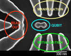
Figure 1: Simple charge ‘qubit’ device: Trench-isolated Silicon double quantum dot molecule fabricated using e-beam lithography, controlled by several DC-gate electrodes, with a single electron transistor for charge readout (Hitachi Cambridge Labs) PhysRevLett.95.090502 .

2 General Modelling Assumptions

We start with a generic model assuming only that the state of the system can be represented by a density operator (i.e., a positive operator of trace one) $\hat{\rho}$ acting on a Hilbert space $\mathcal{H}$ of dimension $N$, and that its evolution is governed by the quantum Liouville equation (in units such that $\hbar=1$):

$$\frac{d}{dt}\hat{\rho}(t)=-\rmi[\hat{H},\hat{\rho}(t)]+\mathcal{L}_{D}[\hat{\rho}(t)],$$ (1)

where $\hat{H}$ is an effective Hamiltonian and $\mathcal{L}_{D}$ a super-operator that accounts for dissipative effects due to environmental influences, etc. Initially, all that is known about $\hat{H}$ and $\mathcal{L}_{D}$ is that $\hat{H}$ is a Hermitian operator on $\mathcal{H}$, and $\mathcal{L}_{D}$ a completely positive super-operator acting on density matrices $\hat{\rho}(t)$, although we may make some additional assumptions about the structure of $\hat{H}$ or $\mathcal{L}_{D}$. For instance, we shall generally assumes $\mathcal{L}_{D}$ to be of Kossakowski-Sudarshan-Lindblad form 76Lindblad ; 76Gorini :

$$\mathcal{L}_{D}[\hat{\rho}(t)]=\sum_{k=1}^{N^{2}-1}\gamma_{k}\mathcal{D}[\hat{V}_{k}]\hat{\rho}(t)$$ (2)

where the super-operators $\mathcal{D}[\hat{V}_{k}]$ are defined by

$$\mathcal{D}[A]B=ABA^{\dagger}-(A^{\dagger}AB+BA^{\dagger}A)/2,$$ (3)

$\hat{V}_{k}$ are (generally non-Hermitian) operators on $\mathcal{H}$ and $\gamma_{k}$ are positive real numbers.

If the system is subject to dynamic control, then the Hamiltonian (and sometimes the relaxation operators $\hat{V}_{k}$) are not fixed but dependent on external control fields, which we shall denote by ${\bf f}(t)$. In the simplest case, we may assume a linear dependence of the Hamiltonian on the controls

$$\hat{H}[{\bf f}(t)]=\hat{H}_{0}+\sum_{m=1}^{M}f_{m}(t)\hat{H}_{m},$$ (4)

where the $\hat{H}_{m}$ are fixed Hermitian operators on $\mathcal{H}$ and the reservoir operators $\hat{V}_{k}$ are constant.

The ultimate objective of characterization is to identify the operators $\hat{H}[{\bf f}(t)]$ (or $\hat{H}_{m}$) and $\mathcal{L}_{D}$ by performing suitable experiments on the system. This task would be simplified if we could assume that the system can be prepared in an arbitrary initial state $\hat{\rho}_{0}$, and that we can perform generalized measurements or projective measurements in arbitrary bases at any time—but these requirements are generally unrealistic. For example, our ability to perform measurements on the system prior to characterization is limited by the direct readout processes available, and often we only have a single, basic sensor such as a single electron transistor (SET) NAT406p1039 providing relatively limited information about the charge distribution in a quantum dot molecule, or detection may be accomplished via a readout transition that involves coupling one state of the system to a fluorescent read-out state, e.g., via a laser, etc. Furthermore, preparation of non-trivial states generally depends on knowledge of the operators $\hat{H}[{\bf f}(t)]$ and $\mathcal{L}_{D}$, the very information about the system we are trying to obtain. These practical restrictions rule out conventional quantum state or process tomography techniques, which presume the ability to measure the system in different measurement bases and prepare it in different initial states to obtain sufficient information to reconstruct the quantum state or process JMO44p2455 ; PRL78p0390 ; JMP44p0528 ; PhysRevA.66.012303 ; qph0411093 .

In this paper we consider a rather typical experimental scenario, where we are limited to measurements of a fixed observable and evolution under a Hamiltonian that can be modified by varying certain control settings. For the most part, we restrict ourselves further to piecewise constant controls. The only assumption on the measurement process we make is that it can be formally represented by some Hermitian operator $\hat{A}$ with $N$ eigenvalues corresponding to measurement outcomes $\lambda_{n}$, i.e., that it has a spectral decomposition of the form

$$\hat{A}=\sum_{n=1}^{N}\lambda_{n}|n\rangle\langle n|.$$ (5)

This measurement also serves as initialization of the system as outcome $\lambda_{n}$ means that the system will be left in an eigenstate $|n\rangle$ associated with the eigenvalue $\lambda_{n}$. If $\hat{A}$ has $N$ unique eigenvalues, i.e., all eigenvalues occur with multiplicity one, then the measurement is sufficient to initialize the system in a unique state; if it has degenerate eigenvalues associated with eigenspaces of dimension greater $>1$ then some measurement outcomes will not determine the state uniquely.

Following the idea of intrinsic characterization, our objective is to extract information about the system without recourse to any external resources, i.e., using no information from measurements other than the information provided by the sensors built into the device, and no external control fields except the ability to change the settings of the built-in actuators (such as variable gate voltages) subject to constraints. Although this requirement of characterization relying only on the built-in sensors and actuators may seem excessively restrictive, excluding many forms of spectroscopy, for example, it has the advantage of simplicity (no external resources required). Moreover, external sensors and actuators may disturb the system, and thus characterization of the system in their presence may not yield an accurate picture of the dynamics in the absence of the additional apparatus.

We restrict ourselves here to systems sufficiently weakly coupled to a sufficiently large reservoir, whose dynamics can be described by adding a dissipation super-operator of the form (2) to the Hamiltonian dynamics of the subsystem of interest. Although many systems can be modelled this way, it should be noted that this approach has limitations. For example, the dynamics of a subsystem $\mathcal{H}_{S}$ that is strongly is coupled to a finite reservoir $\mathcal{H}_{R}$, such as single spin coupled to several nearby spins, can be very complicated and non-Markovian. Although non-Markovian dynamics can in principle be dealt with by allowing time-dependent relaxation operators $\hat{V}_{k}$, in such cases it is not always possible to describe the dynamics of the subsystem of interest in terms of the Hamiltonian dynamics on the subspace and a set of simple relaxation or decoherence operators. Rather, it may become necessary to consider the system $\mathcal{H}_{S}+\mathcal{H}_{R}$ and characterize its dynamics, described by a Schrodinger equation with a Hamiltonian $\hat{H}_{S+R}$, instead to obtain an accurate picture of the subsystem dynamics. The basic ideas of intrinsic characterization can be applied to this larger system, and the protocols we will describe can in principle be extended to such higher-dimensional systems, although full characterization of the system plus reservoir Hamiltonian $\hat{H}_{S+R}$ using only the built-in sensors and actuators may not be possible. The degree of characterization possible will depend on the size of the Hilbert space and the capabilities of the built-in sensors and actuators, e.g., to discriminate and manipulate different states of the larger system. Before attempting to identify the system Hamiltonian (and decoherence operators), an important first task is therefore estimating the dimension of the Hilbert space in which the dynamics takes place.

3 Characterization of subspace confinement

A fundamental prerequisite for constructing a Hilbert space model is knowledge of the underlying Hilbert space. This is a nontrivial problem as most systems have many degrees of freedom, and thus a potentially huge Hilbert space, but effective characterization of the system often depends on finding a low dimensional Hilbert space model that captures the essential features of the system. Furthermore, in applications such as quantum information processing the elementary building blocks are required to have a certain Hilbert space dimension. For example, for a quantum-dot molecule to qualify as a qubit, we must be able to isolate a two-dimensional subspace of the total Hilbert space, and be able to coherently manipulate states within this 2D subspace without coupling to states outside the subspace (leakage). This requires several characterization steps:

1. Isolation of a 2D subspace and characterization of subspace confinement;

2. Characterization of the Hamiltonian dynamics including effect of the actuators; and

3. Characterization of (non-controllable) environmental effects (dissipation).

The choice of a suitable subspace depends also on the measurement device as the measurement must be able to distinguish the basis states. Thus for a potential charge qubit device, for example, only a subspace spanned by charge states that can be reliably distinguished by the SET is a suitable candidate, and ideally there should be two (or in general $N$) orthogonal states that can be perfectly distinguished by the measurement, so that we have a well-defined reference frame (basis) $\{|0\rangle,|1\rangle,\ldots,|N\rangle\}$, and the measurement can be represented by an observable of the form (5) with $N$ distinct eigenvalues $\lambda_{n}$. Furthermore, we would like the readout process to act as a projective measurement, so that each measurement projects the state of the system onto one of the measurement basis states $|n\rangle$. The ability to perform projective measurements is not a trivial requirement, especially for solid state systems, and is not an absolute necessity as characterization protocols can be adapted to weak measurements, but projective measurements can in principle be achieved with various sensors such as rf-SETs, and we shall assume here that we are working in this regime.

After a possible subspace has been identified, it is crucial to check that the subspace is sufficiently isolated, i.e., that we can reliably initialize the system in a state in this subspace and that it remains in this subspace under both free and controlled evolution. This characterization of subspace confinement is very important. If the device is a candidate for a qubit, for example, it is essential that subspace leakage be much less than the rate of bit or phase flip errors due to imperfect control or decoherence as leakage or loss error correction protocols are considerably more demanding in terms of complexity and resources required.

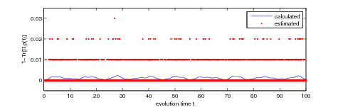
Figure 2: Leakage characterization assuming three-outcome measurement for system initialized in state $|0\rangle$. The continuous curve is the calculated value of $p_{\rm leak}(t)=1-\Tr[\Pi\hat{\rho}(t)]$, where $\Pi=|0\rangle\langle 0|+|1\rangle\langle 1|$ is the projector onto the target subspace, for a 10-level test Hamiltonian. The red dots are the estimates of $p_{\rm leak}(t)$ at the discrete times $t_{k}=(k-1)\Delta t$ with $\Delta t=0.01$, obtained by averaging over $N_{e}^{\prime}=100$ simulated experiments for each $t_{k}$. As the figure shows, the effect of the projection noise makes it difficult to obtain accurate estimates of $p_{\rm leak}(t)$ for any given $t=t_{k}$ unless $N_{e}^{\prime}$ is extremely large. However, the average leakage rate over the time interval $[0,100]$, $\bar{p}_{\rm leak}=0.11$% for both the calculated and measured values.

Characterization of subspace confinement depends on the characteristics of the sensors, i.e., the type of measurements we can perform. For our charge qubit with SET readout example, if the SET can be calibrated to be sufficiently sensitive to enable detection of states outside the chosen subspace in addition to being able to discriminate the subspace basis states $|n\rangle$, i.e., if the true measurement has (at least) $N+1$ mutually exclusive outcomes $\lambda_{n}$, $n=1,\ldots,N$ and $\lambda_{N+1}$ if the system state is outside the subspace, then the characterization of subspace confinement is relatively easy. If we perform $N_{e}$ experiments of the form

1. Initialize: Measure and record outcome $\lambda_{a}$

2. Evolve: Let the system evolve for time $t$ under some fixed Hamiltonian $H_{{\bf f}}$

3. Measure: Repeat measurement and record outcome $\lambda_{b}$

and denote by $N_{a,b}$ the number of times the measurement results for the initial and final measurements were $\lambda_{a}$ and $\lambda_{b}$, respectively, then, for $N_{e}$ sufficiently large, the leakage out of the subspace is approximately equal to the fraction of experiments for which the first measurement was $\lambda_{n}$ with $n\leq N$ and the second measurement was $N+1$, i.e.,

$$p_{\rm leak}\approx\frac{\sum_{n=1}^{N}N_{n,N+1}}{N_{e}-\sum_{n=1}^{N+1}N_{N+1,n}}.$$ (6)

Repeating the experiments for different evolution times $t$ and averaging then gives an indication of the rate of subspace leakage, e.g., if we estimate $p_{\rm leak}(t_{k})$ for $t_{k}=k\Delta t$, $k=0,\ldots,K$, then

$$\bar{p}_{\rm leak}=\frac{1}{t_{\rm max}}\int_{0}^{t_{max}}p_{\rm leak}(t)\,dt\approx\frac{1}{K+1}\sum_{k=0}^{K}p_{\rm leak}(t_{k}).$$ (7)

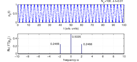
Figure 3: $p_{0}(t)$ obtained by averaging over $N_{e}=100$ simulated experiments with a 10-level test Hamiltonian and corresponding Fourier spectrum. From the 0th and 1st order peak heights we obtain $h_{0}+2h_{1}=0.9970$, which yields upper and lower bounds for $\epsilon$ of $\approx 0.0015$, although these bounds are statistically uncertain due to projection noise and discretization errors. Nonetheless, it can be verified that the actual subspace confinement for the chosen test Hamiltonian is $99.94$%, and thus the upper bound provides a reasonable estimate for the leakage.

If the SET (or other measurement process) is not sufficiently sensitive to reliably distinguish at least $N$ subspace basis states $|n\rangle$ as well as states outside the subspace, then subspace characterization is more challenging. For instance, suppose we have a 2D subspace and a sensor that can reliably detect only one state, say $|0\rangle$, a common scenario for many systems where readout transitions are used that detect only a single state. In this case the measurement outcomes are $\lambda_{0}$ or $\neg\lambda_{0}$. If the measurement is projective and the dynamics confined to a 2D subspace, we can identify $\neg\lambda_{0}$ with outcome $\lambda_{1}$ but this identification will lead to errors if the dynamics is not really confined to a 2D subspace. However, even in this case we can still estimate the level of confinement to a 2D subspace under the evolution of a Hamiltonian $\hat{H}_{{\bf f}}$ from observable coherent oscillations. For example, let

$$p_{0}(t)=|\langle 0|e^{-i\hat{H}_{{\bf f}}t}|0\rangle|^{2}$$ (8)

be the probability of obtaining outcome $\lambda_{0}$ when measuring the time-evolved state $|\Psi(t)\rangle=\exp(-it\hat{H}_{{\bf f}})|0\rangle$. If the system is initialized in the state $|0\rangle$ and the dynamics of the system under $\hat{H}_{{\bf f}}$ is perfectly confined to a two-level subspace then conservation of probability implies that the heights $h_{0}$ and $h_{1}$ of the 0th and 1st order terms in the Fourier spectrum of $p_{0}(t)$ must satisfy $h_{0}+2h_{1}=1$. We can use the deviation from this equality to bound the subspace leakage $\epsilon$ NJP7p384:

$$1-\sqrt{h_{0}+2h_{1}}\leq\epsilon\leq\frac{1}{2}(1-\sqrt{2(h_{0}+2h_{1})-1}).$$ (9)

As the upper and lower bounds depend only on the 0th and 1st order Fourier peaks, they can usually be easily determined from experimental data although finite resolution due to discretization and projection noise will reduce the accuracy of the estimates NJP7p384. Moreover, in this case $1-\epsilon$ only indicates the confinement of the system to some two-level subspace, and we must be careful as for different controls ${\bf f}$ the dynamics under $\hat{H}_{{\bf f}}$ may be confined to different two-level subspaces, in which case the system cannot be considered a proper qubit. For instance, for the 10-level test Hamiltonian

$$\hat{H}_{\rm test}=\begin{pmatrix}1.3701&1.0000&0.0093&0.0055&0.0112&0.0068&0.0119&0.0084&0.0065&0.0087\\ 1.0000&1.5561&0.0109&0.0132&0.0067&0.0061&0.0081&0.0051&0.0105&0.0029\\ 0.0093&0.0109&1.6603&0.0034&0.0161&0.0100&0.0101&0.0123&0.0115&0.0055\\ 0.0055&0.0132&0.0034&1.9112&0.0136&0.0072&0.0093&0.0062&0.0133&0.0101\\ 0.0112&0.0067&0.0161&0.0136&3.4611&0.0022&0.0119&0.0078&0.0064&0.0122\\ 0.0068&0.0061&0.0100&0.0072&0.0022&4.3017&0.0074&0.0077&0.0029&0.0080\\ 0.0119&0.0081&0.0101&0.0093&0.0119&0.0074&6.8732&0.0133&0.0158&0.0154\\ 0.0084&0.0051&0.0123&0.0062&0.0078&0.0077&0.0133&7.3491&0.0071&0.0073\\ 0.0065&0.0105&0.0115&0.0133&0.0064&0.0029&0.0158&0.0071&8.1876&0.0108\\ 0.0087&0.0029&0.0055&0.0101&0.0122&0.0080&0.0154&0.0073&0.0108&8.9032\end{pmatrix}$$

used for the simulated experiments in Figs 2 and 3, the first procedure measures the projection onto the subspace $S_{1}$ spanned by the measurement basis states $|0\rangle=(1,0,0,0,0,0,0,0,0,0,0)^{T}$ and $|1\rangle=(0,1,0,0,0,0,0,0,0,0,0)^{T}$, while the second procedure measures the confinement of the dynamics to the best-fitting 2D subspace $S_{2}$, which for the given Hamiltonian is spanned by

$${\bf v}_{1} =(1,-0.0001,0.0004,0.0034,-0.0012,-0.0002,-0.0005,-0.0004,0.0003,-0.0005)^{T},$$

$${\bf v}_{2} =(0,1,0.0174,0.0238,-0.0131,-0.0051,-0.0032,-0.0020,-0.0022,-0.0013)^{T},$$

and comparison of the results confirms that the average confinement $1-\bar{p}_{\rm leak}$ for the subspace $S_{1}$ as obtained by the first procedure is less ($99.89$%) than the confinement for subspace $S_{2}$ ($99.94$%).

4 General characterization protocols for qubit systems

Once a suitable subspace has been chosen, we can proceed to the second stage of the characterization, identification of the Hamiltonian and decoherence operators. The simplest type of system we can consider here is a qubit with Hilbert space dimension $2$. In this case, any non-trivial projective measurement, i.e., any measurement with two distinguishable outcomes $\lambda_{0}$ and $\lambda_{1}$ can be represented by an observable $\hat{A}=\lambda_{0}|0\rangle\langle 0|+\lambda_{1}|1\rangle\langle 1|$. The eigenstates $|0\rangle$ and $|1\rangle$ of $\hat{A}$ define a basis for the Hilbert space, and we can define the Pauli operators $\hat{\sigma}_{0}$, $\hat{\sigma}_{x}$, $\hat{\sigma}_{y}$ and $\hat{\sigma}_{z}$ with respect to this basis

$$\hat{\sigma}_{0}=|0\rangle\langle 0|+|1\rangle\langle 1|, \quad\hat{\sigma}_{z}=|0\rangle\langle 0|-|1\rangle\langle 1|,$$ (10a)

$$\hat{\sigma}_{x}=|0\rangle\langle 1|+|1\rangle\langle 0|, \quad\hat{\sigma}_{y}=\rmi(-|0\rangle\langle 1|+|1\rangle\langle 0|),$$ (10b)

or in the usual matrix notation

$$\hat{\sigma}_{0}=\begin{pmatrix}1&0\\ 0&1\end{pmatrix},\;\hat{\sigma}_{x}=\begin{pmatrix}0&1\\ 1&0\end{pmatrix},\;\hat{\sigma}_{y}=\begin{pmatrix}0&-\rmi\\ \rmi&0\end{pmatrix},\;\hat{\sigma}_{z}=\begin{pmatrix}1&0\\ 0&-1\end{pmatrix}.$$ (11)

Taking (without loss of generality) the measurement outcomes to be $\lambda_{0}=1$ and $\lambda_{1}=-1$, we have $\hat{A}=\hat{\sigma}_{z}$ in this basis. Furthermore, we can expand any Hamiltonian of the system as

$$\hat{H} =\frac{1}{2}(d_{0}\hat{\sigma}_{0}+d_{x}\hat{\sigma}_{x}+d_{y}\hat{\sigma}_{y}+d_{z}\hat{\sigma}_{z})$$ (12a)

$$=\frac{d_{0}}{2}\hat{\sigma}_{0}+\frac{\omega}{2}(\sin\theta\cos\phi\,\hat{\sigma}_{x}+\sin\theta\sin\phi\,\hat{\sigma}_{y}+\cos\theta\,\hat{\sigma}_{z}).$$ (12b)

The $d_{0}$ term can generally be ignored as the identity $\hat{\sigma}_{0}$ commutes with all other Pauli matrices and $\exp(-\rmi td_{0}\hat{\sigma}_{0})$ corresponds to multiplication by a global phase factor, i.e., trivial dynamics. Hence, it suffices to determine the real vector ${\bf d}=(d_{x},d_{y},d_{z})$, or in polar form, the angles $(\omega,\theta,\phi)$ to determine the Hamiltonian. For a single Hamiltonian, we can furthermore choose the coordinate system such that $\phi=0$. However, since $\hat{H}$ depends on control inputs ${\bf f}$, the parameters $\omega$, $\theta$ and $\phi$ also depend on the controls ${\bf f}$, and we usually need to determine $\hat{H}_{{\bf f}}$ for many different ${\bf f}$. In this case we can choose a reference Hamiltonian, e.g., $\hat{H}_{\rm ref}$, with $\phi=0$, but we must determine the relative angles $\phi$ with respect to the reference Hamiltonian for all other control settings.

4.1 Rotation frequency and declination of rotation axis

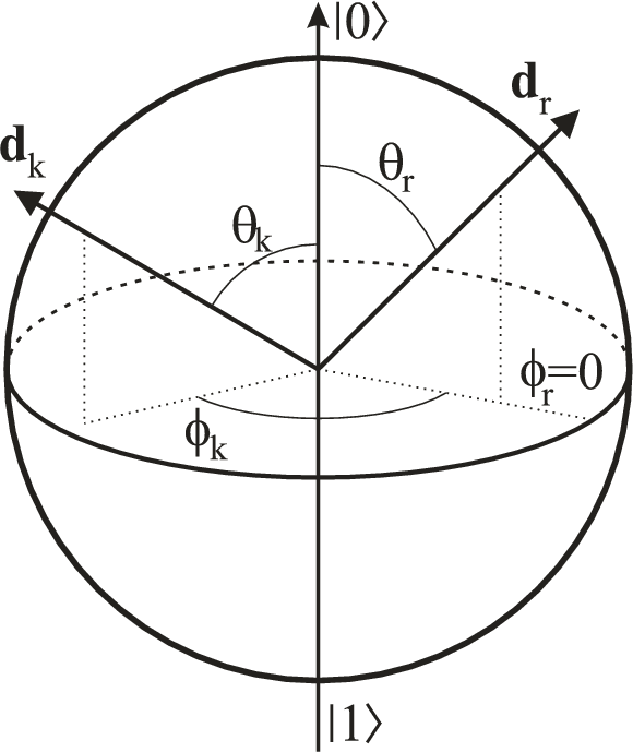
(a)

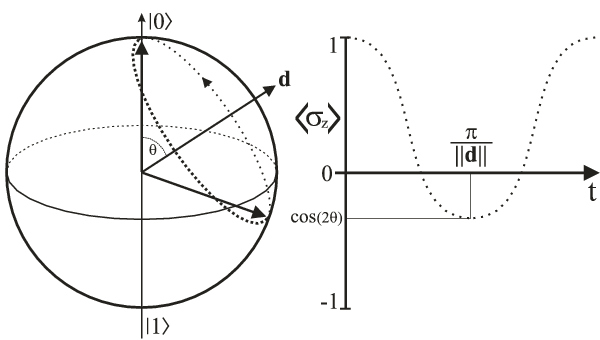
(b)

Figure 4: Bloch sphere representation of dynamics. (a) Arrangement of rotation axes ${\bf d}_{k}$ with respect to reference rotation axis ${\bf d}_{r}$. (b) The evolution of the vector ${\bf s}(t)$ with ${\bf s}_{0}=(0,0,1)^{T}$ about the axis ${\bf d}$, and the projection of ${\bf s}(t)$ onto the ${\bf z}$-axis.

To relate the Hamiltonian parameters to observable dynamics, it is instructive to visualize qubit states and their evolution on the Bloch sphere. If we define ${\bf s}=(s_{x},s_{y},s_{z})^{T}$ with $s_{k}=\Tr(\hat{\rho}\hat{\sigma}_{k})$ for $k\in\{x,y,z\}$ then it is easy to check that there is a one-to-one correspondence between density operators $\hat{\rho}$ and points ${\bf s}$ inside the closed unit Ball in ${{\rm I}\kern-1.60004pt{\rm R}}^{3}$. Furthermore, the evolution of $\rho(t)$ under the (constant) Hamiltonian (12) corresponds to a rotation of ${\bf s}(t)$ about the (unit) axis $\hat{{\bf d}}=(\sin\theta\cos\phi,\sin\theta\sin\phi,\cos\theta)^{T}$ with angular velocity $\omega$ as illustrated in Fig. 4. The figure also shows that we can determine the angle $\theta$ and angular frequency $\|{\bf d}\|=\omega$ from the projection of ${\bf s}(t)$ under the rotation about the axis ${\bf d}$ onto the ${\bf z}$-axis. As the figure shows, given $z(t)$, we can in principle extract $\omega$ and $\theta$ from the first minimum $(t_{0},z_{0})$ of $z(t)$, although in practice it is usually preferable to use Fourier analysis or harmonic inversion techniques. $z(t)$, being the expectation value $\langle A(t)\rangle=\Tr[\hat{\sigma}_{z}\rho(t)]$ of the observable $\hat{A}=\hat{\sigma}_{z}$ in the state $\hat{\rho}(t)$, can be obtained experimentally as follows PRA69n050306 :

1. Initialize: Measure and record outcome $\lambda_{a}=\pm 1$ $\Rightarrow$ system in state $\lambda_{a}{\bf s}_{0}=\lambda_{a}(0,0,1)^{T}$.

2. Evolve: Let the system evolve for time $t$ under the control settings ${\bf f}$ $\Rightarrow$ system now in state $\lambda_{a}{\bf s}(t)=\lambda_{a}(x(t),y(t),z(t))^{T}$ with

   $$z(t)=\cos^{2}\theta+\sin^{2}\theta\cos(\omega t).$$ (13)

3. Measure: Repeat measurement and record outcome $\lambda_{b}=\pm 1$ $\Rightarrow$ system now in state $\lambda_{b}{\bf s}_{0}$.

4. Repeat: steps (i)–(iii) $N_{e}$ times.

Let $N_{a,b}$ be the number of times the the initial measurement produced outcome $\lambda_{a}$ and the final measurement produced outcome $\lambda_{b}$. Then there are four possible combinations of outcomes $N_{0,0}$, $N_{0,1}$, $N_{1,0}$ and $N_{1,1}$, which must add to the total number of experiments $N_{e}$. The number of experiments that started in the state $|0\rangle$ [or ${\bf s}_{0}=(0,0,1)^{T}$] is $N_{e}^{\prime}=N_{0,0}+N_{0,1}$, and the fraction of experiments for which the second measurement yields $\lambda_{0}$ conditioned on the system starting in the state $|0\rangle$ is $N_{0,0}/N_{e}^{\prime}$. Thus the ensemble average of $\hat{A}=\hat{\sigma}_{z}$ at time $t$, assuming we started in the state $|0\rangle$, is

$$\lambda_{0}\frac{N_{0,0}}{N_{e}^{\prime}}+\lambda_{1}\frac{N_{0,1}}{N_{e}^{\prime}}=\frac{\lambda_{0}N_{0,0}+\lambda_{1}N_{0,1}}{N_{0,0}+N_{0,1}},$$ (14)

and for $N_{e}\to\infty$ this relative frequency should approach the true expectation value of $z(t)$ assuming $z(0)=1$. Thus, we can in principle determine $z(t)$ to arbitrary accuracy by choosing $N_{e}$ large enough. By repeating the experiments for different evolution times $t_{k}$, e.g., using a stroboscopic mapping approach (see Fig. 5), we can determine $z(t)$ as a function of $t$, from which we can extract $\omega=\omega_{{\bf f}}$ and $\theta=\theta_{{\bf f}}$ as discussed. For instance, noting that $z(t)=2p_{0}(t)-1$, Fig. 3 shows that the 1st order Fourier peak $F(\omega)$ of $z(t)$ in this example is $F(\omega)\approx 2\times 0.2468=0.4935$ for $\omega\approx 2$ and thus comparison with Eq. (13) shows that $\sin^{2}\theta=2\Re[F(\omega)]$, or equivalently, $\theta\approx 1.4566$. These values are reasonably good estimates for the real values $\omega=2.0086$ and $\theta=-1.4780$, except for the sign of $\theta$, or the orientation of the rotation axis, which we cannot determine from the given data, as these rotations have identical projections onto the $z$-axis. This is reflected in Eq. (13) by the fact that both coefficients $\cos^{2}\theta$ and $\sin^{2}\theta$ contain squares. In principle, we can determine the parameters $\omega$ and $\theta$ to arbitrary accuracy using this approach based on regular sampling and Fourier analysis PRA71n062312 , although the total number of experiments can become prohibitively large. An alternative that merits further investigation is the use of adaptive sampling techniques to reduce the total number of experiments necessary.

4.2 Relative angles between rotation axes

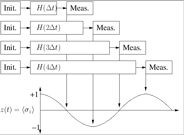
Figure 5: Stroboscopic mapping of coherent oscillations with projective measurements. After initialization through measurement, the system is allowed to evolve for fixed times under the influence of the controls before a second measurement is taken. The experiments are repeated to determine the expectation value of the observable at each time.

Having determined the parameters $\omega_{{\bf f}}$ and $\theta_{{\bf f}}$ for a particular control setting ${\bf f}$ and chosen a suitable reference Hamiltonian $\hat{H}_{\rm ref}$ with $\phi_{\rm ref}=0$, to complete the characterization of $\hat{H}_{{\bf f}}\neq\hat{H}_{\rm ref}$, we must determine the horizontal angle $\phi_{{\bf f}}$. The reference Hamiltonian $\hat{H}_{\rm ref}$ must not commute with the measured observable $\hat{A}$, or equivalently the angle $\theta_{\rm ref}$ between the rotation axis ${\bf d}_{\rm ref}$ and the ${\bf z}$-axis must be nonzero. Ideally ${\bf d}_{\rm ref}$ should be as close to orthogonal to the ${\bf z}$-axis as possible. Assuming $\theta_{\rm ref}\in(\pi/4,\pi/2]$, and $\omega_{{\bf f}}$ and $\theta_{{\bf f}}$ are known, we can determine the angles $\phi_{{\bf f}}$ by performing the following experiments PRA69n050306 :

1. Initialize: Measure and record outcome $\lambda_{a}=\pm 1$ $\Rightarrow$ system in state $\lambda_{a}{\bf s}_{0}=\lambda_{a}(0,0,1)^{T}$.

2. Prepare: Rotate around reference axis ${\bf d}_{\rm ref}$ by angle $\alpha_{0}=\arccos(\frac{1-x}{1+x})$, $x=-\cos(2\theta_{\rm ref})$ $\Rightarrow$ system in new state $\lambda_{a}{\bf s}_{1}=\lambda_{a}(\cos\beta,\sin\beta,0)^{T}$ with $\beta=\arctan(-\sqrt{2x})/\cos\theta_{\rm ref}$.

3. Evolve: Let the system evolve for time $t$ under the control settings ${\bf f}$ $\Rightarrow$ system in new state $\lambda_{a}{\bf s}(t)=\lambda_{a}(x(t),y(t),z(t))^{T}$ with

   $$z(t) =c[1-\cos(\omega_{{\bf f}}t)]+d\sin(\omega_{{\bf f}}t)$$ (15a)

   $$c =\sin\theta_{{\bf f}}\cos\theta_{{\bf f}}\cos(\phi_{{\bf f}}-\beta)$$ (15b)

   $$d =\sin\theta_{{\bf f}}\sin(\phi_{{\bf f}}-\beta).$$ (15c)

4. Measure: Repeat measurement and record outcome $\lambda_{b}=\pm 1$ $\Rightarrow$ system in new state $\lambda_{b}{\bf s}_{0}$.

5. Repeat: steps (i)–(iv) $N_{e}$ times.

As before, if $N_{a,b}$ is the number of times the initial measurement produced outcome $\lambda_{a}$ and the final measurement produced outcome $\lambda_{b}$ then we have

$$z(t)\approx\frac{\lambda_{0}N_{0,0}+\lambda_{1}N_{0,1}}{N_{0,0}+N_{0,1}}$$

for sufficiently large $N_{e}$, thus allowing us to determine $z(t)$ experimentally. Since $\theta_{{\bf f}}$, $\omega_{{\bf f}}$ and $\beta$ are known from the $\theta,\omega$ characterization step, Eq. (15) allows us to determine $\phi_{{\bf f}}$ via the coefficients $c$ and $d$, which can be determined in principle either through curve fitting or by taking the Fourier transform of $z(t)$ and noting that $c$ and $d$ correspond to the real and imaginary part of the 0th and 1st order Fourier peaks.

As a specific example, assume we have two Hamiltonians $\hat{H}_{1}$ and $\hat{H}_{2}$ and we have already determined $\omega_{1}=1$, $\theta_{1}=\frac{\pi}{4}$, and $\omega_{2}=1.2$, $\theta_{2}=\frac{\pi}{6}$. We choose $\hat{H}_{1}$ as reference Hamiltonian and note that a rotation about $\hat{H}_{1}$ by $\alpha=\pi$ maps the state ${\bf s}_{0}=(0,0,1)^{T}$ to ${\bf s}_{1}=(1,0,0)^{T}$. We then let state ${\bf s}_{1}$ evolve for different length of time $t$ under Hamiltonian $\hat{H}_{2}$, and determine the projection $z(t)$. This will produce a measured $z$-trace as shown in Fig. 6. Eq. (15) shows that in theory the height of the real part of the 0th and 1st order Fourier peaks should be the same except for the sign, but the graph clearly shows that this is not the case for our noisy (simulated) experimental data. In fact, the 1st order peaks around $\pm\omega_{{\bf f}}$ are significantly broadened, while the $0$-peak is very narrow. This suggests that we are likely to obtain the best estimate for $\phi$ by setting $c=\mbox{\rm FT}[z](0)$ and $\phi_{{\bf f}}=\arccos[c/(\sin\theta_{{\bf f}}\cos\theta_{{\bf f}})]+\beta$, where $\beta=0$ in our case. Indeed, this yields an estimate of $\phi_{{\bf f}}=0.2518\pi$, which is very close to actual value $\pi/4$ used in the simulation. Note that using the 1st order Fourier peaks gives far less accurate results due to the significant broadening of the peaks. This can be reduced using phase matching conditions and other tricks PRA71n062312 , but in this case simply using only the 0-peak is sufficient to get a good estimate.

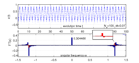
Figure 6: Determination of relative horizontal angle between two Hamiltonians. Measured projection $z(t)$ of ${\bf s}_{1}(t)$ onto the $z$-axis and corresponding Fourier spectrum. Blue/red bars indicate the cosine/sine coefficients, i.e., real/imaginary parts of the Fourier transform, respectively.

4.3 Functional dependence on control settings

In some settings it is sufficient to characterize the Hamiltonians $\hat{H}_{{\bf f}}$ for a discrete, finite set of controls $\{{\bf f}^{(k)}\}$. This would be the case for bang-bang-type control schemes that require only switching between a finite set of control Hamiltonians. In other cases, in particular when continuously varying fields are to be applied, we would also like to know the functional dependence of the Hamiltonian on the control fields, e.g., whether we can assume a control-linear model as in (4), or if there are non-linear or crosstalk effects, etc. Although characterizing the control dependence of the Hamiltonian is a non-trivial problem, given sufficiently many $\hat{H}_{{\bf f}}$ data points, it is possible to test the quality of fit of a particular model using statistical means. For instance, suppose we have characterized the Hamiltonians $\hat{H}_{{\bf f}}$ for ${\bf f}\in\{{\bf f}^{(k)}\}$. Let ${\bf d}_{k}$ be the corresponding vectors in ${{\rm I}\kern-1.60004pt{\rm R}}^{3}$ as defined above, and let $f_{m}^{(k)}$ be the $m$th component of the control vector ${\bf f}^{(k)}$. We can find the best-fitting linear model by finding vectors $\tilde{{\bf d}}_{m}\in{{\rm I}\kern-1.60004pt{\rm R}}^{3}$, $m=0,\ldots,M$, where $M$ is the number of independent control variables, that minimize the norm of the residuals $\Delta=\sqrt{\sum_{k}\|{\bf r}_{k}\|_{2}^{2}}$ where

$${\bf r}_{k}=\tilde{{\bf d}}_{0}+\sum_{m=1}^{M}f_{m}^{(k)}\tilde{{\bf d}}_{m}-{\bf d}_{k}.$$ (16)

The norm of the residuals $\Delta$ then gives an indication of the quality of fit of a linear dependence model, and allows us to compare the quality of fit for different models.

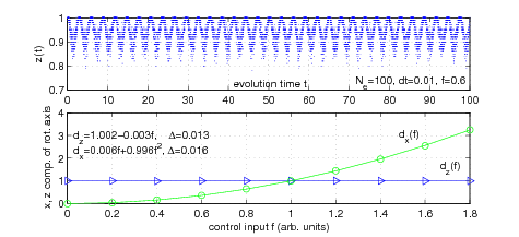
Figure 7: Determination of functional dependence of $\hat{H}_{{\bf f}}$ on control input ${\bf f}$. The bottom graph shows the estimated values for $d_{x}^{(k)}$ and $d_{z}^{(k)}$ (circles and triangles, respectively) as well as the actual functional dependence in the model (solid lines). The top graph shows a typical $z(t)$ trace obtained by averaging over $N_{e}=100$ simulated experiments for each time $t_{k}=0.01k$. The effects of finite sampling and projection noise are clearly visible for this trace. Nonetheless, the predicted functional dependence of $\hat{H}_{f}$ on the control input $f$ is in good agreement with the actual dependence in the model.

As an example, consider a Hamiltonian $\hat{H}_{{\bf f}}$ depending on a one-dimensional control input ${\bf f}=f$. To characterize the functional dependence of $\hat{H}_{f}$ on $f$, we choose a finite set of control settings $f_{k}=0.2(k-1)$ for $k=1,\ldots,10$. We characterize first the rotation frequencies $\omega_{k}$ and declination angles $\theta_{k}$ for each $f_{k}$, and then the relative angles $\phi_{k}$ as discussed above. From these, we calculate the components $d_{x}^{(k)}$, $d_{y}^{(k)}$ and $d_{z}^{(k)}$ of the Hamiltonian according to Eq. (12), and plot them versus $f$ as shown in Fig. 7. Specifically, in our case we find $\phi_{k}\approx 0$ and hence $d_{y}\equiv 0$, $d_{z}$ appears to be constant and $d_{x}$ exhibits a quadratic dependence on the control $f$. A least square fit of the data using a linear and quadratic fitting function, respectively, yields $d_{z}(f)=1.002-0.003\,f$ and $d_{x}(t)=0.006f+0.996f^{2}$, which is in very good agreement with the actual functional dependence in the model $d_{z}(f)=1$ and $d_{x}(f)=f^{2}$ despite the fact that the simulated data appears very noisy and the $\theta$ and $\omega$ estimates did not employ tuning such as phase matching to further improve the accuracy.

4.4 Characterization in the presence of decoherence

The protocols for Hamiltonian identification above are sufficient if dissipative effects are small on the timescales for coherent control, i.e., if the system and environment coupling is much weaker than the system-control interaction. If the coupling between the system and its environment is stronger then dissipative effects must be directly incorporated into the characterization protocols.

Assuming Markovian decoherence of the form (2), it is easy to show that for $N=2$, we have $\hat{A}_{k}=\hat{U}\hat{\sigma}_{k}\hat{U}^{\dagger}$, where $\hat{\sigma}_{k}$ are the elementary relaxation operators $\{\hat{\sigma}_{-},\hat{\sigma}_{+},\frac{1}{2}\hat{\sigma}_{z}\}$ defined in terms of the Pauli matrices $\hat{\sigma}_{\pm}=\frac{1}{2}(\hat{\sigma}_{x}\mp\rmi\hat{\sigma}_{y})$, and $\hat{U}$ is some unitary operator in ${\text{\liouvop SU}}(2)$ that defines a preferred decoherence basis. The operator $\hat{\sigma}_{z}$ is usually associated with pure decoherence (pure dephasing) while the raising and lowering operators $\hat{\sigma}_{\pm}$ are associated with population relaxation from $|1\rangle$ to $|0\rangle$ and vice versa. Very often it is furthermore assumed that $\hat{U}=\hat{I}$ is the identity, i.e., that the preferred basis for relaxation is the same as the measurement basis. Although this need not be the case, it is often a good approximation. The main effect of relaxation processes is to dampen the observed coherent oscillations $z(t)$ that result from the Hamiltonian dynamics, and try to force the system ‘asymptotically’ into a ‘steady’ state. This effect manifests itself in Lorentzian broadening of the peaks in the oscillation spectrum, which can be used for characterization purposes.

For example, Fig. 8 shows significantly damped oscillations as a result of relaxation. The fact that the oscillations decay to $z_{\infty}=0$ suggests either pure dephasing, or a symmetric relaxation process with $\Gamma_{+}=\Gamma_{-}$, i.e., equal probability of relaxation from state $|0\rangle$ to $|1\rangle$ and vice versa, or a combination of both. Since symmetric relaxation and pure dephasing have very similar signatures, it can be difficult to distinguish these processes from the oscillation trace alone. However, if there exists a control ${\bf f}$ such that $\hat{H}_{{\bf f}}\propto\hat{\sigma}_{z}$, which corresponds to a rotation about the ${\bf z}$ (or measurement) axis, then we can in principle distinguish the two processes by initializing the system repeatedly in either state $|0\rangle$ or $|1\rangle$ and letting the system evolve under $\hat{H}_{{\bf f}}$ for various periods of time before measuring again. If the decoherence process is pure dephasing then the system will remain in the initial state, while we expect to observe random jumps (with equal probability) for symmetric relaxation. Assuming this preliminary characterization step suggests that the damping in the figure is due to pure dephasing, we can then extract information about the rotation frequency $\omega_{0}$ and dephasing rate $\Gamma$ by fitting a Lorentzian envelope function

$$L_{\omega_{0},\Gamma}(\omega)=\frac{\Gamma}{(\omega-\omega_{0})^{2}+\Gamma^{2}}$$ (17)

to the first-order peak in the Fourier spectrum as shown in the figure. In our example, using a simple least-squares minimization yields estimated values for both $\omega_{0}$ and $\Gamma$ that are close to the actual values used in the simulated experiment. This approach can be generalized for more complicated relaxation processes PRA73n062333 . Alternatively, if we can characterize the Hamiltonian dynamics sufficiently to be able to initialize the system in non-measurement basis states and simulate readout in different bases, then generalized Lindblad operators can be estimated using repeated process tomography PRA67n042322 .

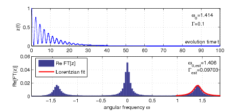
Figure 8: Characterization in the presence of decoherence. The observed damped oscillations due to pure dephasing (top) result in Lorentzian broadening of the Fourier peaks, which can be exploited to obtain (good) estimates for the rotation frequency $\omega_{0}$ and decoherence rate $\Gamma$.

5 Discussion of generalizations and conclusions

We have described some basic tools and techniques for characterizing the extent to which the dynamics of a certain system is confined to a low-dimensional subspace of a potentially large Hilbert space, as well as for identifying both Hamiltonian and decoherence parameters experimentally, with emphasis on protocols that are realistic even in the presence of limited direct readout and control capabilities.

Although the explicit schemes presented focused on qubit-like systems, the same basic ideas can be applied to higher-dimensional systems. However, the number of Hamiltonian and decoherence parameters to be determined for higher-dimensional system makes finding explicit protocols for complete characterization quite challenging. The qubit characterization protocols show that identifying the relative angles between several control Hamiltonians requires a two-stage process and more complicated two-step experiments (initialization in non-measurement basis state followed by controlled evolution) than identifying the rotation frequency and declination angle for a single Hamiltonian. As the dimension of the system increases more parameters are necessary to fully characterize the Hamiltonians, leading to more complex multi-stage characterization protocols.

Another problem is that the number of experiments required to implement such schemes may become prohibitively large for parameter estimation based on spectroscopic analysis. One of the most promising strategies to avoid this problem is the development of efficient adaptive characterization schemes—as opposed to protocols based on regular sampling— to minimize the number of measurements / experiments required. For systems composed of separate smaller units such as multi-qubit systems, boot-strapping approaches to characterization may also provide a fruitful alternative. For example, assuming we have separately characterized individual qubits using qubit identification protocols and therefore have full local control, we can reduce the problem of two-qubit identification in principle to identifying the interaction Hamiltonian. For two-qubit systems with local control and a fully non-local interaction Hamiltonian this can be achieved using entanglement mapping or concurrence spectroscopy devitt:052317 ; JPA39p14649 .

SGS acknowledges funding from an EPSRC Advanced Research Fellowship and support from Hitachi and the EPSRC QIP IRC. DKLO is supported by a SUPA fellowship. SJD acknowledges support from MEXT.

References

- (1) Nielsen M A and Chuang I L 2000 Quantum Computation and Quantum Information (Cambridge, UK: Cambridge University Press)
- (2) Gorman J, Hasko D G and Williams D A 2005 Phys. Rev. Lett. 95 090502
- (3) Lindblad G 1976 Comm. Math. Phys. 48 119–130
- (4) Gorini V, Kossakowski A and Sudarshan E C G 1976 J. Math. Phys. 17 821–825
- (5) Devoret M H and Schoelkopf R J 2000 Nature 406 1039
- (6) Chuang I L and Nielson M A 1997 J. Mod. Opt. 44 2455
- (7) Poyatos J F, Cirac J I and Zoller P 1997 Phys. Rev. Lett. 78 0390
- (8) Leung D W 2003 J. Math. Phys. 44 0528
- (9) Thew R T, Nemoto K, White A G and Munro W J 2002 Phys. Rev. A 66 012303
- (10) Kosut R, Walmsley I A and Rabitz H 2004 Optimal experiment design for quantum state and progress tomography and Hamiltonian parameter estimation quant-ph/0411093
- (11) Devitt S J, Schirmer S G, Oi D K L, Cole J H and Hollenberg L C L 2007 New J. Physics 7 384
- (12) Schirmer S G, Kolli A and Oi D K L 2004 Phys. Rev. A 69 050603(R)
- (13) Cole J H, Schirmer S G, Greentree A D, Wellard C J, Oi D K L and Hollenberg L C L 2005 Phys. Rev. A 71 062312
- (14) Cole J H, Greentree A D, Oi D K L, Schirmer S G, Wellard C J and Hollenberg L C L 2006 Phys. Rev. A 73 062333
- (15) Boulant N, Havel T F, Pravia M A and Cory D G 2003 Phys. Rev. A 67 042322
- (16) Devitt S J, Cole J H and Hollenberg L C L 2006 Phys. Rev. A 73 052317
- (17) Cole J, Devitt S and Hollenberg L 2006 J. Phys. A 39 14649–14658