Chandra HETG line spectroscopy of the Non-magnetic Cataclysmic Variable SS Cyg

Abstract

We present Chandra HETG observations of SS Cygni in quiescence and outburst. The spectra are characterized by He-like and H-like ${\rm K\alpha}$ emission lines from O to Fe, as well as L-shell emission lines from Fe. In quiescence, the spectra are dominated by the H-like ${\rm K\alpha}$ lines, whereas in outburst the He-like lines are as intense as the H-like lines. In outburst, the H-like ${\rm K\alpha}$ lines from O to Si are broad, with widths of 4–14$\ {\rm eV}$ in Gaussian $\sigma$ (1800–2300$\ {\rm km\ s^{-1}}$). The large line widths, together with line profiles, indicate that the line-emitting plasma is associated with the Keplerian disk and still retains the azimuthal bulk motion. In quiescence, the emission lines are narrower, with a Gaussian $\sigma$ of 1–3$\ {\rm eV}$ (420–620$\ {\rm km\ s^{-1}}$). A slightly larger velocity for lighter elements suggests that the lines in quiescence are emitted from an ionizing plasma at the entrance of the boundary layer, where the bulk motion of the optically thick accretion disk is converted into heat due to friction. Using the line intensity ratio of He-like and H-like ${\rm K\alpha}$ lines for each element, we have also investigated the temperature distribution in the boundary layer both in quiescence and outburst. The distribution of SS Cyg is found to be consistent with other dwarf novae investigated systematically with ASCA data.

1 Introduction

A dwarf nova is a close binary system consisting of a weakly magnetized white dwarf and a low-mass companion filling its Roche lobe and is characterized by frequent and large-amplitude optical outbursts. Mass accretion from the companion occurs via an optically thick disk extending down close to the white dwarf, and a so-called boundary layer is formed between the white dwarf and the innermost edge of the accretion disk, where the accreting matter is braked due to strong friction and finally settles onto the white dwarf.

After a long debate since the 1970’s, it is now widely accepted that the optical outburst arises due to a thermoviscous instability in an outer region of the accretion disk. In quiescence, matter from the companion is accumulated in the disk because the hydrogen is neutral, and hence the disk viscosity is low. As matter accumulates and the temperature exceeds $\sim$10⁴ K, the viscosity increases due to hydrogen ionization, and matter rushes onto the white dwarf at a rate exceeding the supply rate from the companion. This latter state is the optical outburst (Smak, 1984; Cannizzo, 1993; Osaki, 1996; Lasota, 2001). In response to the phase transition of the outer disk, it is predicted that the physical state of the boundary layer changes significantly. In quiescence, the boundary layer is optically thin, because the mass accretion rate is low and the radiative cooling is inefficient. The temperature is as high as $10^{8}$ K, and the boundary layer is a hard X-ray emitter. In outburst, on the other hand, the boundary layer can remain optically thick just as for the outer region of the disk, because of efficient radiative cooling. Since its temperature is $\sim\!10^{5}$ K, it emits mainly in the EUV band (Pringle, 1977; Pringle & Savonije, 1979; Tylenda, 1981; Patterson & Raymond, 1985). The first observational suggestion to support this phase transition was obtained from a series of European X-ray Observatory Satellite (EXOSAT) observations (Jones & Watson, 1992) and was finally established by Wheatley et al. (2003).

Although the phase transition of the boundary layer is better understood than in the past, there still remain several unresolved issues. Although the boundary layer is believed to be optically thick in outburst, optically thin hard X-ray emission above 2 keV does not vanish completely (Nousek et al., 1994; Wheatley et al., 2003). Unlike the magnetic CVs in which the postshock accretion flow is essentially one-dimensional, the temperature distribution of the boundary layer plasma is not understood very well. The temperature distribution is probably tightly linked with the geometry of the boundary layer, for which we have no more than a rough sketch. In order to help resolve these issues, we analyzed Chandra HETG data of SS Cyg. Since SS Cyg is the brightest dwarf nova in X-rays, it has been observed with many X-ray astronomy satellites, such as EXOSAT, Ginga, the Rossi X-ray Timing Explorer (RXTE), the Advanced Satellite for Cosmology and Astrophysics (ASCA), Chandra, and Suzaku (Yoshida et al., 1992; Nousek et al., 1994; Done & Osborne, 1997; Wheatley et al., 2003; Mauche, 2004; Mauche et al., 2005; Ishida et al., 2007). Since the Chandra HETG has an advantageous energy resolution, we have attempted to approach these unresolved issues by means of spectroscopy of He-like and H-like ${\rm K\alpha}$ emission lines. We discuss the temperature distribution and the geometrical structure of the boundary layer based on our results. In § 2 we introduce the Chandra observations of SS Cyg in outburst and quiescence and present light curves and spectra. In § 3, the data analysis method and the results are presented. The results are discussed in § 4, and the conclusions are summarized in § 5.

2 Observations

2.1 Chandra data

The SS Cyg data analyzed in this paper were retrieved from the Chandra Data Archive maintained by the Smithonian Astrophysical Observatory. The data in quiescence were obtained between 10:28 UT on 2000 August 24 and 00:19 UT on August 25, with a total good time interval of 47.3 ks. The outburst data were obtained from 21:09 UT on 2000 September 14 to 14:15 UT on the following day, with a total good exposure time of 59.5 ks. Both Chandra observations employed the High Energy Transmission Grating (HETG) (Canizares et al., 2005), which allows us to carry out fine spectroscopy with energy resolution better than CCD resolution by roughly an order of magnitude. These data are analyzed also by Mukai et al. (2003), Mauche et al. (2005), and Rana et al. (2006). By referring to the light curve from the AAVSO home page, we know that the visual magnitude of SS Cyg during the quiescence observation was in the usual range, 11.5–12.5. It then went into a normal outburst around September 10. Hence the Chandra outburst observation was performed $\sim$4–5 days after the onset of the outburst ($\sim$3 days after the peak with $m_{V}\simeq 8.5$). The visual magnitude during the Chandra observation was $m_{V}$ = 9.1–9.7.

2.2 Light curves in quiescence and outburst

The HETG consists of two independent grating instruments: the Medium Energy Grating (MEG), which covers the 0.4–5.0 keV band with an energy resolution $E/\Delta E$ of $\sim$200 at 2.0 keV, and the High Energy Grating (HEG), which covers the 0.8–10.0 keV band with $E/\Delta E\simeq$ 200 at 6.0 keV. In analyzing the data, we used the CIAO software (Version 3.2) and CALDB (Version 3.1.0) provided by the Chandra data center. Figure 1 shows the HETG light curves of SS Cyg in quiescence and in outburst. These light curves were made by summing up the positive and negative first-order photons in the above energy bands with a 512 s bin width using the thread dmextract. Backgrounds are not subtracted. The count rate of the MEG was ${\rm 2.90\pm 0.47\ c\ s^{-2}}$ and ${\rm 1.00\pm 0.07\ c\ s^{-1}}$ in quiescence and outburst, respectively. That of the HEG was, on the other hand, ${\rm 1.29\pm 0.22\ c\ s^{-1}}$ and ${\rm 0.44\pm 0.04\ c\ s^{-1}}$ in quiescence and outburst. The intensity of SS Cyg in outburst is less than that in quiescence by a factor of 3 on average and is less variable. The weaker X-ray intensity during optical outburst is associated with the optically thin-to-thick transition of the boundary layer when the mass transfer rate in the outer disk exceeds a critical value (Pringle, 1977; Pringle & Savonije, 1979; Tylenda, 1981; Patterson & Raymond, 1985). Such events are detected by coordinated optical, EUV, and X-ray observations (Wheatley et al., 2003).

2.3 HETG spectra in quiescence and outburst

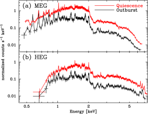
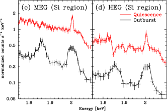
Figure 2: Spectra of SS Cyg in quiescence and outburst from (a) the MEG and (b) the HEG. Blow-up of (c) the MEG and (d) HEG spectra around the He-like and H-like Si ${\rm K\alpha}$ lines.

In Fig. 2 we show spectra of SS Cyg in quiescence and outburst from the MEG and the HEG separately. The spectrum files (PHA files) were extracted from the level 1 data, and the positive and negative orders were combined to enhance the signal-to-noise ratio. The MEG has a larger effective area in the lower energy range and has clearly detected ${\rm K\alpha}$ emission lines from O, Ne, Mg, and Si, while the HEG is advantageous at higher energies and has detected ${\rm K\alpha}$ lines from Fe. Simultaneous detection of the ${\rm K\alpha}$ emission lines from these elements indicates the existence of optically thin thermal plasma with a wide range of temperature distribution, both in quiescence and outburst. In quiescence, the spectra are dominated by the H-like lines, whereas in outburst, the He-like lines are as strong as the H-like lines. It is remarkable that, as demonstrated in Fig. 2(c) and (d), the emission lines in outburst are much broader than in quiescence. These characteristics are also pointed out by Mauche et al. (2005). The profiles of the H-like lines appear rectangular, rather than Gaussian-like.

3 Data analysis

As described in § 1, we aim to elucidate the nature of the boundary layer of SS Cyg in terms of ${\rm K\alpha}$ emission lines from abundant metals. We restrict ourselves to those from O up to Si, because the quantum efficiency of both the MEG and HEG abruptly drops by a factor of $\sim$5 at the iridium M edge $\sim$2.1 keV (Fig. 2), above which energy the line parameters are not very well constrained. Since the MEG has better sensitivity than the HEG in this energy band, we concentrate on the MEG spectra, except for evaluation of the H-like Si ${\rm K\alpha}$ line, for which we also utilize the HEG data (§ 3.3 and § 3.4).

3.1 Continuum

In analyzing emission lines, we first attempted to evaluate the continuum spectrum of the MEG in the 0.4–2.3 keV band. We masked energy bins, including the emission lines, and fitted the remaining spectrum with a bremsstrahlung model undergoing a uniform photoelectric absorption. Prior to the fitting process, the spectra were rebinned so that each energy bin includes at least 100 photons in quiescence and 50 photons in outburst, respectively. The fits to the quiescence and outburst spectra were marginally acceptable at the 90% confidence level ($\chi^{2}$ [dof] of 452.5 [441] and 300.7 [241], respectively), with temperatures of ${\rm 14.5^{+4.8}_{-3.5}}$ and ${\rm 4.3^{+1.9}_{-0.7}\ keV}$ and with $N_{\rm H}<0.3\times{\rm 10^{20}\ cm^{-2}}$ and ${\rm<1.1\times 10^{20}\ cm^{-2}}$, respectively. The fits were improved significantly when we adopted a partially covering absorber with $\chi^{2}$ (d.o.f.) of 404.3 (440) and 259.1 (240). The temperature of the thermal bremsstrahlung in quiescence and outburst is ${\rm 4.1^{+1.4}_{-0.9}\ keV}$ and ${\rm 1.6^{+1.5}_{-0.9}\ keV}$, which is covered with an absorber with $N_{H}=3.9^{+1.4}_{-0.9}\times 10^{19}\ {\rm cm^{-2}}$ and $4.9^{+1.5}_{-0.9}\times 10^{19}\ {\rm cm^{-2}}$ by ${\rm 57^{+10}_{-9}}$% and ${\rm 84^{+5}_{-7}}$%, respectively. Below we adopt the latter as the continuum model.

3.2 Emission lines

Given the continuum model, we retrieved all the energy channels and tried to evaluate the line parameters. We fixed all the continuum parameters at the best-fit values in § 3.1, except for the normalization, and added Gaussians to represent the H-like and He-like ${\rm K\alpha}$ lines of O, Ne, Mg, and Si. In fitting these Gaussians to the data, all the parameters were allowed to vary. Table 1 summarizes the best-fit parameters of the ${\rm K\alpha}$ lines thus obtained in quiescence and outburst, together with the ionization temperature obtained from the He-like and H-like line intensity ratio, which are plotted in Fig. 3.

It is clear that the obtained ionization temperatures of all ions in quiescence are systematically higher than those in outburst. They show a wide range depending on the element, from 0.3 to 2.0 keV in quiescence and from 0.2 to 1.2 keV in outburst. The emission lines seen in the 0.7–0.9$\ {\rm keV}$ bands are from L-shell Fe (mainly Ne-like), indicating the existence of a plasma component with a temperature of $\sim 4\times 10^{6}\ {\rm K}$ (Arnaud & Raymond, 1992). These facts unambiguously indicate that the plasma in the boundary layer has a significant temperature distribution. The differences in the line intensity ratio distribution, as well as in the line profiles, probably reflect a significant structural difference of the boundary layer between quiescence and outburst.

3.3 H-like line profile in outburst

Unlike the He-like ${\rm K\alpha}$ line, which is composed of the resonance, intercombination, and forbidden lines, as well as satellite lines, the intrinsic structure of the H-like ${\rm K\alpha}$ line is much simpler, consisting only of the following two resonance lines: ${}^{2}{\rm P}_{1/2}\rightarrow^{2}\!{\rm S}_{1/2}$ and ${}^{2}{\rm P}_{3/2}\rightarrow^{2}\!{\rm S}_{1/2}$. Moreover, their energy separation is only 2.0 eV for Si ($E=2003.9$ eV and 2005.9 eV, respectively) and is even smaller for the lighter elements. We can thus regard the H-like ${\rm K\alpha}$ lines of O, Ne, Mg, and Si as consisting of a single component for the HETG resolution, and their profile can be used to diagnose the geometry and the dynamical motion of the line-emitting plasma.

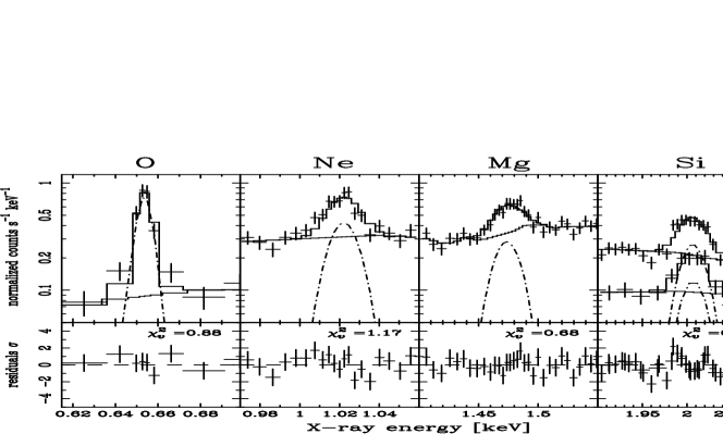
Figure 4: Results of a Gaussian fit to the MEG spectra of the H-like ${\rm K\alpha}$ lines. The HEG spectra are also used for the Si ${\rm K\alpha}$ line. The fits are acceptable at the 90% confidence level.

From Table 1, it is seen that all the H-like ${\rm K\alpha}$ lines are significantly broader in outburst than in quiescence (see also Fig. 2). Their widths are in the range 4–14$\ {\rm eV}$ in Gaussian $\sigma$, and corresponding velocities are 1800–2300$\ {\rm km\ s^{-1}}$. Their central energies are consistent with those in the laboratory. Their profiles, fitted with a broad Gaussian, are shown in Fig. 4. We then fixed $E_{\rm c}$ at the laboratory values, which are defined as the emissivity-weighted means of the Ly$\alpha$ doublet.

The abscissa axis covers an energy range of 10% of each line’s rest-frame energy. The best-fit parameters fitted with the broad Gaussian are summarized in table 2. Although all the fits are already acceptable at the 90% confidence level, the profile seems to change from a Gaussian for lighter elements to a somewhat rectangular structure for heavier elements.

The rectangular line profile is reminiscent of a homogeneously emitting thin spherical shell that is radially in- or outflowing (Hynes et al., 2002). Of these, an outflow associated with SS Cyg in outburst is detected as the disk wind by the Chandra LETG (Mauche, 2004). The wind is detected as blueshifted absorption lines with a velocity of 2500$\ {\rm km\ s^{-1}}$ due to intermediately ionized O through Fe, overlaid on a blackbody emission with a temperature of $250\pm 50$kK. Based on this fact, we infer that the observed H-like emission lines would also have been blueshifted, because the plasma below the accretion disk is invisible to us. We thus consider the radial outflow picture unlikely.

Compared with the outflow considered above, a radial inflow is more likely if the innermost part of the boundary layer becomes optically thin, as in quiescence. The plasma in the boundary layer then should take the form of a cooling flow for matter settling down onto the white dwarf. The temperature distribution demonstrated in § 3.2 is interpreted as a radial stratification in the cooling flow. The plasma emitting any given line can be treated as a geometrically thin spherical shell, since the emissivity of any ${\rm K\alpha}$ line is so sensitive to the plasma temperature.

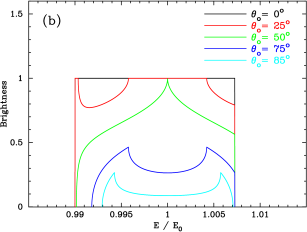
Figure 5: (a) Schematic view of the stratified shell model, and (b) an example of the line profiles. The adopted parameters are $i=$40^∘, $r_{\rm sh}/R_{\rm WD}=1.45$, and $v=3000\ {\rm km\ s^{-1}}$, and the line profiles are shown at opening angles $\theta_{\rm o}=$ 0^∘, 25^∘, 50^∘, 75^∘, and 85^∘.

In order to see whether the radial inflow interpretation is acceptable, we have constructed a model representing a profile of an emission line emanating from a geometrically thin uniform shell falling onto a white dwarf. The free parameters of the model are the radial velocity $v$, the radius of the shell $r_{\rm sh}$, the opening polar angle of the shell $\theta_{\rm o}$, the inclination angle of the orbital plane $i$, and the central energy of the emission line $E_{\rm c}$ (see Fig. 5a).

The white dwarf always hides the most blueshifted part of the shell, and the hidden fraction is determined solely by $r_{\rm sh}/R_{\rm WD}$, where $R_{\rm WD}$ is the white dwarf radius. In the case that the shell does not expand above the orbital plane enough to form a complete sphere, we introduce the polar opening angle $\theta_{\rm o}$ within which the plasma is absent. Some examples of the resultant line profiles are shown in Fig. 5(b). Hereafter we refer to this model as the stratified shell model.

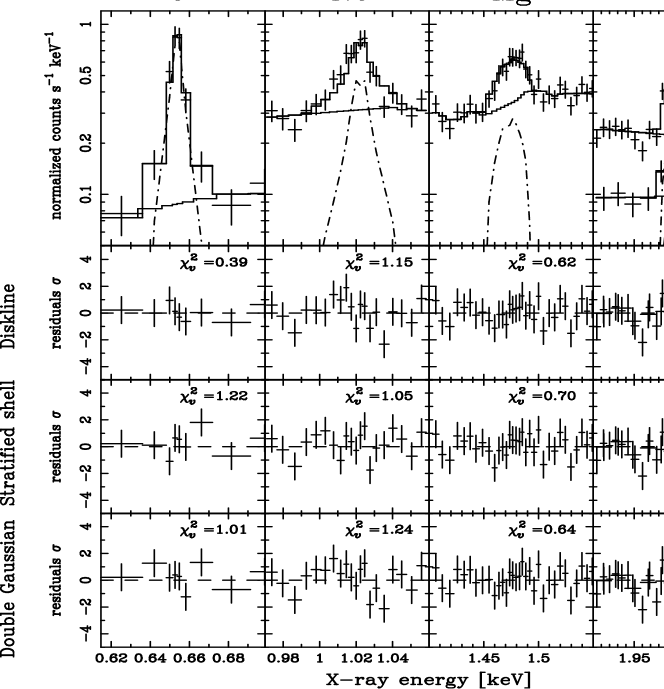
Figure 6: Results of the fits of (top), the stratified shell model (middle) the diskline model, and (bottom) the double-Gaussian model to the H-like ${\rm K\alpha}$ lines.

In fitting the model to the H-like ${\rm K\alpha}$ lines, we fixed $i$ at 40^∘, following the measurement of Shafter (1983). We also fixed $E_{\rm c}$ at the laboratory values. The best-fit parameters of the lines with the stratified shell model are summarized in table 3 and shown in Fig. 6. As expected, the fitting to the H-like Si ${\rm K\alpha}$ line is improved significantly, because the model can represent the shoulders of the profile appropriately. The fitting to Mg is, however, not improved significantly and that to Ne and O became poorer than the Gaussian fit. The radial velocity $v$ of all the elements is in the range 3400–4500 km s^-1 and does not show any sign of slowing down from the Si shell (higher $T$) to the O shell (lower $T$).

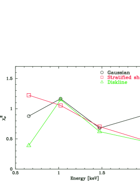
Figure 7: $\chi^{2}_{\nu}$ values of the fits to the O through Si lines with the single-Gaussian model, the stratified shell model, and the diskline mode.

Finally, we have tried the diskline model in XSPEC (Arnaud, 1996) to see whether the profile of the H-like ${\rm K\alpha}$ lines can be explained by a bulk azimuthal motion of the plasma around the white dwarf. The diskline model is intended to represent the emission line profile from a geometrically thin Keplerian disk irradiated by the central active galactic nucleus (AGN) via fluorescence, taking the gravitational redshift into account (Stella, 1990; Fabian et al., 1989). Hence, the parameters are the innermost radius of the disk $R_{\rm in}$ in units of the Schwarzschild radius and the radial power $q$ of the emissivity $\varepsilon(r)$ in the form $\varepsilon\propto r^{q}$. The results of the fits are summarized in table 4 and displayed in Fig. 6. The resultant $\chi^{2}_{\nu}$ values of the fits to the O through Si lines with the models introduced so far are shown in Fig. 7.

The diskline model can provide a comprehensive understanding to a variety of the H-like ${\rm K\alpha}$ line profiles from O (Gaussian) to Si (rectangular). On the basis of this result, we conclude that the profiles of the H-like ${\rm K\alpha}$ emission lines are best interpreted as due to azimuthal bulk motion of the optically thin thermal plasma.

3.4 Bulk motion of the plasma in outburst

As demonstrated in § 3.3, the nonrelativistic diskline model is successfully fitted to the H-like ${\rm K\alpha}$ lines from O to Si in outburst. This implies that the plasma has an azimuthal bulk motion. In order to evaluate this bulk motion, we hereafter fit the profiles of the H-like ${\rm K\alpha}$ lines with two Gaussians that represent the red- and blueshifted line components associated, respectively, with the receding and approaching parts of the plasma. The free parameters are the average energy of the two line components $E_{\rm c}$, the energy separation between them $E_{\rm sp}$, the energy widths $\sigma$, and the normalizations. Among these, $E_{\rm sp}$ is a measure of the absolute radial location of the annulus from which the corresponding H-like ${\rm K\alpha}$ line emanates, and $\sigma$ represents the geometrical width of the annulus. For simplicity, we set the $\sigma$ values, and the normalizations of the red- and blueshifted components are constrained to be common.

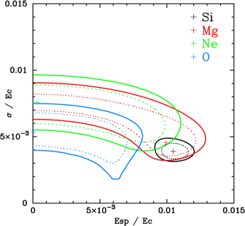
Figure 9: The 90% and 99% confidence contours (dotted and continuous lines, respectively) between the line separation energy $E_{\rm sp}$ and the line width $\sigma$ in the double-Gaussian model for the H-like ${\rm K\alpha}$ lines from O to Si. $E_{\rm sp}$ decreases from Si to O, and the 90% confidence contour of Si is isolated from that of O.

The results of the fits are summarized in Table 5 and shown in Fig. 6 and 8, with $\sigma$ and $E_{\rm sp}$ being normalized by $E_{\rm c}$. In addition, we draw confidence contours between $E_{\rm sp}$ and $\sigma$ in Fig. 9, since they may couple with each other.

From Fig. 8 and 9, $E_{\rm sp}$ is found to be smaller for lighter elements, and the 90% confidence contours of O and Si are separated, while $\sigma$ does not show any difference among the elements. In Table 5, the rotational velocity $v$ calculated from $E_{\rm sp}$ with $v=(E_{\rm sp}/2E_{\rm c})\,c$ is also listed. The rotational velocity of Si is $\sim$1500 km s^-1, whereas that of O is only $\sim$10 km s^-1.

4 Discussion

4.1 Geometry of line-emitting plasma in outburst

In § 3.3 and § 3.4, we have demonstrated that the profiles of H-like ${\rm K\alpha}$ lines from O to Si can be explained with the azimuthal bulk motion model (the diskline model), rather than the radial inflow model (the stratified shell model) on the basis of fit statistics, and we have obtained the bulk motion parameters with the double-Gaussian model. Besides the statistics, the high radial velocities of $v=$ 3400–4500 km s^-1 (table 3) are problematic for the stratified shell model. Since the ionization temperature of O in outburst is only $\sim$200 eV, its thermal velocity is as small as $\langle v_{\rm th}\rangle=\sqrt{3kT/m_{\rm O}}\simeq$350 km s^-1. Hence the plasma flow is highly supersonic, thereby forming a standing shock wave whose temperature $kT_{\rm s}=(3/16)\mu m_{\rm H}v^{2}$ is as high as 14–24 keV. However, no such high temperature component is detected. The Suzaku observations in outburst, for example, constrain the maximum temperature of the plasma to be $kT_{\rm max}{\rm=8.4\pm 1.0~{}keV}$ (Ishida et al., 2007).

These results indicate that the bulk motion in the optically thin thermal plasma in outburst is azimuthal rather than radial. Although the errors are somewhat large, the lighter elements are likely to have smaller $E_{\rm sp}$ (Fig. 8 and 9). It is natural to expect that both the temperature and the azimuthal bulk velocity are gradually reduced as the plasma approaches the white dwarf, because it eventually settles down onto the white dwarf. The double-Gaussian model is consistent with this expectation in that the lighter elements, which have lower ionization temperature, have smaller $E_{\rm sp}$.

Since the boundary layer is believed to be optically thick in outburst, it has been unclear where the observed optically thin thermal X-ray emission emanates. Our analysis indicates that the optically thin thermal plasma also shows a bulk azimuthal motion whose velocity decreases as the plasma cools and approaches the white dwarf. We infer that the optically thin thermal plasma exists over the optically thick disk like an accretion disk corona in low-mass X-ray binaries, as sketched in Patterson & Raymond (1985).

4.2 Line emission site in quiescence

In § 2.3 we demonstrated that the emission lines in the quiescent spectra (Fig. 2) are significantly narrower than those in outburst. Nevertheless, the lines still have finite widths in the range 1–3 eV in Gaussian $\sigma$ for the H-like ${\rm K\alpha}$ lines (Table 1). They are as large as 1 part per $\sim\!\!10^{3}$ of the line energies $E_{\rm c}$, and if they are attributed to thermal motion, then the following holds:

$$\frac{\sigma}{E_{\rm c}}\;=\;\frac{1}{c}\sqrt{\frac{1}{3}\langle v_{\rm th}^{2}\rangle}\;=\;\frac{1}{c}\sqrt{\frac{kT}{m}}$$

where ${\langle v_{\rm th}^{2}\rangle}^{1/2}$ is the root mean square of the thermal velocity. Using the atomic mass number $A$, we obtain

$$kT\;=\;mc^{2}\,\left(\frac{\sigma}{E_{\rm c}}\right)^{2}\;=\;75\,\left(\frac{A}{20}\right)\,\left(\frac{\sigma}{\mbox{2 eV}}\right)^{2}\,\left(\frac{E_{\rm c}}{\mbox{1 keV}}\right)^{-2}\;\;\mbox{keV},$$ (1)

which is 64 keV for O and 51 keV for Si. These temperatures are incompatible with the detection of the H-like ${\rm K\alpha}$ emission lines, because they are emitted from a plasma with a temperature of $\lesssim 1$ keV (Mewe et al., 1985). Hence, the line broadening should originate from a bulk motion whose geometry is so symmetric that the line Doppler shift is observed as a line broadening, not as a line shift. One may consider an outflow such as is observed in the EUV to soft X-ray band in outburst (Mauche, 2004). However, the outflow is probably located farther out of the optically thin boundary layer, and most of the receding parts of the plasma are hidden by the accretion disk. In fact, the soft X-ray absorption lines originating from the outflow in outburst are blueshifted (Mauche, 2004).

We consider the observed ${\rm K\alpha}$ emission lines from O to Si as emanating from a transition region from the optically thick accretion disk to the optically thin boundary layer, where the Keplerian motion is gradually converted into thermal motion due to strong friction. The average line-of-sight velocity dispersion estimated from the observation is

$$\langle v\rangle\;=\;\frac{\sigma}{E_{\rm c}}\,c\;=\;6.0\times 10^{2}\,\left(\frac{\sigma}{\mbox{2 eV}}\right)\,\left(\frac{E_{\rm c}}{\mbox{1 keV}}\right)^{-1}\;\;{\rm km\;s^{-1}},$$ (2)

which is 620${}^{+130}_{-170}$, 530${}^{+100}_{-120}$, $460^{+220}_{-120}$, and 420$\pm 140$ km s^-1 for O, Ne, Mg, and Si, respectively. This is roughly one-tenth of the Keplerian velocity on the surface of the 1.2$M_{\odot}$ white dwarf ($\simeq$6300 km s^-1). Even considering the inclination angle of 40^∘ and the line-of-sight average of the azimuthal velocity, $(2/\pi)\sin 40^{\circ}$, we obtain the maximum possible line-of-sight velocity to be $\langle v\rangle_{\rm max}=$2600 km s^-1, which can cover the average velocity eq. (2) evaluated from the observed line width.

As in outburst, the line width in quiescence can be attributed to azimuthal motion. Unlike in outburst, however, where the emission lines can be interpreted as being emitted from a cooling plasma, we believe those in quiescence are created in the heating process at the entrance to the optically thin boundary layer. In fact, although the statistical significance is not very high, the bulk velocity in quiescence estimated from the H-like ${\rm K\alpha}$ line widths seems to decrease from O to Si. It is likely that the plasma heating results from the conversion of the energy of bulk motion.

4.3 Temperature distribution

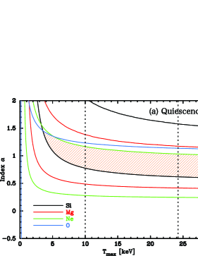
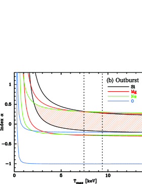
Figure 10: Areas allowed by the observed line intensity ratio of O, Ne, Mg, and Si in the plane of the two cemekl parameters $\alpha$ and $T_{max}$. The allowed areas are defined with the 90% confidence contours. Left and right panels are those for quiescence and outburst, respectively. Vertical dotted lines at $15.4^{+8.8}_{-5.4}$ and $8.4\pm 1.0$ keV are the values of $T_{\rm max}$ from Ishida et al. (2007) and Done & Osborne (1997), respectively.

In this section, we attempt to impose a constraint on the temperature distribution of the plasma in outburst and quiescence in terms of the intensity ratio of the He-like and H-like ${\rm K\alpha}$ emission lines. We simply assume that the differential emission measure $d(E\!M)$ is proportional to the power of the plasma temperature. In the following analysis, we adopt the spectral model cemekl, in which the temperature distribution is taken into account as $d(E\!M)\propto(T/T_{\rm max})^{\alpha}d(\log T)$ $\propto(T/T_{\rm max})^{\alpha-1}dT$, where $T_{\rm max}$ is the maximum temperature of the plasma. Hence, the exponent $\alpha$ obtained by a fit with this model is larger than the true weighting factor by 1 (Done & Osborne, 1997). In the framework of this model, the line intensity ratio is uniquely determined once $\alpha$ and $T_{\rm max}$ are given. Hence, we can conversely give a constraint on these two parameters with the line intensity ratios of O, Ne, Mg, and Si that we have obtained from the HETG data. The allowed parameter regions delineated by the 90% errors of the intensity ratios (Table 1) are shown in Fig. 10 with a different color for each element.

For all the elements, the contours become vertical, and $\alpha$ diverges as $T_{\rm max}$ decreases and approaches a certain value. This limiting $T_{\rm max}$ gives the temperature of the single-phase plasma that can reproduce the observed intensity ratio. On the contrary, the contour becomes horizontal in the high-$T_{\rm max}$ limit. Since the emissivity of atomic lines peaks at a finite temperature, the line ratio becomes insensitive to $T_{\rm max}$ and is determined solely by $\alpha$ if $T_{\rm max}$ becomes too high compared with the emissivity peak temperature. As shown in Fig. 10, there is a parameter region that can be shared by all elements (except for O in outburst). Taking into account the constraint $T_{\rm max}=8.4\pm 1.0$ keV for the outburst obtained from the Suzaku observation (Ishida et al., 2007), the common range of $\alpha$ is $-0.2$ to 0.3 in outburst. On the other hand, the maximum temperature is $15.4^{+8.8}_{-5.4}$ keV (Done & Osborne, 1997) in quiescence, which is significantly higher than in outburst, and the common range of $\alpha$ is found to be 0.6–1.2 in quiescence. This significant difference is probably the result of the geometrical difference of the optically thin boundary layer between quiescence and outburst (for example, see Patterson & Raymond (1985)).

We remark that only the index $\alpha$ of O in outburst is not common with the other elements. This is not unreasonable, in view of the shape of the cooling curve of an optically thin thermal plasma. Unlike the temperature region $T\gtrsim 2\times 10^{7}$ K, the slope of the plasma cooling curve shows a complicated change as a function of the temperature in the range $T\lesssim 10^{7}$ K (Gehrels & Williams, 1993). Since $\alpha$ of a given element reflects the slope of the cooling curve around the temperature at which the line emissivity of the element shows the peak, it is possible in principle that $\alpha$ is different for elements whose emissivity peak appears in the range $T\lesssim 10^{7}$ K.

The index of the temperature distribution $\alpha$ was systematically examined by Baskill et al. (2005) using the complete set of the ASCA nonmagnetic CV data. They found that $\alpha$ for the dwarf novae is in the range from 0.7 to 1.8 in quiescence (with a few exceptions) and $-$0.1 to 0.3 in outburst. The $\alpha$-values obtained from our analysis on SS Cyg in quiescence and outburst are both consistent with their results. Done & Osborne (1997) carried out the same analysis using the outburst and quiescence data of Ginga and ASCA. Although $\alpha$ in the quiescence Ginga data is not constrained very well ($2.9^{+\infty}_{-1.4}$), they derived $\alpha=0.43^{+0.41}_{-0.38}$ and $0.46^{+0.06}_{-0.05}$ for the normal and anomalous outbursts from the Ginga and ASCA data, respectively. The $\alpha$ of the anomalous outburst is outside the range of Baskill et al. (2005) and that of ours. The exponent $\alpha$ may possibly be different between the two types of the outburst and may depend on the intensity of the reflection component included in their modeling.

The temperature distribution in the postshock accretion column of a magnetic cataclysmic variables (mCVs) can be approximated as $T(z)\propto z^{2/5}$, where $z$ is the height from the white dwarf surface if the cooling mechanism is dominated by free-free emission (Frank et al., 2002). In this case, the cevmekl power $\alpha\simeq+0.5$ (Ishida et al., 1994), which lies between that in the quiescence and the outburst obtained from this work.

5 Conclusion

We have investigated the optically thin boundary layer of SS Cyg both in quiescence and in outburst by carrying out high resolution line spectroscopy with the Chandra HETG. The spectra contain He-like and H-like ${\rm K\alpha}$ emission lines from O to Fe, as well as L-shell emission lines from Fe, both in quiescence and outburst. However, the relative intensity of the He-like and H-like emission lines of a given element is significantly different; in outburst they are nearly equal, whereas in quiescence the H-like lines are much more intense than the He-like line. The ionization temperatures evaluated from the line intensity ratio of O, Mg, Ne, and Si are in the range 0.3–2.0 keV and 0.2–1.2 keV in quiescence and outburst, respectively.

The other remarkable difference of the line profiles between quiescence and outburst is in the line width. The H-like lines from O to Si in outburst are much broader, with widths of 4–14 eV in Gaussian $\sigma$ (1800–2300 km s^-1), and especially that of Si has a rectangular profile, rather than a Gaussian profile. Among a few possibilities, such as a homogeneously emitting thin spherical shell that is radially in- or outflowing, an azimuthal bulk motion, which can be mimicked by the diskline model, most naturally explains the observed line profile. The boundary layer is, however, believed to be optically thick all the way down to the white dwarf surface. We thus infer that the line-emitting plasma is located above the optically thick disk, like an accretion disk corona commonly seen in low-mass X-ray binaries. Since lighter elements tend to have a smaller bulk velocity, the observed line-emitting plasma in outburst is a cooling plasma.

Although less remarkable, the emission lines from O to Si in quiescence also have a finite line width with a Gaussian $\sigma$ of 1–3 eV (420–620 km s^-1). It is impossible to attribute the width to a thermal motion, because the resultant temperature becomes as high as $\gtrsim$50 keV. Since no red- or blueshift is detected for the line central energies, the radial in- or outflow is unlikely. The most natural origin of the bulk velocity is an azimuthal motion. A slightly larger velocity for lighter elements, contrary to outburst, suggests that the lines in quiescence are emitted in the heating process at the entrance to the boundary layer, where the bulk motion of the optically thick accretion disk is converted to thermal energy due to friction.

We have also investigated the temperature distribution in the boundary layer within a framework of the differential emission measure having a power-law distribution of the temperature as $(T/T_{\rm max})^{\alpha}$. From the line intensity ratio, the index $\alpha$ is constrained in the range from $-$0.2 to 0.3 in outburst and from 0.6 to 1.2 in quiescence. These values are consistent with those obtained from the previous systematic work of Baskill et al. (2005).

Table 1: Best-fit parameters of a Gaussian to the ${\rm K\alpha}$ lines and resultant ionization temperatures

	$E_{\rm c}$	$\sigma$	$I$	EW	$I_{\rm H}/I_{\rm He}$	$kT_{i}$
Ion	[keV]	[eV]	[${\rm 10^{-4}ph.\;cm^{-2}s^{-1}}$]	[eV]		[keV]
Quiescence
Si XIII	${\rm 1.8649^{+0.0030}_{-0.0058}}$	${\rm 6.16^{+5.55}_{-3.16}}$	${\rm 0.55^{+0.26}_{-0.27}}$	${\rm 2.9}$	…	…
Si XIV	${\rm 2.0052^{+0.0005}_{-0.0012}}$	${\rm 2.80^{+0.94}_{-0.95}}$	${\rm 1.53^{+0.24}_{-0.25}}$	${\rm 9.1}$	${\rm 2.79^{+1.44}_{-1.37}}$	${\rm 2.05^{+0.465}_{-0.53}}$
Mg XI	${\rm 1.3521^{+0.0024}_{-0.0020}}$	${\rm 4.17^{+3.83}_{-1.76}}$	${\rm 0.87^{+0.26}_{-0.40}}$	${\rm 2.6}$	…	…
Mg XII	${\rm 1.4720^{+0.0073}_{-0.0059}}$	${\rm 2.25^{+1.06}_{-0.61}}$	${\rm 1.54^{+0.35}_{-0.26}}$	${\rm 5.2}$	${\rm 1.78^{+0.90}_{-0.61}}$	${\rm 1.01^{+0.19}_{-0.15}}$
Ne IX	${\rm 0.9210^{+0.0017}_{-0.0009}}$	${\rm 2.15^{+1.21}_{-0.95}}$	${\rm 2.23^{+1.03}_{-0.76}}$	${\rm 3.5}$	…	…
Ne X	${\rm 1.0213^{+0.0411}_{-0.0003}}$	${\rm 1.81^{+0.33}_{-0.41}}$	${\rm 4.68^{+0.60}_{-0.76}}$	${\rm 8.7}$	${\rm 2.10^{+0.76}_{-1.03}}$	${\rm 0.62^{+0.08}_{-0.13}}$
O VII	${\rm 0.5702^{+0.0399}_{-0.0399}}$	${\rm 3.26^{+9.34}_{-1.63}}$	${\rm 7.27^{+5.28}_{-6.34}}$	${\rm 6.5}$	…	…
O VIII	${\rm 0.6533^{+0.0004}_{-0.0003}}$	${\rm 1.35^{+0.29}_{-0.36}}$	${\rm 13.78^{+2.27}_{-2.47}}$	${\rm 14.9}$	${\rm 1.90^{+1.42}_{-1.68}}$	${\rm 0.30^{+0.07}_{-0.15}}$
Outburst
Si XIII	${\rm 1.8603^{+0.0011}_{-0.0030}}$	${\rm 12.50^{+2.49}_{-1.00}}$	${\rm 4.62^{+0.71}_{-0.39}}$	${\rm 46.4}$	…	…
Si XIV	${\rm 2.0055^{+0.0023}_{-0.0023}}$	${\rm 13.88^{+2.04}_{-1.32}}$	${\rm 3.73^{+0.34}_{-0.61}}$	${\rm 45.4}$	${\rm 0.81^{+0.10}_{-0.18}}$	${\rm 1.22^{+0.053}_{-0.104}}$
Mg XI	${\rm 1.3494^{+0.0010}_{-0.0034}}$	${\rm 9.95^{+1.48}_{-1.66}}$	${\rm 5.52^{+0.57}_{-1.13}}$	${\rm 25.9}$	…	…
Mg XII	${\rm 1.4754^{+0.0014}_{-0.0031}}$	${\rm 10.24^{+1.82}_{-1.73}}$	${\rm 4.09^{+0.99}_{-0.45}}$	${\rm 23.4}$	${\rm 0.74^{+0.24}_{-0.11}}$	${\rm 0.74^{+0.07}_{-0.04}}$
Ne IX	${\rm 0.918^{+0.0014}_{-0.0011}}$	${\rm 5.78^{+1.22}_{-0.97}}$	${\rm 13.26^{+2.45}_{-2.04}}$	${\rm 23.2}$	…	…
Ne X	${\rm 1.0194^{+0.0016}_{-0.0014}}$	${\rm 7.89^{+1.48}_{-1.34}}$	${\rm 12.04^{+1.57}_{-1.86}}$	${\rm 25.8}$	${\rm 0.91^{+0.18}_{-0.22}}$	${\rm 0.49^{+0.01}_{-0.05}}$
O VII	${\rm 0.5709^{+0.0017}_{-0.0006}}$	${\rm 4.42^{+0.96}_{-0.81}}$	${\rm 87.62^{+11.02}_{-20.95}}$	${\rm 97.5}$	…	…
O VIII	${\rm 0.6530^{+0.0007}_{-0.0008}}$	${\rm 3.90^{+0.68}_{-0.76}}$	${\rm 47.15^{+9.23}_{-5.70}}$	${\rm 65.7}$	${\rm 0.54^{+0.17}_{-0.09}}$	${\rm 0.22^{+0.02}_{-0.02}}$

Table 2: Best-fit parameters of a Gaussian to the outburst H-like ${\rm K\alpha}$ lines

	$E_{\rm c}$	$\sigma$	$I$	$\sigma/E_{\rm c}$	$\chi^{2}/{\rm d.o.f.}$
Ion	[keV]	[eV]	[$10^{-4}$ cm-2s-1]	[$10^{-3}$]
Si XIV	2.0052	${\rm 14.34^{+1.48}_{-1.64}}$	${\rm 3.74^{+0.41}_{-0.39}}$	${7.15^{+0.74}_{-0.82}}$	31.6/35
Mg XII	1.4724	${\rm 11.13^{+1.92}_{-2.01}}$	${\rm 4.39^{+0.70}_{-0.66}}$	${7.56^{+1.30}_{-1.37}}$	19.7/29
Ne X	1.0218	${\rm 7.52^{+1.69}_{-1.50}}$	${\rm 11.75^{+1.79}_{-1.93}}$	${7.35^{+1.65}_{-1.47}}$	21.0/18
O VIII	0.6535	${\rm 3.48^{+1.06}_{-0.73}}$	${\rm 48.37^{+8.01}_{-7.21}}$	${5.33^{+1.62}_{-1.12}}$	6.1/7

Table 3: Best-fit parameters of the stratified shell model to the outburst H-like ${\rm K\alpha}$ lines

	$E_{\rm c}$	$\theta_{\rm o}$	$r_{\rm sh}/R_{\rm WD}$	$v$	$\chi^{2}$/d.o.f.
Ion	[keV]	[deg]		[km s-1]
Si XIV	2.0052	${\rm 65^{+8}_{-12}}$	${\rm 2.1^{+\infty}_{-0.6}}$	${\rm 3920^{+360}_{-280}}$	15.5/33
Mg XII	1.4724	${\rm 59^{+11}_{-37}}$	${\rm 2.6^{+\infty}_{-1.1}}$	${\rm 4030^{+840}_{-470}}$	19.0/27
Ne X	1.0218	${\rm 44^{+13}_{-16}}$	${\rm 1.3^{+0.4}_{-0.1}}$	${\rm 4510^{+1380}_{-530}}$	16.9/16
O VIII	0.6535	${\rm 42^{+16}_{-17}}$	${\rm 1.3^{+0.6}_{-0.2}}$	${\rm 3380^{+780}_{-550}}$	6.1/5

Note. —  Inclination is assumed to be 40^∘.

Table 4: Best-fit parameters of the diskline model to the outburst H-like ${\rm K\alpha}$ lines

	$E_{\rm c}$	$q$	$R_{\rm in}$	$I$	$\chi^{2}$/d.o.f.
Ion	[keV]		[$10^{8}$ cm]	[$10^{-4}$ cm-2s-1]
Si XIV	2.0052	${\rm-3.31^{+0.44}_{-0.74}}$	${\rm 10.4^{+2.2}_{-1.9}}$	${\rm 3.73\pm 0.39}$	15.4/34
Mg XII	1.4724	${\rm-2.73^{+0.36}_{-0.55}}$	${\rm 7.0^{+3.5}_{-2.4}}$	${\rm 4.26^{+0.71}_{-0.66}}$	17.4/28
Ne X	1.0218	${\rm-2.15^{+0.18}_{-0.23}}$	${\rm 2.1^{+1.4}_{-0.9}}$	${\rm 12.55^{+2.04}_{-2.13}}$	19.6/17
O VIII	0.6535	${\rm-1.98^{+0.22}_{-0.23}}$	${\rm 2.5^{+4.7}_{-2.2}}$	${\rm 53.60^{+4.56}_{-8.29}}$	2.3/6

Table 5: Best-fit parameters of the double Gaussian model to the outburst H-like ${\rm K\alpha}$ lines

	$E_{\rm c}$	$\sigma\tablenotemark{b}/E_{\rm c}$	$E_{\rm sp}\tablenotemark{c}/E_{\rm c}$	$v\sin i\tablenotemark{d}$	$\chi^{2}$/d.o.f.
Ion	[keV]	[${\rm\times 10^{-3}}$]	[${\rm\times 10^{-3}}$]	[km/sec]
Si XIV	2.0052	${\rm 3.8^{+0.8}_{-0.5}}$	${\rm 10.6\pm 1.1}$	${\rm 1590\pm 170}$	19.4/34
Mg XII	1.4724	${\rm 4.6^{+3.8}_{-1.0}}$	${\rm 9.9^{+2.3}_{-2.9}}$	${\rm 1490^{+350}_{-430}}$	18.0/28
Ne X	1.0218	${\rm 7.6^{+1.5}_{-3.2}}$	$<8.6$	$<1290$	21.1/17
O VIII	0.6535	${\rm 5.3^{+1.6}_{-2.6}}$	$<7.3$	$<1100$	6.1/6

Figure 1: HETG light curves of SS Cyg in quiescence and outburst with a bin size of 512 s: (left) MEG light curves, (right) HEG light curves. The origin of the time axis coincides with the observation start time both for quiescence and outburst.

Figure 3: The ionization temperatures obtained from the ratio of He-like and H-like ${\rm K\alpha}$ lines for each element.

Figure 8: (a) Resultant width $\sigma$ and (b) the separation energy $E_{\rm sp}$ of the two Gaussian line components in the double-Gaussian model, both normalized by the line central energy $E_{c}$.

References

- Arnaud (1996) Arnaud, K. A. 1996, ASP Conf. Ser. 101: Astronomical Data Analysis Software and Systems V, 101,17
- Arnaud & Raymond (1992) Arnaud, M., & Raymond, J. 1992, ApJ, 398, 394
- Baskill et al. (2005) Baskill, D. S., Wheatley, P. J., & Osborne, J. P. 2005, MNRAS, 357, 626
- Canizares et al. (2005) Canizares, C. R., et al. 2005, PASP, 117, 1144
- Cannizzo (1993) Cannizzo, J. K. 1993, ApJ, 419, 318
- Done & Osborne (1997) Done, C., & Osborne, J. P. 1997, MNRAS, 288, 649
- Fabian et al. (1989) Fabian, A. C., Rees, M. J., Stella, L., & White, N. E. 1989, MNRAS, 238, 729
- Frank et al. (2002) Frank, J., King, A., & Raine, D. J. 2002, Accretion Power in Astrophysics, by Juhan Frank and Andrew King and Derek Raine, pp. 398. ISBN 0521620538. Cambridge, UK: Cambridge University Press, February 2002.,
- Gehrels & Williams (1993) Gehrels, N., & Williams, E. D. 1993, ApJ, 418, L25
- Hynes et al. (2002) Hynes, R. I., et al. 2002, A&A, 392, 991
- Ishida et al. (2007) Ishida, M., Okada, S., Nakamura, R., Terada, Y., Hayashi, T., Mukai, K., & Hamaguchi, K. 2007, Progress of Theoretical Physics Supplement, 169, 178
- Ishida et al. (1994) Ishida, M., Makishima, K., Mukai, K., & Masai, K. 1994, MNRAS, 266, 367
- Jones & Watson (1992) Jones, M. H., & Watson, M. G. 1992, MNRAS, 257, 633
- Lasota (2001) Lasota, J.-P. 2001, New Astronomy Review, 45, 449
- Mauche et al. (2005) Mauche, C. W., Wheatley, P. J., Long, K. S., Raymond, J. C., & Szkody, P. 2005, ASP Conf. Ser. 330: The Astrophysics of Cataclysmic Variables and Related Objects , 330, 355
- Mauche (2004) Mauche, C. W. 2004, ApJ, 610, 422
- Mewe et al. (1985) Mewe, R., Gronenschild, E. H. B. M., & van den Oord, G. H. J. 1985, A&AS, 62, 197
- Mukai et al. (2003) Mukai, K., Kinkhabwala, A., Peterson, J. R., Kahn, S. M., & Paerels, F. 2003, ApJ, 586, L77
- Nousek et al. (1994) Nousek, J. A., Baluta, C. J., Corbet, R. H. D., Mukai, K., Osborne, J. P., & Ishida, M. 1994, ApJ, 436, L19
- Osaki (1996) Osaki, Y. 1996, PASP, 108, 39
- Patterson & Raymond (1985) Patterson, J., & Raymond, J. C. 1985, ApJ, 292, 535
- Pringle & Savonije (1979) Pringle, J. E., & Savonije, G. J. 1979, MNRAS, 187, 777
- Pringle (1977) Pringle, J. E. 1977, MNRAS, 178, 195
- Rana et al. (2006) Rana, V. R., Singh, K. P., Schlegel, E. M., & Barrett, P. E. 2006, ApJ, 642, 1042
- Shafter (1983) Shafter, A. W. 1983, Ph.D. Thesis,
- Smak (1984) Smak, J. 1984, PASP, 96, 5
- Stella (1990) Stella, L. 1990, Nature, 344, 747
- Tylenda (1981) Tylenda, R. 1981, Acta Astronomica, 31, 267
- Wheatley et al. (2003) Wheatley, P. J., Mauche, C. W., & Mattei, J. A. 2003, MNRAS, 345, 49
- Yoshida et al. (1992) Yoshida, K., Inoue, H., & Osaki, Y. 1992, PASJ, 44, 537