Solitons and vortices in honeycomb defocusing photonic lattices

Abstract

Solitons and necklaces in the first band-gap of a two-dimensional optically induced honeycomb defocusing photonic lattice are theoretically considered. It is shown that dipoles, soliton necklaces, and vortex necklaces exist and may possess regions of stable propagation through a photorefractive crystal. Most of the configurations disappear in bifurcations close to the upper edge of the first band. Solutions associated with such bifurcations are also numerically examined, and it is found that they are often asymmetric and more exotic. The dynamics of the relevant unstable structures are also examined through direct numerical simulations revealing either breathing oscillations or, in some cases, destruction of the original waveform.

I Introduction

In the past few years, there has been a considerable growth of interest in the examination of the self-trapping of light in photonic lattices optically induced in nonlinear photorefractive crystals, such as strontium barium niobate (SBN). This can be attributed to a considerable extent to the fact that the theoretical inception efrem of the relevant phenomena was rapidly followed by the experimental realization moti1 ; neshevol03 ; martinprl04 , revealing a considerable wealth of new possibilities. This setting naturally permits the consideration of the competition between effects of nonlinearity and those of diffraction, therefore enabling the examination of effects of periodic “potentials” on solitary waves. In this context the role of the effective potential is played by the ordinary polarization of light forming a waveguide array in which the nonlinear, extra-ordinarily polarized probe beam evolves.

Numerous nonlinear waves and coherent structures have been elucidated and experimentally realized in this context. In particular, discrete dipole yang04 , necklace neck solitons and even stripe patterns multi , rotary solitons rings , discrete vortices vortex or the realization of photonic quasicrystals moti22 and Anderson localization moti23 are among the recently reported experimental results in the field. These efforts illustrate the potential that this setting holds for the examination of localized structures that may be usable as carriers and conduits for data transmission and processing in all-optical communication schemes. In parallel to this more practical aspect, this framework remains an experimentally tunable playground where numerous fundamental issues of solitons and nonlinear waves can be explored.

The above mentioned interplay of nonlinearity with periodicity is important not only in the physics of optically induced lattices in photorefractive crystals, but also in a variety of other contexts in optical and atomic physics. These involve e.g. on the optical end, the numerous developments on the experimental and theoretical investigation of optical waveguide arrays; see e.g. review_opt ; general_review for relevant reviews. In the case of atomic physics, and particularly of Bose-Einstein condensates, the confinement of dilute alkali vapors in optical lattice potentials konotop has offered a similarly far-reaching opportunity to examine many fundamental phenomena involving (effective) nonlinearity and spatial periodicity. These include, but are not limited to modulational instabilities, Bloch oscillations, Landau-Zener tunneling and gap solitons among others; see markus2 for a recent review.

Our present study, motivated by optically induced lattices in photorefractive SBN crystals, focuses on two-dimensional periodic, nonlinear media with a non-square lattice. While most of the above studies have been dedicated to square lattices, only a few have tackled the coherent structures possible in non-square settings; see e.g., as relevant examples yurig ; ablo ; seg ; ol2007a ; ol2007b ; moti07 and references therein. Furthermore, the vast majority of the above-mentioned studies has centered around focusing nonlinearities. At least partly, this is due to technical limitations, as it is easier to work with voltages that are in the regime of focusing rather than in that of the defocusing nonlinearity (in the latter case, sufficiently large voltage, which is tantamount to large nonlinearity, may actually change the sign of the nonlinearity by inverting the orientation of the permanent polarization of the crystal). As a result, coherent structures in the defocusing regime, have only rather sparsely been examined. Such an experimental example is the fundamental and higher order gap solitons excited in the vicinity of the edge of the first Brillouin zone moti1 ; moti07 . More complex gap structures (multipoles and vortices) are only now starting to be explored in square lattices ourol . In parallel to these experimental developments, a theoretical framework is starting to emerge to address such multipole and vortex structures in square lattices with cubic nonlinearities ourpre ; pgk_dnls , whose qualitative predictions can however be extended to non-square settings and the main ones among which will also be compared to the results presented below. Our main focus in the present work is on employing a continuum model to examine the waveforms present in a context involving a triangular lattice (honeycomb ) potential and a saturable defocusing nonlinearity associated with appropriate optically induced lattices in SBN crystals. In particular, we study in detail multipole (dipole and hexapole) solitons in such lattices induced with a self-defocusing nonlinearity.

We numerically analyze both the existence and the stability of these structures and follow their dynamics, in the cases where we find them to be unstable. We also qualitatively compare our findings with the roadmap provided by the discrete model ourpre .

Our presentation is structured as follows. In section II, we present our theoretical model setup. Dipole solutions with the two excited sites in adjacent wells of the periodic potential (nearest-neighbor dipoles) are studied in section III. Subsequently, we do the same for next-nearest-neighbor dipoles (excited in two diagonal sites, separated by one lattice site) in section IV and opposite dipoles on either end of the hexagonal configuration (ie. the excited sites are separated by two empty wells) in section V. Section VI addresses the case of more complex structures such as hexapoles (all six sites from one period of the potential) and vortices. Finally, in section VII, we summarize our findings, posing some interesting questions for future study.

II Setup

We use the standard partial differential equation for the amplitude of the electric field $U$ ol2007a ; ol2007b ; yang04_3 ; yang04_4 , in the following form:

$$-iU_{z}=[L+N(\textbf{x},|U|^{2})]U,$$ (1)

$$N(\textbf{x},|U|^{2})=\frac{E_{0}}{1+I(\textbf{x})+|U|^{2}},$$ (2)

where $L=D\nabla^{2}$ and $\nabla^{2}$ is the two-dimensional Laplacian, $U$ is the slowly varying amplitude of the probe beam, and

$$I(\textbf{x})=I_{0}\left|e^{ik\textbf{b}_{1}\textbf{x}}+{e}^{ik\textbf{b}_{2}\textbf{x}}+{e}^{ik\textbf{b}_{3}\textbf{x}}\right|^{2}$$ (3)

is the optical lattice intensity function formed by three laser beams with $\textbf{b}_{1}=(1,0)$, $\textbf{b}_{2}=(-\frac{1}{2},-\frac{\sqrt{3}}{2})$, and $\textbf{b}_{3}=(-\frac{1}{2},\frac{\sqrt{3}}{2})$. Here $I_{0}$ is the lattice peak intensity, $z$ is the propagation distance and $\textbf{x}=(x,y)$ are transverse distances (normalized to $z_{s}=1$ mm and $x_{s}=y_{s}=1\mu$m), $E_{0}$ is proportional to the applied DC field voltage, $D=z_{s}\lambda/(4\pi n_{e}x_{s}y_{s})$ is the diffraction coefficient, $\lambda$ is the wavelength of the laser in a vacuum, $d$ is the period in the x direction with $k=4\pi/(3d)$ (period in the $y$ direction is $\sqrt{3}d$), and $n_{e}$ is the refractive index along the extraordinary axis. We choose the lattice intensity $I_{0}=0.6$. A plot of the optical lattice is shown in Fig. 1 for illustrative purposes regarding the location where our localized pulses will be “inserted”. In addition, we choose other physical parameters consistently with a typical experimentally accessible setting ol2007a ; ourol as

$$d=30\mu\textrm{m},\quad\lambda=532\ \textrm{nm},\quad n_{e}=2.35,\quad E_{0}=8.$$

The non-dimensional value $D=18.01$, and we note that this dispersion coefficient is equivalent to rescaling space by a factor $\sqrt{D}$ as e.g. in our_sq .

The numerical simulations are performed in a rectangular domain corresponding to the periodicity of the lattice using a rectangular spatial mesh with $\Delta x\approx 0.75$ and $\Delta y\approx 0.86$ and domain size $4d\times 3\sqrt{3}d$, i.e. $160\times 180$ grid points. See Fig. 1 for a schematic of the spatial configurations.

Regarding the typical dynamics of a soliton when it is unstable, we simulate the z-dependent evolution using a Runge-Kutta fourth-order scheme with a step $\Delta z=0.01$.

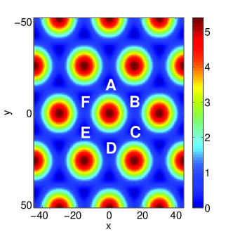
Figure 1: (Color online) A spatial (x-y) contour plot of the ordinary polarization standing wave [lattice beam in Eq. (3)]. In this context, the light intensity maxima correspond to the minima of the resulting refractive index lattice (i.e., honeycomb lattice), as opposed to the focusing nonlinearity lattice field, where they correspond to the maxima (i.e., triangular lattice). Points $A,\,B,\,C,\,D,\,E,\,$ and $F$ are used for naming the various configurations. $A$ is a “nearest-neighbor” minimum of $B$ and $F$, a “next-nearest-neighbor” of $C$ and $E$, and an “opposite” of $D$ (with respect to the local maximum of the lattice). Because of the symmetry of the setup, this is a complete characterization of dipole configurations. We will refer to the configurations with the names given above.

Assuming a stationary state $u(x,y)$ exists, and letting the propagation constant $\mu$ represent the (nonlinear) real eigenvalue of the operator of the right-hand-side of Eq. (1), then the corresponding eigenvector $u(x,y)$ is a fixed point of

$$[\mu-L-N(\textbf{x},|u|^{2})]u=0.$$ (4)

The localized states $u$ of (4) were obtained using the Newton-GMRES fixed point solver nsoli from kell03 and a pseudo arc-length continuation doedel was used to follow each branch and locate the bifurcations which occur at the edge of the first band. Since the parameter of interest is $\mu$, diagnostics are plotted against $\mu$.

We restrict $\mu$ to those values within the first spectral gap of the linear eigenvalue problem,

$$[\mu-L-N(\textbf{x},0)]u=0.$$ (5)

Values of the propagation constant $\mu$ within this forbidden gap in the spectrum of the linearized problem will correspond to exponentially localized in space, so-called gap-soliton, states of the original nonlinear partial differential equation. Using a standard eigenvalue solver package implemented through MATLAB, we identify the spectral gap for our given parameters and gridsize to be $3.62\lesssim\mu\lesssim 4.94$.

The square root of the optical power (or, mathematically, the $L^{2}$ norm) of the localized waves is defined as follows:

$$P=\left[\int_{-\infty}^{\infty}\int_{-\infty}^{\infty}|U|^{2}\,dx\,dy\right]^{1/2}.$$ (6)

Introducing a linearization around an exact stationary solution $u$, and expanding the leading order perturbation into a eigenfunctions and eigenvalues, we obtain the following Bogoliubov system

$$\left[i\lambda+\mu-L-\frac{\partial(NU)}{\partial U}|_{u}\right]\tilde{u}-\frac{\partial(NU)}{\partial U^{*}}|_{u}\tilde{u}^{*}=0,$$

$$\left[i\lambda-\mu+L+\frac{\partial(NU)^{*}}{\partial U^{*}}|_{u}\right]\tilde{u}^{*}+\frac{\partial(NU)^{*}}{\partial U}|_{u}\tilde{u}=0.$$ (7)

We solve the above linear eigenvalue problem using MATLAB’s standard eigenvalue solver package. The symplectic nature of the resulting eigenvalue equations guarantees that the relevant eigenvalues should come in quartets, hence an instability is present whenever the solution of the above linearization problem of Eqs. (7) possesses an eigenvalue with a non-zero real part.

We now briefly discuss the principal stability conclusions, for the defocusing case of ourpre , which we should expect to still be valid in the present configuration. Nearest neighbor excitations in the defocusing case correspond to nearest neighbor excitations in the focusing case, but with an additional $\pi$ phase in the relative phase of the sites added by the so-called staggering transformation ourpre . Therefore, the in-phase nearest neighbor configuration in the defocusing case corresponds to an out-of-phase such configuration in the focusing case (and should thus be stable) pgk_dnls . On the other hand, next nearest neighbor out-of-phase defocusing configurations would correspond to next nearest neighbor out-of-phase focusing configurations and should also be stable (at least in some parameter regimes). By the same token, out-of-phase nearest neighbor, and in-phase next nearest neighbor structures should be unstable. These considerations also indicate that in-phase opposite dipoles should be stable, while out-of-phase such dipoles should always be unstable. Finally, vortex-like structures and in-phase hexapoles should be stable as well. Notice, however, that as discussed in ourpre the multipole structures characterized as potentially stable above will, in fact, typically possess imaginary eigenvalues of negative Krein signature (see e.g. kks and references therein). These may lead to oscillatory instabilities through complex quartets of eigenvalues. These arise by means of Hamiltonian-Hopf bifurcations vdm emerging from collisions with eigenvalues of opposite (i.e., positive) Krein signature. These conclusions will be discussed in connections with our detailed numerical results in what follows.

III Nearest Neighbor Dipole Solitons

In this section, we report dipole solitons where the two lobes of the wave are located in two nearest neighbor (N) lattice sites in the 2D triangular potential shown in Fig. 1. The lobes can have the same phase or $\pi$ phase difference so we define them as in-phase (IP) dipoles and out-of-phase (OP) dipoles, respectively.

III.1 In-Phase Nearest Neighbor Dipole Solitons

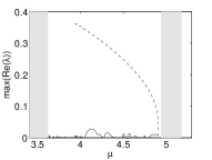
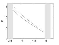
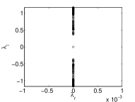
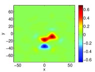
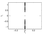
Figure 2: (Color online) The top left panel shows the stability of the dipoles against the propagation constant $\mu$. It is stable when the spectra is purely imaginary (i.e., when $\max({\rm Re}(\lambda))=0$). The top right panel depicts the power of the dipoles against the propagation constant. In each of these images the solution branch is denoted by a solid line. The branch with which the dipole collides and terminates in a saddle-node bifurcation is shown by a dashed line. The shaded areas in both of these panels represent the bands of linear spectrum (5). The middle left and right panels show the profile $u$ of the dipole at $\mu=4$ and the corresponding complex spectral plane $({\rm Re}(\lambda),{\rm Im}(\lambda))$ of $\lambda={\rm Re}(\lambda)+i{\rm Im}(\lambda)$. Finally, the bottom panels show the same features for the unstable saddle solution corresponding to the dashed line.

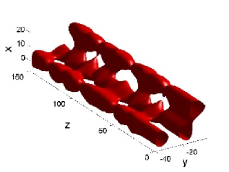
Figure 3: The typical time-dependent dynamics of an unstable configuration along the upper (dashed line) branch of the existence curve presented in the top panels of Fig 2. Depicted here is the isosurface of height $0.15$ of the dynamics of the of the intensity, $|U|^{2}$, of the configuration shown in the bottom panel of Fig. 2.

We have found IP dipoles in adjacent wells for values of the propagation constant $\mu$ throughout the entire Bragg reflection gap for a given $E_{0}$. We found that the solitons exist for $\mu$ between 3.62 and 4.94, and that the intensity of the dipoles cannot be arbitrary low, a result similar to the observed results of the focusing and defocusing cases for square lattices yang04 ; yang04_4 ; our_sq . The relevant findings are summarized in Fig. 2.

The top left panel of Fig. 2 shows the stability of the dipoles against the propagation constant $\mu$, by illustrating the maximal growth rate (maximum real part of all eigenvalues $\lambda$) of perturbations. When $\max({\rm Re}(\lambda))=0$, this implies stability of the configuration, while the configuration is unstable if $\max({\rm Re}(\lambda))\neq 0$ in this Hamiltonian system. We found that this type of dipoles may be stable for windows throughout the first Bragg gap, as predicted above, although it is possible for small oscillatory Hopf instabilities to arise due to opposite signature eigenvalue collisions. The dipole configuration disappears in a saddle-node bifurcation at the edge of the first spectral band, depicted in the top panels of Fig. 2, as $\mu\rightarrow 4.94$, and a real pair of eigenvalues emerges. At this point, the configuration collides with a configuration shown at the bottom panel of Fig. 2 in which the adjacent well next to one of the populated ones becomes excited out-of-phase with the others. Consistent with our theoretical expectation from its having an out-of-phase set of nearest neighbors, the latter configuration always has a real pair of eigenvalues $\lambda$.

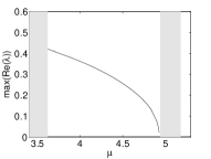
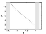
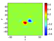
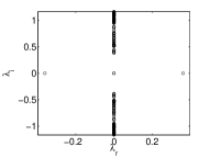
Figure 4: (Color online) The top panels correspond to the same panels of Fig. 2 but for OPN dipole solitons. The bottom panels show the profile $u$ and the corresponding spectral plane of the dipoles at $\mu=4$.

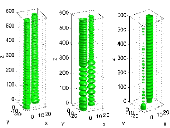
Figure 5: The typical dynamical evolution of an unstable out-of-phase nearest neighbor configuration from the family presented in Fig 4. Depicted is the isosurface at half the maximum of the intial intensity amplitude. Notice that the OPN appears to oscillate between two sites and one for the propagation constant $\mu=4$ (center) of the solution presented in the bottom panels of Fig. 4, as does it for smaller values ($\mu=3.6$, left), although for a larger value of $\mu=4.6$, right, the solution essentially transforms (due to the instability) into a single site mode. We hypothesize that the stronger effect of the nonlinearity on those solutions with smaller values of $\mu$ decreases the size of linear regime, causing these more linearly unstable solutions to actually appear more stable in the full nonlinear dynamical evolution, although it is away from the linear regime that the instability is manifested merely as oscillations.

The middle left and right panels show the profile $u$ of the in-phase nearest (IPN) neighbor dipole at $\mu=4$ and the corresponding spectrum of linearization eigenvalues $\lambda=\lambda_{r}+i\lambda_{i}$ in the complex plane $(\lambda_{r},\lambda_{i})$, respectively. The corresponding profile and spectral plane for the saddle branch (that eventually collides with the IPN solution) at $\mu=4$ is shown in the bottom left and right panel, respectively, of the same figure, illustrating the exponential instability of the latter.

We have simulated the dynamics of the solitary waves when they are unstable. The dipoles are perturbed by a random noise with maximum intensity $2\times 10^{-3}$. It is interesting to note that an unstable IPN dipole turns out to be quite robust, even though it experiences only an oscillatory instability. It is remarkable that up to $z=200$ we did not see any signifant change in the configuration. Therefore, we do not depict our evolution simulation here; we simply note that this is consonant with the very weak growth rate of the relevant oscillatory instability.

For the solution branch shown in the bottom panel of Fig. 2, we present its dynamics in Fig. 3. We found that the instability is strong as predicted above such that even after a relatively short propagation distance, the instability already sets in and leads to recurrent oscillations (for the remainder of our dynamical evolution horizon) between a dipole, two-site state and a three-excited-site state; see Fig. 3.

III.2 Out of Phase Nearest Neighbor Dipole Solitons

We have also found OP dipoles arranged in nearest-neighboring lattice wells which we refer to as OPN. We summarize our findings in Fig. 4 where one can see that the solitons exist in the whole entire region of propagation constant $\mu$ in the first Bragg gap, $\mu\in(3.62,4.94)$. This smooth transition indicates that the OPN dipole solitons emerge out of the Bloch band waves; see e.g. peli04 and shi07 for a relevant discussion of the 1D and of the 2D problem respectively, in the case of the cubic nonlinearity. The OPN dipoles are unstable due to a real eigenvalue pair, as expected from our above theoretical predictions.

As the branch merges with the band edge, we observe an interesting feature, namely that the configuration begins to resemble a hexapole with a $\pi$ phase difference between each well. This can be an indication that these structures bifurcate out of the Bloch band from the same bifurcation point. We elaborate this further in our discussion at the end of section VI.

In Fig. 5 we present the unstable dynamics of OPN dipole solitons perturbed by similar random noise perturbation as in Fig. 3. We display here three solutions for a range of chemical potentials to illustrate that the dynamical evolution of linearly unstable states is apparently correlated to the power of the solution. This type of dipoles is typically more unstable than its IP counterpart, as is illustrated in the figure. In particular, in all three examples of unstable evolution given the instability already starts to manifest itself. around $z=20$ However, for small values of $\mu$ (large power) the OPN continues oscillating between a single site structure and a two site structure for the (longer) evolution distances investigated in this illustrative case, while for large enough $\mu$ (small enough power), one of the sites decays and the power is concentrated on a single site.

IV Next Nearest Neighbor Dipole Solitons

We have also obtained dipole solutions that are not oriented along the two nearest-neighboring lattice wells, but rather where the two humps of the structure are located at two next-nearest-neighboring lattice sites. These humps can once again have the same phase or a $\pi$ phase difference between them. We will again use the corresponding IP and OP designations for these next nearest neighbor waveforms.

IV.1 In Phase, Next Nearest Neighbor Dipole Solitons

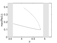
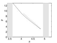
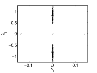
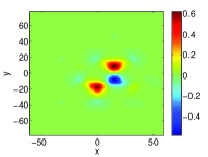
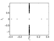
Figure 6: (Color online) The top panels correspond to the same diagnostics as in Fig. 2 but for IPNN dipole solitons. The middle panels show the profile $U$ and the corresponding spectral plane of the IPNN dipole at $\mu=4.1$, while the bottom row shows the same images for the solution branch corresponding to the dashed line in the top panel, shown at the same value of $\mu$.

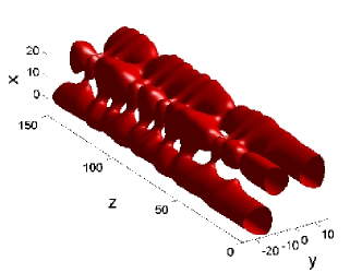
Figure 7: The same figure as Fig. 3, but for the solution presented in the bottom panel of Fig. 6. Depicted is the isosurface of height $0.05$.

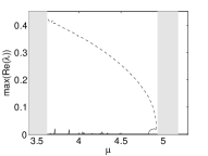
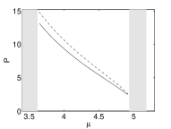
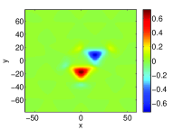
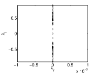
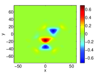
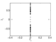
Figure 8: (Color online) The top panels depict the largest real part of the critical eigenvalue, as well as the power of the OPNN dipole solitons. The middle panels show the profile $u$ and the corresponding spectra in the complex plane of the dipole at $\mu=3.9$, and the bottom is the unstable saddle configuration at the same value of $\mu$, where one of the sites has merged with a neighbor out of phase and become an OPN, accounting for the real eigenvalues.

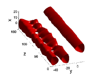
Figure 9: The same figure as Fig. 3, but for the solution presented in the bottom panel of Fig. 8. Depicted is the isosurface of height $0.05$.

The in-phase next-nearest (IPNN) neighbor solitons exist only up to a marginal distance from the second band. The stability and power of these dipoles are shown in Fig. 6. The stability is again consistent with the theoretical discussion of Section II. In particular, the IPNN configuration always possesses a real eigenvalue pair; furthermore, the corresponding unstable “saddle” structure with which it collides and terminates through a saddle-node bifurcation has an additional such eigenvalue pair (two real eigenvalue pairs in total for the solution branch indicated by dashed line in Fig. 6).

We have simulated also the dynamics of the unstable IPNN. Yet, we do not present our simulation here as the typical evolution of this configuration is quite in resemblance to the dynamics of an unstable OPN (see Fig. 5) in the fact that the configuration recurrently oscillates between a two-soliton state and a one-soliton state. Such an oscillation persists even up to $z=200$.

In Fig. 7, we present the dynamical evolution of the bifurcating solution shown in the bottom panel of Fig. 6 under similar random noise perturbation as above. One can note similarities in the typical evolution of this configuration and the evolution of the bifurcating IPN solution shown in Fig. 3, one of which is the recurrent oscillation between a pattern with three pulses and one with just two peaks.

IV.2 Out of Phase Next Nearest Neighbor Dipole Solitons

We have also obtained out-of-phase, next-nearest (OPNN) neighbor dipole solitons. A typical profile of this family of solutions for $\mu=3.9$ is shown in Fig. 8. The power diagram of these solitons is presented in the top panel of Fig. 8. Typically these structures are stable (as indicated again by the comparison with the theoretical discussion and by the numerical results shown in the middle right panel of Fig. 8 ), suffering only windows of oscillatory instability due to the presence of a single eigenvalue with negative signature and its collision with the spectral bands In fact, we have found that a consistent stability range for $E_{0}=8$ exists between $4.5\lesssim\mu\lesssim 4.85$.

For this solution we also observe that, similarly to the IPNN dipoles, the solution disappears at non-zero intensity because of the collision of this dipole with another (three-site) configuration shown in the bottom panels of Fig. 8 in a saddle-node bifurcation. It is relevant to note that the point of the bifurcation is very close to the edge of the Bloch band, i.e., to $\mu\approx 4.94$.

The dynamics of the OPNN dipole do not manifest their very weak oscillatory instability for the evolution distances considered herein. On the other hand, the dynamics of the instability of the three-site solution (with which the OPNN branch collides in the saddle-node bifurcation) can be seen in Fig. 9. More specifically, the instability manifests itself in the form of interactions between the closest out-of-phase pair of solitons (leading to recurrent oscillations between a three-peak and a two-peak state). Notice that the third peak is almost not affected by these interactions.

V Opposite Dipole Solitons

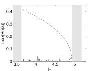
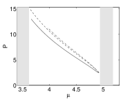
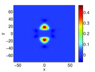
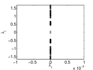
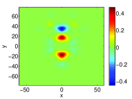
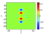
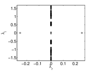
Figure 10: (Color online) The top panels depict the largest real part of the critical eigenvalue, as well as the power and the peak intensity of the IPO dipole solitons. The panels in the second row show the profile $u$ and the corresponding spectra in the complex plane of the dipole at $\mu=4.5$, the third row shows the same images at the same value of $\mu$ for the middle branch (dashed line) of the bifurcation diagram and the bottom row is a solution along the top branch (dash-dotted line) at the same value.

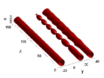
Figure 11: The same figure as Fig. 3, but for the solution presented in the middle panel of Fig. 10. Depicted is the isosurface of height $0.05$.

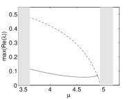
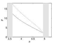
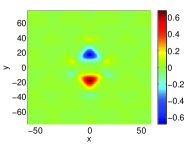
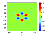
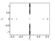
Figure 12: (Color online) The top panels depict the largest real part and the power of the OPO dipole solitons. The middle panels again show the profile $u$ and spectra at $\mu=4$, and the bottom is the more unstable saddle configuration, consisting this time of a hexapole configuration constructed out of three such OPOs.

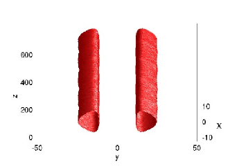
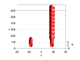
Figure 13: The top panel is the same as Fig. 3, but for the solution presented in the middle panel of Fig. 12, with isosurface of height $0.1$. On the other hand, the bottom panel illustrates again (c.f. Fig.  5) that the linear stability analysis is more predictive of the nonlinear dynamics for the solution with the larger value of $\mu=4.88$ (and accordingly smaller amplitude) close to the intersection with the extended OP quadrupole branch (the isosurface is taken at half the maximum of the initial intensity amplitude). The growth rates for each solution are comparable, while the dynamical evolutions differ drastically.

We now address opposite (O) dipole solitons residing at the two sites along a diameter of a local maximum of the lattice. This is the final type of dipole configuration for a symmetric triangular lattice, exhausting the possibilities up to phase and rotational invariances. Again, we partition our considerations into in-phase and out-of-phase cases.

V.1 In Phase Opposite Dipole Solitons

We have found in-phase opposite (IPO) solitons throughout the first gap in the linear spectrum. Our numerical findings are presented in Fig. 10.

Again, the solution branch is largely stable with small windows of Hopf quartets and again a saddle node bifurcation occurs as the branch approaches the first spectral band. Also, interestingly, the configuration with which this branch collides when it disappears resembles an OPN (or two pairs of OPNs– see the third and fourth row of the figure). The latter branches are naturally unstable due to one (or more) real pair of eigenvalues.

The dynamics of one of the bifurcating solutions, i.e. the configuration with a single OPN structure, is presented in Fig. 11, where one can see that, as usual, only the pair of out-of-phase nearest neighbor dipole interacts, while the other soliton is almost uninfluenced.

Using the same reasoning, one can deduce as well that the dynamics of the other bifurcating solution, presented in the bottom panel of Fig. 10, will be similar, except the fact that now there are two pairs of OPN interacting among themselves.

V.2 Out of Phase Opposite Solitons

Lastly, as regards dipoles, we consider the out of phase opposite (OPO) dipole. The first interesting characteristic of the OPO is its strong instability stemming from a real pair of eigenvalues, seen in the top left and middle rows of Fig.  12. Once again the direct instability of this mode follows from our theoretical considerations of Section II. On the other hand, the figure also reveals an interesting bifurcation structure in this case. The branch actually merges with a hexapole made of three copies of itself close to the band, when solutions start becoming extended. This hexapole then intersects with the linear spectrum shortly thereafter and the solution transforms itself into a fully extended “checkerboard”-like configuration of all adjacent wells excited out-of-phase. As can be seen in the top left and the bottom right of Fig. 12, the hexapole configuration is significantly more unstable, possessing five real eigenvalue pairs.

We have numerically monitored the full evolution to observe the dynamics of the unstable OPO dipoles. It is interesting to note that even though the state has a pair of real eigenvalues, our simulation reveals that the instability is barely detectable for the state depicted in the middle rows of Fig.  12, presumably because of the spatial separation of the populated sites (top row of Figure  13); the solution oscillations are very mild (and almost indetectable) between similar structures with mass concentrated in one site or another. On the other hand, for significantly smaller power (larger $\mu$) as seen in the bottom panel of Figure  13, one site decays fairly rapidly and a robust single site remains.

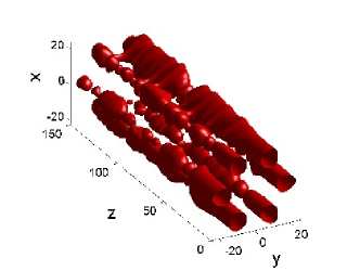
Figure 14: The same dynamical evolution figure as Fig. 3, but for the out-of-phase hexapole depicted in the bottom panel of Fig. 12. Depicted is the isosurface of height $0.1$.

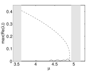
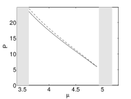
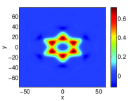
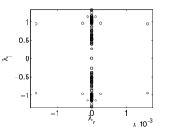
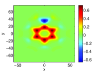
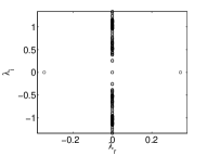
Figure 15: (Color online) The top panels depict the largest real part and the power of the IP hexapole solitons. The middle panels again show the profile $u$ and spectra at $\mu=4$, and the bottom is the more unstable saddle configuration,which features our expected OPN sidekick.

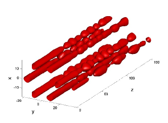
Figure 16: The same figure as Fig. 3, but for the in-phase hexapole depicted in the bottom panel of Fig. 15. Depicted is the isosurface of height $0.3$.

Regarding the bifurcating solution, which is an out-of-phase hexapole, we will explore it as well as the other hexapole configurations in more detail in the following section.

VI Hexapole Solitons and Vortex Necklaces

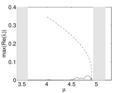
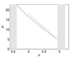
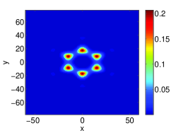
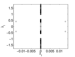
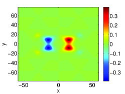
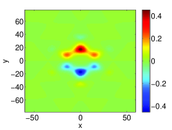
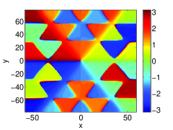
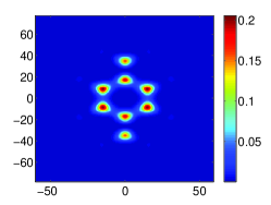
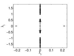
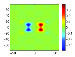
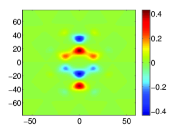
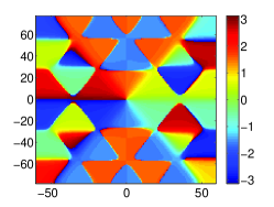
Figure 17: (Color online) The top panels depict the largest real part and the power of the vortex necklace hexapole configuration. The second row depicts the modulus of the solution and corresponding spectrum when $\mu=4.6$. The third row illustrates the real and imaginary components of the field and the phase (from left to right). The fourth and fifth rows show the same properties as the second and third but for the unstable eight-site configuration of the dashed line in the top panels.

Figure 18: The same figure as Fig. 3, but for the vortex necklace with eight lobes depicted in the bottom panel of Fig. 17. Depicted is the isosurface of height $0.1$.

First, we consider the out-of-phase hexapole. The existence and the stability of this configuration has been described in the preceding section. As the state has multiple pairs of real eigenvalues, it is natural to expect that it should be prone to break up under the instability’s dynamical evolution. A typical example of such a numerical experiment is presented in Fig. 14.

We found IP hexapole configurations as well, which, in accordance with our considerations in Section II, turn out to chiefly be stable within the first gap, although they may possess weak oscillatory instability inducing eigenvalue quartets.

This configuration also suffers a saddle-node bifurcation with an OPN-type pair emanating off of one of its lobes, when a neighboring well becomes populated out of phase near the first band. The latter configuration is unstable always possessing a real eigenvalue pair in its linearization spectrum. We note in passing that this is among any of the six equivalent symmetric versions of this configuration.

As for the dynamics of the instability, the solution along the main lower branch is quite robust to strong perturbation. Even though the solution suffers from an oscillatory instability, a random perturbation with a maximum intensity almost $10^{-1}$ cannot lead to a breakup of the configuration until propagation distances of the order of $z=200$. On the other hand, the oscillatory dynamics leading to the break up of the configuration of the bottom panel of Fig. 15 is shown in Fig. 16.

Finally, we investigate the complex-valued hexapole configuration for which each lobe has the same modulus and their phase increases counterclockwise in phase increments of $\pi/6$, yielding a vortex-necklace configuration. This configuration turns out to be stable for the most part within the first gap as well, with minor Hamiltonian Hopf-bifurcation induced oscillatory instabilities. We also found that this solution undergoes a saddle-node bifurcation near the first band, in which it collides with a waveform with two pairs of OPNs. The stability of the latter configuration in the presence of these additional OPN dipoles is consistent with that of their real counterparts from the previous sections, each appearing to contribute one real pair, rendering the relevant configuration quite unstable.

Similar to the case of in-phase hexapoles, even though vortex necklaces may be unstable, they are quite robust to perturbation, given the weak nature of the relevant oscillatory instabilities. We therefore only depict the dynamics of the solutions which have eight lobes as shown in the fourth and fifth row panels of Fig. 17. The typical evolution of this state is shown in Fig. 18, showcasing the oscillatory breakup of this structure into one with a smaller number of lobes.

VII Conclusions

In this communication, we examined in detail theoretically and numerically the existence, stability and dynamics of multipole lattice solitons excited with a saturable defocusing photorefractive nonlinearity in a triangular geometry. We have obtained a wide array of relevant structures, including different types of dipoles and hexapoles, as well as vortices. For the dipole configurations we examined the different possible phase configurations (in phase, and out phase profiles), as well as cases where the excited sites are separated by 0, 1, or 2 intermediate lattices sites. For hexapoles, we examined in phase and out of phase, and we also studied the monotonic increasing phase of a discrete vortex necklace.

We have found good agreement with the general guidelines, explained in section II, stemming from the theoretical analysis of the discrete model. This intuition led to the illustration of a wide variety of potentially stable solutions (although they may incur oscillatory instabilities) such as the in phase, nearest neighbor dipole, the out of phase, next nearest neighbor dipole, and the in phase opposite dipole. We have also identified those solutions including e.g., the out of phase nearest neighbor, in phase next-nearest neighbor, and out of phase opposite dipoles which are typically unstable due to exponential instabilities and real eigenvalues. By the same considerations, the in-phase hexapole was proposed and was indeed found to be typically stable, while the out-of-phase one was predicted and observed to be quite unstable, due to multiple real eigenvalue pairs. Finally, we have seen that the discrete vortex structure is also potentially stable.

Furthermore, we have also identified an interesting set of bifurcations that are associated with the parametric continuation and termination of some of the above branches. The dynamical instabilities encountered in the present work have been monitored through direct integration of the relevant dynamical equation. The result of evolution in every case involved oscillations between the original configuration and one with fewer sites which is more stable, such as a single site solitary wave, and sometimes degeneration to such a configuration. Solutions with smaller power tend to decay into a single site solitary wave for certain solutions investigated, while those with larger power tend to oscillate. This connection is beyond the scope of the present work, but is currently being investigated further.

Since the framework of defocusing equations has been studied far less extensively than their focusing counterparts, it would be particularly interesting to extend the present considerations to other structures. Perhaps the most interesting example would be the study of multiple charge vortices in this context which would be an interesting endeavor both from a theoretical, as well as from an experimental point of view. Such studies are currently in progress and will be reported in future publications.

Acknowledgements. PGK acknowledges support from NSF-DMS-0505663, NSF-DMS-0619492 and NSF-CAREER. W. Krolikowski is gratefully acknowledged for numerous informative discussions on the theme of this work.

References

- (1) N.K. Efremidis, S. Sears, D. N. Christodoulides, J. W. Fleischer, and M. Segev Phys. Rev. E 66, 46602 (2002).
- (2) J.W. Fleischer, M. Segev, N.K. Efremidis and D.N. Christodoulides, Nature 422, 147 (2003); J.W. Fleischer, T. Carmon, M. Segev, N.K. Efremidis and D.N. Christodoulides, Phys. Rev. Lett. 90, 23902 (2003).
- (3) D. Neshev, E. Ostrovskaya, Yu.S. Kivshar and W. Krolikowski, Opt. Lett. 28, 710 (2003).
- (4) H. Martin, E.D. Eugenieva, Z. Chen and D.N. Christodoulides, Phys. Rev. Lett. 92, 123902 (2004).
- (5) J. Yang, I. Makasyuk, A. Bezryadina, and Z. Chen, Opt. Lett. 29, 1662 (2004).
- (6) J. Yang, I. Makasyuk, P. G. Kevrekidis, H. Martin, B. A. Malomed, D. J. Frantzeskakis, and Zhigang Chen, Phys. Rev. Lett. 94, 113902 (2005).
- (7) D. Neshev, Yu. S. Kivshar, H. Martin, and Z. Chen, Opt. Lett. 29, 486-488 (2004).
- (8) X. Wang, Z. Chen, and P. G. Kevrekidis, Phys. Rev. Lett. 96, 083904 (2006).
- (9) D. N. Neshev, T.J. Alexander, E.A. Ostrovskaya, Yu.S. Kivshar, H. Martin, I. Makasyuk and Z. Chen, Phys. Rev. Lett. 92, 123903 (2004); J. W. Fleischer, G. Bartal, O. Cohen, O. Manela, M. Segev, J. Hudock, and D.N. Christodoulides Phys. Rev. Lett. 92, 123904 (2004).
- (10) B. Freedman, G. Bartal, M. Segev, R. Lifshitz, D.N. Christodoulides and J.W. Fleischer, Nature 440, 1166 (2006).
- (11) T. Schwartz, G. Bartal, S. Fishman and M. Segev, Nature 446, 52 (2007).
- (12) D. N. Christodoulides, F. Lederer, and Y. Silberberg, Nature 424, 817 (2003); A. A. Sukhorukov, Y. S. Kivshar, H. S. Eisenberg, and Y. Silberberg, IEEE J. Quant. Elect. 39, 31 (2003).
- (13) S. Aubry, Physica 103D, 201 (1997); S. Flach and C. R. Willis, Phys. Rep. 295, 181 (1998); D. K. Campbell, S. Flach, and Y. S. Kivshar, Phys. Today, January 2004, p. 43.
- (14) V. A. Brazhnyi and V. V. Konotop, Mod. Phys. Lett. B 18, 627 (2004); P. G. Kevrekidis and D. J. Frantzeskakis, Mod. Phys. Lett. B 18, 173 (2004).
- (15) O. Morsch and M. Oberthaler, Rev. Mod. Phys. 78, 179 (2006).
- (16) P.G. Kevrekidis, B.A. Malomed and Yu.B. Gaididei, Phys. Rev. E 66, 016609 (2002).
- (17) M.J. Ablowitz, B. Ilan, E. Schonbrun and R. Piestun, Phys. Rev. E 74, 035601 (2006).
- (18) B. Freedmna, G. Bartal, M. Segev, R. Lifshitz, D.N. Christodoulides and J.W. Fleischer, Nature (London) 440, 1166 (2006).
- (19) C.R. Rosberg, D.N. Neshev, A.A. Sukhorukov, W. Krolikowski and Yu.S. Kivshar, Opt. Lett. 32, 397 (2007).
- (20) T.J. Alexander, A.S. Desyatnikov and Yu.S. Kivshar, Opt. Lett. 32, 1293 (2007).
- (21) O. Peleg, G. Bartal, B. Freedman, O. Manela, M.Segev, and D. Christodoulides, Phys. Rev. Lett. 98, 103901 (2007).
- (22) L. Tang, C. Lou, X. Wang, D. Song, X. Chen, J. Xu, Z. Chen, H. Susanto, K. Law and P.G. Kevrekidis, Opt. Lett. 32, 3011 (2007).
- (23) P.G. Kevrekidis, H. Susanto and Z. Chen, Phys. Rev. E 74, 066606 (2006).
- (24) P.G. Kevrekidis, K.Ø. Rasmussen and A.R. Bishop, Int. J. Mod. Phys. B 15, 2833 (2001); D.E. Pelinovsky, P.G. Kevrekidis and D.J. Frantzeskakis, Physica D 212, 1 (2005); ibid 212, 20 (2005).
- (25) J. Yang, New J. Phys. 6, 47 (2004).
- (26) J. Yang, A. Bezryadina, I. Makasyuk and Z. Chen, Stud. Appl. Math. 113, 389 (2004).
- (27) H. Susanto, K. Law, P.G. Kevrekidis, L. Tang, C. Lou, X. Wang and Z. Chen, Dipole and quadrupole solitons in two-dimensional defocusing photonic lattices. preprint (2007).
- (28) C. T. Kelley, Solving Nonlinear Equations with Newton s Method, no. 1 in Fundamentals of Algorithms, SIAM, Philadelphia, 2003.
- (29) E. Doedel. International Journal of Bifurcation and Chaos. 7(9):2127-2143, 1997.
- (30) T. Kapitula, P.G. Kevrekidis, B. Sandstede, Physica D 195 263 (2004).
- (31) J.-C. van der Meer, Nonlinearity 3, 1041 (1990).
- (32) D. Pelinovsky, A.A. Sukhorukov, and Yu.S. Kivshar, Phys. Rev. E 70, 036618 (2004).
- (33) Z. Shi and J. Yang, Phys. Rev. E 75, 056602 (2007).