Critical properties of a dilute O($n$) model on the kagome lattice

Abstract

A critical dilute O($n$) model on the kagome lattice is investigated analytically and numerically. We employ a number of exact equivalences which, in a few steps, link the critical O($n$) spin model on the kagome lattice to the exactly solvable critical $q$-state Potts model on the honeycomb lattice with $q=(n+1)^{2}$. The intermediate steps involve the random-cluster model on the honeycomb lattice, and a fully packed loop model with loop weight $n^{\prime}=\sqrt{q}$ and a dilute loop model with loop weight $n$, both on the kagome lattice. This mapping enables the determination of a branch of critical points of the dilute O($n$) model, as well as some of its critical properties. For $n=0$, this model reproduces the known universal properties of the $\theta$ point describing the collapse of a polymer. For $n\neq 0$ it displays a line of multicritical points, with the same universal properties as a branch of critical behavior that was found earlier in a dilute O($n$) model on the square lattice. These findings are supported by a finite-size-scaling analysis in combination with transfer-matrix calculations.

I Introduction

The first exact results N for the O($n$) critical properties were obtained for a model on the honeycomb lattice, and revealed not only the critical point, but also some universal parameters of the critical state, as well as the low-temperature phase, as a function of $n$. The derivation of these results depends on a special choice of the O($n$)-symmetric interaction between the $n$-component spins of the O($n$) model, which enables a mapping on a loop gas DMNS . These results were supposed to apply to a whole universality class of O($n$)-symmetric models in two dimensions.

Since then, also O($n$) models on the square and triangular lattices were investigated BN ; KBN . Indeed, branches were found with the same universal properties as the honeycomb model, but in addition to these, several other branches of critical behavior were reported. Among these, we focus on ‘branch 0’ as reported in Refs. BN ; KBN . The points on this branch appear to describe a higher critical point. For $n=0$, it can be identified with the so-called $\theta$ point DS describing the collapse of a polymer in two dimensions, which has been interpreted as a tricritical O($n=0$) model. It has indeed been found that the introduction of a sufficiently strong and suitably chosen attractive potential between the loop segments changes the ordinary O($n=0$) transition into a first-order one BBN , such that this change precisely coincides with the $n=0$ point of branch 0. Thus, the $\theta$ point plays the role of a tricritical O($n=0$) transition. Furthermore, it has been verified that tricriticality in the O($n$) model can be introduced by adding a sufficient concentration of vacancies into the system GNB . More precisely, the introduction of vacancies leads to a branch of higher critical points, of which the points $n=0$ and $n=1$ belong to universality classes (of the $\theta$ point and the tricritical Blume-Capel model respectively) that have been described earlier as tricritical points.

However, the critical points of branch 0 on the square lattice appear to display universal properties that are different from those of the branch of higher critical points of the O($n$) model with vacancies GNB , except at the intersection point of the two branches at $n=0$. It thus appears that the continuation of the $\theta$ point at $n=0$ to $n\neq 0$ can be done in different ways, leading to different universality classes. In order to gain further insight in this situation, the present work considers an O($n$) loop model on the kagome lattice with the purpose to find a $\theta$-like point, to continue this point to $n\neq 0$ and to explore the resulting universality.

II Mappings

The partition function of the spin representation of $q$-state Potts model on the honeycomb lattice

$$Z_{\rm Potts}=\sum_{\{S\}}\exp\left(K\sum_{<i,j>}\delta_{s_{i},s_{j}}\right)$$ (1)

depends on the temperature $T$ by the coupling $K=J/k_{\rm B}T$, where $J$ is the nearest-neighbor spin-spin interaction. The spins $s_{i}$ can assume values 1, 2, $\cdots$, $q$ and their index $i$ labels the sites of the honeycomb lattice. The first summation is over all possible spin configurations $\{S\}$, and the second one is over the nearest neighbor spin pairs. This Potts model can be subjected to a series of mappings which lead, via the random-cluster model and a fully-packed loop model, to a dilute O($n$) loop model which can also be interpreted as an O($n$) spin model.

II.1 Honeycomb Potts model to fully-packed kagome loop model

The introduction of bond variables, and a summation on the spin variables map the Potts model onto the random-cluster (RC) model KF , with partition function

$$Z_{\rm RC}(u,q)=\sum_{\mathcal{B}}u^{N_{b}}q^{N_{c}}\,,$$ (2)

where $N_{b}$ is the number of bonds, $N_{c}$ the number of clusters, and $u\equiv e^{K}-1$ the weight of a bond. The sum is on all configurations ${\mathcal{B}}$ of bond variables: each bond variable is either 1 (present) or 0 (absent). In Eq. (2), $q$ can be considered a continuous real number, playing the role of the weight of a cluster. Here, a cluster is either a single site or a group of sites connected together by bonds on the lattice. A typical configuration of the RC model on the honeycomb lattice is shown in Fig. 1.

The next step is a mapping of the RC model on the honeycomb lattice onto a fully packed loop (FPL) model on the kagome lattice, which proceeds similarly as in the case of the square lattice BKW . The sites of FPL model sit in the middle of the edges of the honeycomb lattice, and thus form a kagome lattice IS . Fully packed here means that all edges of the kagome lattice are covered by loop segments. The one-to-one correspondence between these two configurations is established by requiring that the loops do not intersect the occupied edges (bonds) of the honeycomb RC model, and always intersect the empty edges, as illustrated in Fig. 1.

Figure 1: Mapping of the RC model onto a FPL model. The sites of the honeycomb lattice are shown as black circles. The dashed and the thin solid lines display the empty and the occupied edges (bonds) of the RC model on the honeycomb lattice respectively. The RC configuration is here represented by an FPL configuration on the surrounding lattice, i.e., the kagome lattice. Its loops (bold solid lines) follow the boundaries of the random clusters, both externally and internally. The Boltzmann weight of this finite-size configuration of the RC configuration is $u^{12}q^{19}$ according to Eq. (2), and that of the corresponding FPL configuration is $a_{1}^{12}a_{2}^{26}n^{20}$ according to Eq. (3).

To specify the Boltzmann weights of the FPL model, we assign a weight $n$ to each loop, a weight $a_{1}$ to each vertex where the loop segments do not intersect an edge which is occupied by a bond of the RC model, and a weight $a_{2}$ to each vertex where the loop segments intersect an edge which is empty in the RC model, as illustrated in Fig. 2.

Figure 2: Vertex weights of the FPL model. The bold solid lines represent loop segments. The weight of vertex where the loops do not intersect a bond (thin solid line) is $a_{1}$. The weight of a vertex where two loops intersect an unoccupied edge (dashed line) is $a_{2}$.

The partition function of the FPL model on the kagome lattice is thus defined as

$$Z_{\rm FPL}^{\rm kag}(a_{1},a_{2},n)=\sum_{\mathcal{F}}a_{1}^{m_{1}}a_{2}^{m_{2}}n^{m_{l}}\,,$$ (3)

where $m_{1}$ is the number of type-1 vertices, $m_{2}$ is the number of type-2 vertices and $m_{l}$ the number of loops. The sum is on all configurations $\mathcal{F}$ of loops covering all the edges of the kagome lattice.

The one-to-one correspondence between RC configurations and FPL configurations makes it possible to express the configuration parameters $m_{1}$, $m_{2}$ and $m_{l}$ of the FPL in those of the RC model, namely $N_{b}$ and $N_{c}$. Each vertex of type-1 corresponds with a bond of the RC model on the honeycomb lattice, thus

$$m_{1}=N_{b}\,.$$ (4)

The total number of the two kinds of vertices is equal to the number of edges on the honeycomb lattice, i.e.,

$$m_{1}+m_{2}=\frac{3N}{2}\,,$$ (5)

where $N$ is the total number of sites of the honeycomb lattice. Here we ignore surface effects of finite lattices. Furthermore, a loop on the kagome lattice is either one surrounding a random cluster on the honeycomb lattice, or one following the inside of a loop formed by the bonds of a random cluster. Thus

$$m_{l}=N_{c}+N_{l}\,,$$ (6)

where $N_{l}$ is the loop number of the RC model. Together with the Euler relation

$$N_{c}=N-N_{b}+N_{l}\,,$$ (7)

Eqs. (4) to (6) yield the numbers of vertices and loops on the kagome lattice as

$$m_{1} = N_{b}$$

$$m_{2} = 3N/2-N_{b}$$ (8)

$$m_{l} = 2N_{c}+N_{b}-N\,.$$

Substitution in the partition function (3) leads to

$$Z_{\rm FPL}^{\rm kag}=\left(\frac{a_{2}^{\frac{3}{2}}}{n}\right)^{N}\sum_{\mathcal{F}}\left(\frac{a_{1}n}{a_{2}}\right)^{N_{b}}(n^{2})^{N_{c}}\,.$$ (9)

The weight of a given loop configuration is thus equal to the corresponding RC weight $u^{N_{b}}q^{N_{c}}$ if

$$n = \sqrt{q}$$

$$a_{1} = uq^{-\frac{1}{6}}$$ (10)

$$a_{2} = q^{\frac{1}{3}}\,,$$

which completes the mapping of the RC onto the FPL model.

II.2 Fully-packed loop model to dilute loop model

Next we map the FPL model on the kagome lattice onto a dilute loop (DL) model on the same lattice, using a method due to Nienhuis (see e.g. Ref. BN ). The partition function of the FPL model on the kagome lattice is slightly rewritten as

$$Z_{\rm FPL}^{\rm kag}=(a_{1}+a_{2})^{\frac{3N}{2}}\sum_{{\mathcal{F}}}w_{1}^{m_{1}}w_{2}^{m_{2}}[(n-1)+1]^{m_{l}}$$ (11)

with $w_{1}=a_{1}\big{/}(a_{1}+a_{2})$ and $w_{2}=a_{2}\big{/}(a_{1}+a_{2})$. Eq. (11) invites an interpretation in terms of colored loops, say red with loops of weight $n-1$ and green loops of weight 1. Each of the $2^{m_{l}}$ terms in the expansion of $[(n-1)+1]^{m_{l}}$ thus specifies a way to color the loops:

$$[(n-1)+1]^{m_{l}}=\sum_{\{\rm colorings\}}(n-1)^{l_{r}}1^{l_{g}}\,,$$

where $l_{r}$ and $l_{g}$ denote the number of red loops and green loops respectively, $l_{r}+l_{g}=m_{l}$. Let $\mathcal{C}$ denote a graph $\mathcal{F}$ in which the colors of all loops are specified. The partition sum can thus be expressed in terms of a summation over all colored loop configurations $\mathcal{C}$. The vertices of the kagome lattice are visited by two colored loops, and can thus be divided into 6 types, shown in Fig. 3 with their associated weights $x_{1}=y_{1}=z_{1}=w_{1}$ and $x_{2}=y_{2}=z_{2}=w_{2}$.

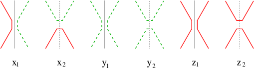
Figure 3: (color online). Weights of colored vertices. The vertical solid lines represent occupied edges (bonds) on the honeycomb lattice, while broken lines stand for empty edges. The bold solid lines represent the red loop segments, and the bold dashed lines the green ones.

Thus, Eq. (11) assumes the form

$$Z^{\rm kag}_{\rm FPL}=(a_{1}+a_{2})^{\frac{3N}{2}}\sum_{\mathcal{C}}x_{1}^{N_{x_{1}}}x_{2}^{N_{x_{2}}}y_{1}^{N_{y_{1}}}y_{2}^{N_{y_{2}}}z_{1}^{N_{z_{1}}}z_{2}^{N_{z_{2}}}(n-1)^{l_{r}}1^{l_{g}}\,.$$ (12)

The sum $\sum_{\mathcal{C}}$ on all colored loop configurations may now be replaced by two nested sums, the first of which is a sum $\sum_{\mathcal{R}}$ on all dilute loop configurations of red loops, and the second sum $\sum_{\mathcal{G}|\mathcal{R}}$ is on all configurations of green loops $\mathcal{G}$ that are consistent with $\mathcal{R}$, i.e., the green loop configurations that cover all the kagome edges not covered by a red loop. Thus

$$Z^{\rm kag}_{\rm FPL}=(a_{1}+a_{2})^{\frac{3N}{2}}\sum_{\mathcal{R}}x_{1}^{N_{x_{1}}}x_{2}^{N_{x_{2}}}z_{1}^{N_{z_{1}}}z_{2}^{N_{z_{2}}}(n-1)^{l_{r}}\sum_{\mathcal{G}|\mathcal{R}}y_{1}^{N_{y_{1}}}y_{2}^{N_{y_{2}}}1^{l_{g}}\,.$$ (13)

For each vertex visited by green loops only, there are precisely two possible local loop configurations. Since the loop weight of the green loops is 1, the summation over such pairs of configurations is trivial:

$$\sum_{\mathcal{G}|\mathcal{R}}y_{1}^{N_{y_{1}}}y_{2}^{N_{y_{2}}}1^{l_{g}}=\sum_{\mathcal{G}|\mathcal{R}}y_{1}^{N_{y_{1}}}y_{2}^{N_{y_{2}}}=(y_{1}+y_{2})^{N_{g}}=1\,,$$ (14)

where $N_{g}$ is the number of green-only vertices. The FPL partition sum thus reduces to that of a dilute loop model, involving only red loops of weight $n-1$:

$$Z^{\rm kag}_{\rm FPL}(a_{1},a_{2},n)=(a_{1}+a_{2})^{\frac{3N}{2}}Z_{\rm DL}^{\rm kag}(x_{1},x_{2},z_{1},z_{2},n-1)\,,$$ (15)

where the partition function of the dilute loop model is defined as

$$Z_{\rm DL}^{\rm kag}(x_{1},x_{2},z_{1},z_{2},n)\equiv\sum_{{\mathcal{L}}}x_{1}^{N_{x_{1}}}x_{2}^{N_{x_{2}}}z_{1}^{N_{z_{1}}}z_{2}^{N_{z_{2}}}n^{N_{l}}\,,$$ (16)

in which we forget the color variable, and denote the number of loops in a dilute configuration $\mathcal{L}$ as $N_{l}$. The dilute vertices are shown in Fig. 4, together with their weights. The exponents of the vertex weights in Eq. (16) represent the numbers of the corresponding vertices. Because of the similarity with the derivation of branch 0 on the square lattice, we refer to the model (16) as branch 0 of the kagome O($n$) loop model.

The transformation between the FPL and the DL model is illustrated in Fig. 5.

Figure 4: The five vertex weights for the dilute loop model. The vertex with weight 1 results from a summation involving the weights of vertices 3 and 4 in Fig. 3.

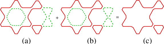
Figure 5: (color online). Partial summation on the green loops. The solid lines represent red loops, and the dashed lines green loops. For a fixed configuration of red loops, each vertex visited only by green loops has two possible weights: $y_{1}$ or $y_{2}$ (see Fig. 3). For the simple case shown here, there are two possible configurations (a) and (b), of which the relative weights are $x_{1}^{6}x_{2}^{2}y_{1}z_{1}z_{2}(n-1)^{2}1^{2}$ and $x_{1}^{6}x_{2}^{2}y_{2}z_{1}z_{2}(n-1)^{2}1^{3}$ respectively. Addition of these weights yields the weight $x_{1}^{6}x_{2}^{2}z_{1}z_{2}(n-1)^{2}$ of the DL configuration shown in (c).

II.3 Dilute loop model to O($n$) spin model

The Boltzmann weights in Eq. (16) contain, besides the loop weights, only local weights associated with the vertices of the kagome lattice. Just as in the case of the O($n$) model on the square lattice described in Ref. BN , there are precisely four incoming edges at each vertex. This implies that there is an equivalent O($n$) spin model:

$$Z_{\rm DL}^{\rm kag}(x_{1},x_{2},z_{1},z_{2},n)=Z_{\rm spin}(x_{1},x_{2},z_{1},z_{2})\,,$$ (17)

of which the local weights have the same relation with the vertex weights as for the square lattice model of Ref. BN . Thus, the partition sum of the spin model is expressed by

$$Z_{\rm spin}(x_{1},x_{2},z_{1},z_{2})\equiv\int\left[\prod_{i}d\vec{s}_{i}\right]\prod_{v}[1+x_{1}(\vec{s}_{v1}\cdot\vec{s}_{v2}+\vec{s}_{v3}\cdot\vec{s}_{v4})+\mbox{\hskip 28.45274pt}$$

$$\mbox{\hskip 56.9055pt}x_{2}(\vec{s}_{v1}\cdot\vec{s}_{v4}+\vec{s}_{v2}\cdot\vec{s}_{v3})+z_{1}(\vec{s}_{v1}\cdot\vec{s}_{v2})(\vec{s}_{v3}\cdot\vec{s}_{v4})+z_{2}(\vec{s}_{v1}\cdot\vec{s}_{v4})(\vec{s}_{v2}\cdot\vec{s}_{v3})]\,.$$ (18)

The product is on all vertices $v$ of the kagome lattice. The spins $\vec{s}_{vi}$ sit on the midpoints of the edges of the kagome lattice. Their subscript “$vi$” specifies the vertex $v$ as well as the position $i$ (with $1\leq i\leq 4$) with respect to the vertex. The label $1$ runs clockwise around each vertex, such that the spins $\vec{s}_{v1}$ and $\vec{s}_{v2}$ sit on the same side of the honeycomb edge passing through vertex $v$. The spins have $n$ Cartesian components and are normalized to length $\sqrt{n}$. There are two different notations for each spin (because each spin is adjacent to two vertices), but a given subscript $vi$ refers to only one spin. Here the number $n$ is restricted to positive integers, of which only the case $n=1$ is expected to be critical.

II.4 Condition for criticality

Since the critical point of the RC model on the honeycomb lattice is known Wufy as a function of $q$, namely

$$(u_{\rm hc}^{\rm c})^{3}-3q(u_{\rm hc}^{\rm c})+q^{2}=0\,,$$ (19)

the corresponding critical point of the $n=\sqrt{q}$ FPL model on the kagome lattice is also known. According to Eq. (10)

$$a_{1}^{\rm c} = u_{\rm hc}^{\rm c}q^{-\frac{1}{6}}$$

$$a_{2}^{\rm c} = q^{\frac{1}{3}}\,,$$ (20)

from which the corresponding critical point of the DL model with loop weight $n=\sqrt{q}-1$ on the kagome lattice follows as

$$x_{1}^{\rm c} = z_{1}^{\rm c}=\frac{u_{\rm hc}^{\rm c}}{u_{\rm hc}^{\rm c}+\sqrt{q}}$$

$$x_{2}^{\rm c} = z_{2}^{\rm c}=\frac{\sqrt{q}}{u_{\rm hc}^{\rm c}+\sqrt{q}}\,.$$ (21)

III Derivation of some critical properties

The transformations described in Sec. II leave (apart from a shift by a constant) the free energy unchanged, and lead to relations between the thermodynamic observables of the various models. Thus, the conformal anomaly and some of the critical exponents of the FPL and the DL models can be obtained from the existing results for the random-cluster model. Thus, like in the analogous case of the O($n$) model on the square lattice BN , the FPL model on the kagome lattice should be in the universality class of the low-temperature O($n$) phase. However, the representation of magnetic correlations in our present cylindrical geometry leads to a complication. The kagome lattice structure, together with the FPL constraint, imposes the number of loop segments running along the cylinder to be even. Since the O($n$) spin-spin correlation function is represented by a single loop segment in the loop representation, which cannot be embedded in an FPL model on the kagome lattice, it is not clear how to represent magnetic correlations in this model. Thus we abstain from a further discussion of the scaling dimensions of the FPL model.

1. conformal anomaly

For the FPL model with loop weight $n$ on the kagome lattice, the conformal anomaly $c$ is equal to that of the $n=\sqrt{q}$ Potts model BCN ; Affl :

$$c=1-\frac{6}{m(m+1)},~{}~{}~{}~{}2\cos\frac{\pi}{m+1}=n,~{}~{}~{}~{}m\geq 1\,.$$ (22)

In the Coulomb gas language BN2 , it can be expressed as a function of the Coulomb gas coupling constant $g$, with $g=m/(m+1)$:

$$c=1-\frac{6(1-g)^{2}}{g},~{}~{}~{}~{}2\cos(\pi g)=-n,~{}~{}~{}~{}0\leq g\leq 1\,.$$ (23)

The conformal anomaly $c$ of the branch-$0$ critical O($n$) DL model on the kagome lattice with loop weight $n$ is given by the same formula, but with $n$ replaced by $n+1$:

$$c=1-\frac{6}{m(m+1)},~{}~{}~{}~{}2\cos\frac{\pi}{m+1}=n+1,~{}~{}~{}~{}m\geq 1\,.$$ (24)

The conformal anomaly is, via the number $m$, related to a set of scaling dimensions $X_{i}$ as determined by the Kac formula FQS :

$$X_{i}=\frac{[p_{i}(m+1)-q_{i}m]^{2}-1}{2m(m+1)}\,,$$ (25)

where $p_{i}$ and $q_{i}$ are integers for unitary models.

2. temperature exponent

For the branch-$0$ critical DL model with loop weight $n$ on the kagome lattice, the temperature exponent is expected to be the same as that for branch 0 on the square lattice BN , namely $X_{t}=X_{i}$ with $p_{i}=m,q_{i}=m$ in Eq. (25).

3. magnetic exponent

The magnetic exponent of the branch-$0$ DL model with $n=0$ on the kagome lattice is not equal to the magnetic exponent of the low temperature O($n+1$) loop model. The same situation was found earlier for the branch-$0$ O($0$) model on the square lattice BN . According to the reason given in BN , the magnetic exponent is equal to the temperature one, i.e., the $p_{i}=m,q_{i}=m$ entry of Eq. (25). The geometry of the underlying FPL model, where the number of dangling bonds is restricted to be even, plays here an essential role. Note that the magnetic exponent of the tricritical dilute O($n$) model GNB , even at the $\theta$ point, is different from that of branch 0.

These results for $X_{t}$ and $X_{h}$ are expressed in the Coulomb gas language as

$$X_{t}=X_{h}=1-1/2g\,.$$ (26)

IV Numerical verification

IV.1 Construction of the transfer matrix

The transfer matrix is constructed for an $L\times M$ loop model wrapped on a cylinder, with its axis perpendicular to one of the lattice edge directions of the kagome lattice. The finite size $L$ is defined such that the circumference of the cylinder is spanned by $L/2$ elementary hexagons (corner to corner). The cylinder is divided into $M$ slices, of which $L$ sites form a cyclical row, while each of the $L/2$ remaining sites forms an equilateral triangle with two of the sites of the cyclical row. The length of the cylinder is thus $M\sqrt{3}$.

The partition function of this finite-size DL model is given by Eq. (3), but with ${\mathcal{L}}_{M}$ instead of ${\mathcal{L}}$, in order to specify the length $M$ of the cylinder:

$$Z^{(M)}=\sum_{{\mathcal{L}}_{M}}x_{1}^{N_{x_{1}}}x_{2}^{N_{x_{2}}}z_{1}^{N_{z_{1}}}z_{2}^{N_{z_{2}}}n^{N_{l}}\,.$$ (27)

There are open boundaries at both ends of the cylinder, so that there are $L$ dangling edges connected to the vertices on row $1$, as well as on row $M$. The way in which the end points of the dangling edges are pairwise connected by the loop configuration ${\mathcal{L}}_{M}$ is defined as the ‘connectivity’, see Ref. BN for details. Here we ignore the dangling edges of row 1 (except for a topological property that will be considered later) and focus on the $L$ dangling edges of row $M$. Since it is determined by the loop configuration, the connectivity $\beta$ at row $M$ is written as a function of ${\mathcal{L}}_{M}$: $\beta=\varphi({\mathcal{L}}_{M})$. The partition sum is divided into a number of restricted sums $Z_{\beta}^{(M)}$, each of which collects all terms in $Z^{(M)}$ having connectivity $\beta$ on row $M$, i.e.:

$$Z^{(M)}=\sum_{\beta}Z^{(M)}_{\beta}\,,\mbox{\hskip 28.45274pt}Z^{(M)}_{\beta}=\sum_{{\mathcal{L}}_{M}}\delta_{\beta,\varphi({\mathcal{L}}_{M})}x_{1}^{N_{x_{1}}}x_{2}^{N_{x_{2}}}z_{1}^{N_{z_{1}}}z_{2}^{N_{z_{2}}}n^{N_{l}}\,.$$ (28)

An increase of the system length $M$ to $M+1$ leads to a new configuration ${\mathcal{L}}_{M+1}$ which can be decomposed in ${\mathcal{L}}_{M}$ and the appended configuration $l_{M+1}$ on row $M+1$. The graph $l_{M+1}$ fits the dangling edges of the loop graph ${\mathcal{L}}_{M}$ on the $M$-row lattice. The addition of the new row increases the number of the four kinds of vertices and of the number of loops by $n_{x_{1}}$, $n_{x_{2}}$, $n_{z_{1}}$, $n_{z_{2}}$ and $n_{l}$ respectively. The restricted partition sum of the system with $M+1$ rows is

$$Z_{\alpha}^{(M+1)}=\sum_{{\mathcal{L}}_{M+1}}\delta_{\alpha,\varphi({\mathcal{L}}_{M+1})}x_{1}^{N_{x_{1}}+n_{x_{1}}}x_{2}^{N_{x_{2}}+n_{x_{2}}}z_{1}^{N_{z_{1}}+n_{z_{1}}}z_{2}^{N_{z_{2}}+n_{z_{2}}}n^{N_{l}+n_{l}}=$$

$$\sum_{{\mathcal{L}}_{M}}x_{1}^{N_{x_{1}}}x_{2}^{N_{x_{2}}}z_{1}^{N_{z_{1}}}z_{2}^{N_{z_{2}}}n^{N_{l}}\\ \sum_{{l}_{M+1}|{\mathcal{L}}_{M}}\delta_{\alpha,\varphi({\mathcal{L}}_{M+1})}x_{1}^{n_{x_{1}}}x_{2}^{n_{x_{2}}}z_{1}^{n_{z_{1}}}z_{2}^{n_{z_{2}}}n^{n_{l}}\,.$$ (29)

The last sum is on all sub-graphs ${l}_{M+1}$ that fit ${\mathcal{L}}_{M}$. The connectivity $\varphi({\mathcal{L}}_{M+1})$ depends only on the connectivity $\beta$ on row $M$, and on $l_{M+1}$, so that we may write $\varphi({\mathcal{L}}_{M+1})=\psi(\beta,l_{M+1})$. Thus Eq. (29) assumes the form

$$Z_{\alpha}^{(M+1)}=\sum_{\beta}\sum_{{\mathcal{L}}_{M}}\delta_{\beta,\varphi({\mathcal{L}}_{M})}x_{1}^{N_{x_{1}}}x_{2}^{N_{x_{2}}}z_{1}^{N_{z_{1}}}z_{2}^{N_{z_{2}}}n^{N_{l}}\\ \sum_{l_{M+1}|\beta}\delta_{\alpha,\psi(\beta,l_{M+1})}x_{1}^{n_{x_{1}}}x_{2}^{n_{x_{2}}}z_{1}^{n_{z_{1}}}z_{2}^{n_{z_{2}}}n^{n_{l}}\,.$$ (30)

The third sum depends only on $\alpha$ and $\beta$, and thus defines the elements of the transfer matrix $\mathbf{T}$ as

$$T_{\alpha\beta}\equiv\sum_{l_{M+1}|\beta}\delta_{\alpha,\psi(\beta,l_{M+1})}x_{1}^{n_{x_{1}}}x_{2}^{n_{x_{2}}}z_{1}^{n_{z_{1}}}z_{2}^{n_{z_{2}}}n^{n_{l}}\,,$$ (31)

Substitution of $T_{\alpha\beta}$ and Eq. (28) in Eq. (30) then yields the recursion of the restricted partition sum as

$$Z_{\alpha}^{(M+1)}=\sum_{\beta}T_{\alpha\beta}Z_{\beta}^{(M)}\,.$$ (32)

In order to save memory and computer time, the transfer matrix of a system with finite size $L$ is decomposed in $\frac{3L}{2}$ sparse matrices:

$$T=T_{\frac{L}{2}+L}\cdot T_{\frac{L}{2}+L-1}\cdot\ldots\cdot T_{\frac{L}{2}+1}\cdot T_{\frac{L}{2}}\cdot T_{\frac{L}{2}-1}\cdot\ldots\cdot T_{2}\cdot T_{1}\,,$$ (33)

where $T_{i}$ denotes an operation which adds a new vertex $i$ on a new row, as illustrated in Fig. 6. Most of these sparse matrices are square, but $T_{\frac{L}{2}+1}$ is not, because it increases the number of dangling bonds by two. The action of the other rectangular matrix, $T_{\frac{L}{2}+L}$, reduces the number of dangling bonds again to $L$.

During the actual calculations, we only store the positions and values of the non-zero elements of a sparse matrix, in a few one-dimensional arrays. Moreover, this need not be done for all the sparse matrices, because there are only four independent matrices. The other ones are related to these by the action of the translation operator BNFSS ; BN .

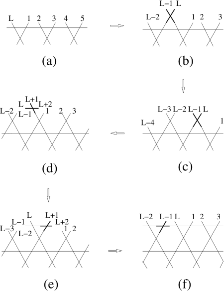
Figure 6: Constructing the transfer matrix. Appending a new row to the configuration is achieved in two parts. The first part consists of $L/2$ steps and is denoted $T_{L/2}\ldots T_{1}$ (which are executed from right to left). Each step adds a new site to the lattice. Two of these steps are illustrated in (a) to (c). The number of dangling bonds does not change during these steps. The second part consists of $L$ steps and is denoted $T_{3L/2}\ldots T_{L/2+1}$. The first step of these, $T_{L/2+1}$, adds a new vertex to the sub-row and increases the number of dangling bonds by 2 as shown in (d). The following steps $T_{L/2+2}\cdots T_{3L/2-1}$ append vertices sequentially, and do not change the number of dangling bonds. After adding the last vertex by $T_{3L/2}$ to the sub-row, the construction of a new row has been completed and the size of the system shrinks from $L+2$ to $L$.

While the construction of the transfer matrix is formulated in terms of connectivities on the topmost rows $M$ and $M+1$, the connectivity on row 1 is not entirely negligible. In particular, the number of dangling loop segments on that row can be even or odd. As a consequence the number of dangling loop segments on the topmost row is then also even or odd respectively. This leads to a decomposition of the transfer matrix in an even and an odd sector. The odd sector corresponds with a single loop segment running in the length direction of the cylinder.

IV.2 Results of the numerical calculation

For a model on an infinitely long cylinder with finite size $L$, the free energy per unit of area is determined by

$$f(L)=\frac{1}{\sqrt{3}L}\ln\Lambda_{L}^{(0)}\,,$$ (34)

where $\Lambda_{L}^{(0)}$ is the largest eigenvalue of $T$ in the $n_{d}=0$ sector. From the finite-size data for $f(L)$ we estimated the conformal anomaly $c$ BCN .

The magnetic correlation length $\xi_{h}(L)$ is related to the magnetic gap in the eigenvalue spectrum of $T$ as

$$\xi_{h}^{-1}(L)=\frac{1}{\sqrt{3}}\ln(\Lambda_{L}^{(0)}/\Lambda_{L}^{(1)})\,,$$ (35)

where $\Lambda_{L}^{(1)}$ is the largest eigenvalue of $T$ in the $n_{d}=1$ sector.

The temperature correlation length $\xi_{t}(L)$ is related to the temperature gap in the eigenvalue spectrum of $T$ as

$$\xi_{t}^{-1}(L)=\frac{1}{\sqrt{3}}\ln(\Lambda_{L}^{(0)}/\Lambda_{L}^{(2)})\,,$$ (36)

where $\Lambda_{L}^{(2)}$ is the second largest eigenvalue of $T$ in the $n_{d}=0$ sector. Using Cardy’s conformal mapping Cardy-xi of an infinite cylinder on the infinite plane, one can thus estimate the temperature dimension $X_{t}$ and $X_{h}$.

We calculated the finite-size data for the free energies of the FPL model at the critical points given by Eq. (20) for system sizes $L=2,~{}4,~{}\cdots,~{}28$. These data include the case $n=0$; this is possible because, for $q\to 0$ one has $u_{\rm hc}^{\rm c}=\sqrt{3q}$, so that the ratio between $a_{1}^{\rm c}$ and $a_{2}^{\rm c}$ in Eq. (20) remains well defined in this limit.

The additional loop configurations allowed by the dilute model lead to a larger transfer matrix for a given system size, so that our results at the critical points given by Eqs. (21) are restricted to sizes $L=2,~{}4,~{}\cdots,~{}18$. The latter results also include the temperature and magnetic gaps.

The finite-size data for the FPL and DL models displayed a good apparent convergence, and were fitted using methods explained earlier BNFSS ; BN ; GNB , see also Ref. FSS .

In the kagome lattice FPL model, it is not possible to introduce one single open loop segment running in the length direction of the cylinder. The presence of a single chain would force unoccupied edges into the system, in violation of the FPL condition. Therefore, we have no results for $X_{h}$. Furthermore, in the case of the low-temperature O($n$) phase, the eigenvalue associated with $X_{t}$ decreases rapidly when $n$ becomes smaller than 2, and becomes dominated by other eigenvalues. Therefore, also results for $X_{t}$ are absent for the FPL model, and our results are here restricted to the conformal anomaly $c$. The resulting estimates for the FPL model are listed in Tab. 1.

Table 1: Conformal anomaly $c$ of the FPL model as determined by the transfer-matrix calculations described in the text. The sizes of the system $L$ are from $2$ to $28$. Estimated error margins in the last decimal place are given in parentheses. The numerical results are indicated by ‘num’. For comparison, we include theoretical values indicated by ‘th’, as given by Eq. (23).

$n$	$c^{\rm th}$	$c^{\rm num}$
$0$	$-2$	$-2.000001$ (1)
$0.25$	$-1.3526699$	$-1.352670$ (5)
$0.5$	$-0.8197365$	$-0.819737$ (5)
$0.75$	$-0.3749081$	$-0.374908$ (5)
$1$	$0$	$0$
$1.25$	$0.31782377$	$0.31782$ (2)
$\sqrt{2}$	$1/2$	$0.5000000$ (2)
$1.50$	$0.58757194$	$0.587565$ (5)
$\sqrt{3}$	$4/5$	$0.80000$ (1)
$1.75$	$0.81497930$	$0.81498$ (2)
$2$	$1$	$1.0001$ (1)

The results for the eigenvalue $\Lambda_{L}^{(0)}$ of the the FPL model satisfy, within the numerical precision in the order of $10^{-12}$, the relation between the FPL and DL models derived in Sec. II.2. The larger dimensionality of the transfer matrix of the DL model in comparison with the FPL model generates new eigenvalues, and thus leads to new scaling dimensions that are absent in the FPL model. Final estimates for the conformal anomaly $c$ and for the scaling dimensions $X_{t}$ and $X_{h}$ are listed in Tab. 2 for the DL model. They agree well with the theoretical predictions, which are included in the table. Here we recall that, in analogy with the case of the branch-$0$ O($n$) loop model on the square lattice BN , the magnetic scaling dimension should be exactly equal to the thermal one. This is in agreement with our numerical results. We found that the eigenvalues $\Lambda_{L}^{(1)}$ and $\Lambda_{L}^{(2)}$ were the same within the numerical error margin. Thus, we list only one column with results for the exponents in Tab. 2.

Table 2: Conformal anomaly $c$, magnetic scaling dimension $X_{h}$ and temperature scaling dimension $X_{t}$ of the DL model as determined by the transfer-matrix calculations described in the text. Estimated error margins in the last decimal place are given in parentheses. The numerical results are indicated by ‘num’. For comparison, we include the theoretical values indicated by ‘th’, as given by Eqs. (24) and (26).

$n$	$c^{\rm th}$	$c^{\rm num}$	$X_{h}^{\rm th}$, $X_{t}^{\rm th}$	$X_{h}^{\rm num}$, $X_{t}^{\rm num}$
$-1$	$-2$	$-2.0000$ (5)	$0$	$0.0000000$ (1)
$-0.75$	$-1.3526699$	$-1.3524$ (3)	$0.073890718$	$0.0738908$ (2)
$-0.5$	$-0.8197365$	$-0.8194$ (5)	$0.138570601$	$0.138571$ (1)
$-0.25$	$-0.3749081$	$-0.3747$ (3)	$0.196602972$	$0.196605$ (5)
$0$	$0$	$0$	$1/4$	$0.25000$ (1)
$0.25$	$0.31782377$	$0.31778$ (5)	$0.300602502$	$0.30061$ (5)
$\sqrt{2}-1$	$1/2$	$0.500001$ (1)	$1/3$	$0.33334$ (1)
$0.50$	$0.58757194$	$0.5876$ (1)	$0.350604267$	$0.35061$ (1)
$\sqrt{3}-1$	$4/5$	$0.8002$ (3)	$2/5$	$0.3997$ (5)
$0.75$	$0.81497930$	$0.8151$ (3)	$0.404150985$	$0.4037$ (5)
$1$	$1$	$1.002$ (3)	$1/2$	$0.48$ (3)

V conclusion

We found a branch of critical points of the dilute loop model on the kagome lattice as a function of the loop weight $n$, which is related to the $q=(n+1)^{2}$-state Potts model on the honeycomb lattice. The critical properties of these critical points are conjectured and verified by numerical transfer matrix calculations and a finite-size-scaling analysis. As expected, the model falls into the same universality class as branch $0$ of the O($n$) loop model BN on the square lattice. The analysis did, however, yield a difference. This is due to the geometry of the lattice. For the square lattice, it was found BN that there exists a magnetic scaling dimension $X_{\rm int,1}$ as revealed by the free-energy difference between even and odd systems. Such an alternation is absent in the free-energy of the present model on the kagome lattice. While the number of dangling edges may be odd or even for the square lattice, it can only be even in the present case of the kagome lattice.

The numerical accuracy of the results for the conformal anomaly and the exponents is much better than what can be typically achieved for an arbitrary critical point, whose location in the parameter space has to be determined in advance by so-called phenomenological renormalization MPN . This seems not only due to the limited precision of such a critical point. We suppose that the main reason is that irrelevant scaling fields tend to be suppressed in exactly solvable parameter subspaces.

- (1) B. Nienhuis, Phys. Rev. Lett. 49, 1062 (1982); J. Stat. Phys. 34, 731 (1984).
- (2) E. Domany, D. Mukamel, B. Nienhuis and A. Schwimmer, Nucl. Phys. B 190 [FS3], 279 (1981).
- (3) H. W. J. Blöte and B. Nienhuis, J. Phys. A 22, 1415 (1989).
- (4) Y. M. M. Knops, H. W. J. Blöte and B. Nienhuis, J. Phys. A 26, 495 (1993).
- (5) B. Duplantier and H. Saleur, Phys. Rev. Lett. 59, 539 (1987).
- (6) H. W. J. Blöte, M. T. Batchelor and B. Nienhuis, Physica A 251, 95 (1988).
- (7) W.-A. Guo, B. Nienhuis and H. W. J. Blöte, Int. J. Mod. Phys. C 10, 291 (1999); Phys. Rev. Lett. 96, 045704 (2006).
- (8) P. W. Kasteleyn and C. M. Fortuin, J. Phys. Soc. Jpn. 46 (Suppl.), 11 (1969); C. M. Fortuin and P. W. Kasteleyn, Physica (Amsterdam) 57, 536 (1972).
- (9) R. J. Baxter, S. B. Kelland, F. Y. Wu, J. Phys. A 9, 397 (1976).
- (10) I. Syôzi, Progr. Theor. Phys. 6, 306 (1951).
- (11) F. Y. Wu, Rev. Mod. Phys. 54, 235 (1982).
- (12) H. W. J. Blöte, J. L. Cardy and M. P. Nightingale, Phys. Rev. Lett. 56, 742 (1986).
- (13) I. Affleck, Phys. Rev. Lett. 56, 746 (1986).
- (14) B. Nienhuis, in Phase Transitions and Critical Phenomena, eds. C. Domb and J. L. Lebowitz (Academic Press, London, 1987), Vol. 11.
- (15) D. Friedan, Z. Qiu and S. Shenker, Phys. Rev. Lett. 52, 1575 (1984).
- (16) H. W. J. Blöte and M. P. Nightingale, Physica A 112, 405 (1982).
- (17) J. L. Cardy, J. Phys. A 17, L385 (1984).
- (18) For reviews, see e.g. M. P. Nightingale in Finite-Size Scaling and Numerical Simulation of Statistical Systems, ed. V. Privman (World Scientific, Singapore 1990), and M. N. Barber in Phase Transitions and Critical Phenomena, eds. C. Domb and J. L. Lebowitz (Academic, New York 1983), Vol. 8.
- (19) M. P. Nightingale, Proc. Kon. Ned. Ak. Wet. B 82, 235 (1979).