Sivers Effect for Pion and Kaon Production in
Semi-Inclusive Deep Inelastic Scattering

Abstract

We study the Sivers effect in the transverse single spin asymmetries (SSA) for pion and kaon production in semi-inclusive deep inelastic scattering (SIDIS) processes. We perform a fit of $A^{\sin(\phi_{h}-\phi_{S})}_{UT}$ which, by including recent high statistics experimental data for pion and kaon production from HERMES and COMPASS Collaborations, allows a new determination of the Sivers distribution functions for quarks and antiquarks with $u$, $d$ and $s$ flavours. Estimates for forthcoming SIDIS experiments at COMPASS and JLab are given.

I Introduction

In Refs. Anselmino et al. (2005a, b), we studied the transverse single spin asymmetry $A_{UT}^{\sin(\phi_{h}-\phi_{S})}$ observed by the HERMES Airapetian et al. (2005) and COMPASS Alexakhin et al. (2005) Collaborations in polarized SIDIS processes, $\ell\,p\,(\mbox{\boldmath$S$})\to\ell^{\prime}\,h\,X$. The quality and amount of the data allowed to perform a rather well constrained extraction of the Sivers distribution function Sivers (1990, 1991) for $u$ and $d$ quarks, assuming the existence of a symmetric and negligibly small Sivers sea. Similar analyses and extractions were performed by other groups Vogelsang and Yuan (2005); Collins et al. (2006); Anselmino et al. (????). Although all these results were relevant and significant as the first determination of the Sivers $u$ and $d$ functions, they were affected by the low statistics of the experimental data available at that time: in fact, COMPASS asymmetries were limited to charged hadron production, as no hadron separation was performed, while the HERMES data were only given for charged pion production. Recently, much higher statistics data on the $A_{UT}^{\sin(\phi_{h}-\phi_{S})}$ azimuthal asymmetries for SIDIS have become available: in Ref. Diefenthaler (2007) the HERMES Collaboration presents neutral pion and charged kaon azimuthal asymmetries, in addition to higher precision data on charged pion asymmetries; moreover, Refs. Martin (2006); Alekseev et al. (2008) show the COMPASS Collaboration measurements for separated charged pion and kaon asymmetries, together with some data for $K^{0}_{S}$ production.

It is then timely and natural to reconsider the analysis performed in Ref. Anselmino et al. (2005b) in order to increase our understanding of the properties of the Sivers function. In particular, reduced error bars and hadron separation in both the HERMES and COMPASS sets of experimental data allow a better determination of the $u$ and $d$ flavour Sivers distribution functions and, most importantly, a first insight into the sea and strange contributions to the Sivers functions, namely $\Delta^{N}\!f_{\bar{u}/p^{\uparrow}}$, $\Delta^{N}\!f_{\bar{d}/p^{\uparrow}}$, $\Delta^{N}\!f_{s/p^{\uparrow}}$ and $\Delta^{N}\!f_{\bar{s}/p^{\uparrow}}$.

Our strategy is the following. First we evaluate the impact of the new data with respect to the old data sets: as we shall explain in Section III, using the same unpolarized fragmentation functions as in Refs. Anselmino et al. (2005a, b) would give a high quality fit as far as pion asymmetries are concerned, but fails to describe the kaon data. Instead, the use of a different, more recent set of fragmentation functions de Florian et al. (2007), based on a global analysis of pion and kaon production, will prove to be crucial to reach a successful description of pion and kaon data simultaneously. With a simple ansatz parameterization of the Sivers functions, we will then perform a simultaneous fit of both HERMES and COMPASS data sets on $A^{\sin(\phi_{h}-\phi_{S})}_{UT}$ for pion ($\pi^{\pm},\,\pi^{0}$) and $K^{\pm}$ production. We do not include in our fit the COMPASS data on $K^{0}_{S}$ Alekseev et al. (2008) as the corresponding fragmentation functions are not so well established and can be obtained from those for $K^{\pm}$ only adopting further assumptions; we shall rather estimate $A^{\sin(\phi_{h}-\phi_{S})}_{UT}$ for $K^{0}_{S}$, and compare it with COMPASS data, using the Sivers functions obtained by fitting all other data sets, and assuming exact $SU(2)$ invariance to derive the quark fragmentation functions into $K^{0}_{S}$.

The above procedure will allow to determine the valence and sea proton Sivers functions, which will be used to provide estimates for the analogous single spin asymmetries that will soon be measured at JLab (operating on proton, neutron and deuteron targets) and at COMPASS (operating on a proton target). Notice that the JLab measurements will provide vital information on the large $x$ behaviour of the Sivers distribution functions, yet undetermined from present SIDIS experiments, as explained in Section IV.

II Formalism and parameterization

The SIDIS transverse single spin asymmetry (SSA) $A^{\sin(\phi_{h}-\phi_{S})}_{UT}$ measured by HERMES and COMPASS is defined as (see Fig. 1 for the definition of the azimuthal angles)

$$A^{\sin(\phi_{h}-\phi_{S})}_{UT}=2\,\frac{\int d\phi_{S}\,d\phi_{h}\,[d\sigma^{\uparrow}-d\sigma^{\downarrow}]\,\sin(\phi_{h}-\phi_{S})}{\int d\phi_{S}\,d\phi_{h}\,[d\sigma^{\uparrow}+d\sigma^{\downarrow}]}\,,$$ (1)

and shows the azimuthal modulation triggered by the correlation between the nucleon spin and the quark intrinsic transverse momentum. This effect is embodied in the Sivers distribution function $\Delta^{N}\!f_{q/p^{\uparrow}}(x,k_{\perp})$, which appears in the number density of unpolarized quarks $q$ with intrinsic transverse momentum $\mbox{\boldmath$k$}_{\perp}$ inside a transversely polarized proton $p^{\uparrow}$, with three-momentum $P$ and spin polarization vector $S$,

$$\hat{f}_{q/p^{\uparrow}}(x,\mbox{\boldmath$k$}_{\perp}) = f_{q/p}(x,k_{\perp})+\frac{1}{2}\,\Delta^{N}\!f_{q/p^{\uparrow}}(x,k_{\perp})\;{\mbox{\boldmath$S$}}\cdot(\hat{\mbox{\boldmath$P$}}\times\hat{\mbox{\boldmath$k$}}_{\perp})\,,$$ (2)

where $f_{q/p}(x,k_{\perp})$ is the unpolarized $x$ and $k_{\perp}$ dependent parton distribution, and the mixed product ${\mbox{\boldmath$S$}}\cdot(\hat{\mbox{\boldmath$P$}}\times\hat{\mbox{\boldmath$k$}}_{\perp})$ explicitly gives the azimuthal dependence mentioned above. Notice that the Sivers function is also often denoted as $f_{1T}^{\perp q}(x,k_{\perp})$ Mulders and Tangerman (1996); this notation is related to ours by Bacchetta et al. (2004)

$$\Delta^{N}\!f_{q/p^{\uparrow}}(x,k_{\perp})=-\frac{2\,k_{\perp}}{m_{p}}\>f_{1T}^{\perp q}(x,k_{\perp})\>.$$ (3)

The “weighting” factor $\sin(\phi_{h}-\phi_{S})$ in Eq. (1) is appropriately chosen to single out, among the various azimuthal dependent terms appearing in $[d\sigma^{\uparrow}-d\sigma^{\downarrow}]$ Bacchetta et al. (2007); Anselmino et al. (2008), only the contribution of the Sivers mechanism. By properly taking into account all intrinsic motions this transverse single spin asymmetry can be written, at order $(k_{\perp}/Q)$, as Anselmino et al. (2005b)

$$A^{\sin(\phi_{h}-\phi_{S})}_{UT}=\frac{\displaystyle\sum_{q}\int{d\phi_{S}\,d\phi_{h}\,d^{2}\mbox{\boldmath$k$}_{\perp}}\;\Delta^{N}\!f_{q/p^{\uparrow}}(x,k_{\perp})\sin(\varphi-\phi_{S})\;\frac{d\hat{\sigma}^{\ell q\to\ell q}}{dQ^{2}}\;\;D_{q}^{h}(z,p_{\perp})\sin(\phi_{h}-\phi_{S})}{\displaystyle\sum_{q}\int{d\phi_{S}\,d\phi_{h}\,d^{2}\mbox{\boldmath$k$}_{\perp}}\;f_{q/p}(x,k_{\perp})\;\frac{d\hat{\sigma}^{\ell q\to\ell q}}{dQ^{2}}\;\;D_{q}^{h}(z,p_{\perp})}\>\cdot$$ (4)

$\phi_{S}$ and $\phi_{h}$ are the azimuthal angles identifying the directions of the proton spin $S$ and of the outgoing hadron $h$ respectively, while $\varphi$ defines the direction of the incoming (and outgoing) quark transverse momentum, $\mbox{\boldmath$k$}_{\perp}$ = $k_{\perp}(\cos\varphi,\sin\varphi,0)$, as shown in Fig. 1; $\frac{d\hat{\sigma}^{\ell q\to\ell q}}{dQ^{2}}$ is the unpolarized cross section for the elementary scattering $\ell q\to\ell q$,

$$\frac{d\hat{\sigma}^{\ell q\to\ell q}}{dQ^{2}}=e_{q}^{2}\,\frac{2\pi\alpha^{2}}{\hat{s}^{2}}\,\frac{\hat{s}^{2}+\hat{u}^{2}}{Q^{4}}\;,$$ (5)

where $\hat{s}$, $\hat{t}=-Q^{2}$ and $\hat{u}$ are the partonic Mandelstam invariants.

Finally, $D_{q}^{h}(z,p_{\perp})$ is the fragmentation function describing the hadronization of the final quark $q$ into the detected hadron $h$ with momentum $\mbox{\boldmath$P$}_{h}$ (see Fig. 1); $h$ carries, with respect to the fragmenting quark, a light-cone momentum fraction $z$ and a transverse momentum $\mbox{\boldmath$p$}_{\perp}$.

Figure 1: Kinematics of the SIDIS process in the $\gamma^{*}p$ center of mass frame.

In our analysis we shall consider $u$, $d$ and $s$ flavours for quarks and antiquarks. The Sivers function is parameterized in terms of the unpolarized distribution function, as in Ref. Anselmino et al. (2005b), in the following factorized form:

$$\Delta^{N}\!f_{q/p^{\uparrow}}(x,k_{\perp})=2\,{\cal N}_{q}(x)\,h(k_{\perp})\,f_{q/p}(x,k_{\perp})\;,$$ (6)

with

$${\cal N}_{q}(x)=N_{q}\,x^{\alpha_{q}}(1-x)^{\beta_{q}}\,\frac{(\alpha_{q}+\beta_{q})^{(\alpha_{q}+\beta_{q})}}{\alpha_{q}^{\alpha_{q}}\beta_{q}^{\beta_{q}}}\;,$$ (7)

$$h(k_{\perp})=\sqrt{2e}\,\frac{k_{\perp}}{M_{1}}\,e^{-{k_{\perp}^{2}}/{M_{1}^{2}}}\;,$$ (8)

where $N_{q}$, $\alpha_{q}$, $\beta_{q}$ and $M_{1}$ (GeV/$c$) are free parameters to be determined by fitting the experimental data. Since $h(k_{\perp})\leq 1$ for any $k_{\perp}$ and $|{\cal N}_{q}(x)|\leq 1$ for any $x$ (notice that we allow the constant parameter $N_{q}$ to vary only inside the range $[-1,1]$), the positivity bound for the Sivers function,

$$\frac{|\Delta^{N}\!f_{q/p^{\uparrow}}(x,k_{\perp})|}{2f_{q/p}(x,k_{\perp})}\leq 1\>,$$ (9)

is automatically fulfilled. We adopt the usual (and convenient) Gaussian factorization for the unpolarized distribution and fragmentation functions:

$$f_{q/p}(x,k_{\perp})=f_{q}(x)\,\frac{1}{\pi\langle k_{\perp}^{2}\rangle}\,e^{-{k_{\perp}^{2}}/{\langle k_{\perp}^{2}\rangle}}$$ (10)

and

$$D_{q}^{h}(z,p_{\perp})=D_{q}^{h}(z)\,\frac{1}{\pi\langle p_{\perp}^{2}\rangle}\,e^{-p_{\perp}^{2}/\langle p_{\perp}^{2}\rangle}\>,$$ (11)

with the values of $\langle k_{\perp}^{2}\rangle$ and $\langle p_{\perp}^{2}\rangle$ fixed to the values found in Ref. Anselmino et al. (2005a) by analysing the Cahn effect in unpolarized SIDIS:

$$\langle k_{\perp}^{2}\rangle=0.25\;({\rm GeV}/c)^{2}\quad\quad\quad\langle p_{\perp}^{2}\rangle=0.20\;({\rm GeV}/c)^{2}\>.$$ (12)

Notice that the Gaussian distributions limit the effective action of intrinsic motion to $k_{\perp}\mathrel{\hbox to0.0pt{\lower 4.0pt\hbox{\hskip 1.0pt$\sim$}\hss}\raise 1.0pt\hbox{$<$}}\sqrt{\langle k_{\perp}^{2}\rangle}$ and $p_{\perp}\mathrel{\hbox to0.0pt{\lower 4.0pt\hbox{\hskip 1.0pt$\sim$}\hss}\raise 1.0pt\hbox{$<$}}\sqrt{\langle p_{\perp}^{2}\rangle}$, which is the region of validity of the TMD factorized expressions in Eq. (4), $P_{T}\simeq k_{\perp}\simeq\Lambda_{\rm QCD}\ll Q$ Ji et al. (2005, 2004, 2006).

The parton distribution functions (PDF) $f_{q}(x)$ and the fragmentation functions (FF) $D_{q}^{h}(z)$ also depend on $Q^{2}$ via the usual QCD evolution, which will be taken into account, at leading order (LO), in all our computations.

Before fitting the data on the Sivers asymmetries a few comments on the quark hadronization are necessary. While most of the available sets of fragmentation functions describe rather well the pion multiplicities observed at HERMES, many of them fail to reproduce the kaon multiplicities in SIDIS production. The main reason is the role of the strange quarks, which is often not well established: for example, one expects that $K^{+}$ mesons can be abundantly produced by $\bar{s}$ quarks, via creation from the vacuum of a light $u\bar{u}$ pair, rather than by $u$ quarks, via creation from the vacuum of a heavier $s\bar{s}$ pair. Such a feature is particularly emphasized in the set recently obtained by de Florian, Sassot, Stratmann (DSS) de Florian et al. (2007), which has $D_{\bar{s}}^{K^{+}}(z)\,\gg\,D_{u}^{K^{+}}(z)$ over the whole $z$ range. This is shown in Fig. 2, where the LO DSS fragmentation functions (solid lines) are compared with those proposed by Kretzer (KRE) Kretzer (2000) (dashed lines) and by Hirai, Kumano, Nagai and Sudoh (HKNS) Hirai et al. (2007) (dotted lines). The DSS set, which is determined by fitting all presently available multiplicity measurements, both for pions and kaons, is indeed the most suitable for our purposes.

This can also be seen in a more quantitative way. We know that Kretzer’s and other commonly adopted sets of fragmentation functions are able to describe pion production data, as shown, for instance, in Fig. 4 of Ref. de Florian et al. (2007). However, Fig. 13 of Ref. de Florian et al. (2007) shows instead that Kretzer fragmentation functions fail to reproduce charged kaon SIDIS multiplicities, and might not be adequate to reconstruct transverse single spin asymmetries corresponding to kaon production. In fact, by using the Kretzer set for our fit, we would not be able to describe the kaon asymmetry data: to be more precise, we would obtain $\chi^{2}/d.o.f.\equiv\chi^{2}_{dof}\simeq 1$ for pions but $\chi^{2}_{dof}\simeq 4$ for kaon production asymmetries. Estimates for $K^{\pm}$ asymmetries were presented in Ref. Anselmino et al. (2005b) and the inadequacy of the Kretzer fragmentation functions was pointed out in several talks (see, for example, Ref. Prokudin et al. (Dubna, Russia, September 3-7, 2007)). The same conclusion has been confirmed, very recently, in Ref. Arnold et al. (2008).

Let us now turn to the experimental data on kaon and pion Sivers azimuthal asymmetries measured by the HERMES Collaboration Diefenthaler (2007). The single spin asymmetry corresponding to $K^{+}$ production is, as a matter of fact, much larger than the analogous asymmetry for $\pi^{+}$. Although one could naively expect, on the basis of $u$ quark dominance, that $K^{+}$ and $\pi^{+}$ asymmetries should be roughly the same, the presence of a large $D_{\bar{s}}^{K^{+}}$ FF can help to understand the “puzzle” of the $K^{+}$ asymmetry. Indeed, if a non-negligible $\bar{s}$ Sivers function exists, then its action combined with a large $D_{\bar{s}}^{K^{+}}$ fragmentation function can give rise to a significant difference between $K^{+}$ and $\pi^{+}$ Sivers asymmetries.

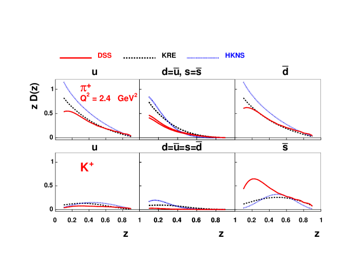
Figure 2: The LO unpolarized fragmentation functions for $u$, $d$ and $s$ flavours, at $Q^{2}=2.4$ (GeV/$c)^{2}$, as given by Kretzer Kretzer (2000) (dashed lines), by Hirai, Kumano, Nagai and Sudoh Hirai et al. (2007) (dotted lines) and by de Florian, Sassot and Stratmann de Florian et al. (2007) (solid lines). We show the fragmentation functions for $\pi^{+}$ in the upper panel, and for $K^{+}$ production in the lower panel. Notice that the fragmentation function describing the probability of a $K^{+}$ originating from an $\bar{s}$ quark is much larger than that associated to a $K^{+}$ from a $u$ quark, over the whole $z$ range. The two solid curves in the central upper plot correspond to $zD_{d}^{\pi^{+}}=zD_{\bar{u}}^{\pi^{+}}$ (upper line) and $zD_{s}^{\pi^{+}}=zD_{\bar{s}}^{\pi+}$ (lower line).

III Fit of SIDIS data and extraction of Sivers functions

The recent SIDIS experimental data on Sivers asymmetries for pion and kaon production give us the opportunity to study sea-quark Sivers functions for $\bar{u}$, $\bar{d}$, $s$ and $\bar{s}$ quarks. The $u$ and $d$ quark Sivers functions alone were already studied in Ref. Anselmino et al. (2005b); in the present analysis we will be able to improve the extraction of these functions and to present first estimates of the sea-quark Sivers functions.

In order to evaluate the significance of the sea-quark Sivers contributions we first perform a fit of the SIDIS data using flavour independent ratios of the sea-quark Sivers functions with the corresponding unpolarized PDFs: that is, for $\bar{u}$, $\bar{d}$, $s$ and $\bar{s}$ flavours we attempt an “unbroken sea” ansatz:

$$\Delta^{N}\!f_{q/p^{\uparrow}}(x,k_{\perp})=2\,{\cal N}_{sea}(x)\,h(k_{\perp})\,f_{q/p}(x,k_{\perp})\;,$$

$${\cal N}_{sea}(x)=N_{sea}\,x^{\alpha_{sea}}(1-x)^{\beta_{sea}}\,\frac{(\alpha_{sea}+\beta_{sea})^{(\alpha_{sea}+\beta_{sea})}}{\alpha_{sea}^{\alpha_{sea}}\beta_{sea}^{\beta_{sea}}}\;,$$ (13)

where $N_{sea},\alpha_{sea},\beta_{sea}$ are the same for all sea quarks, $q=\bar{u}$, $\bar{d}$, $s$ and $\bar{s}$.

As the SIDIS data from HERMES and COMPASS have a limited coverage in $x$, typically $x<0.3-0.4$, the experimental asymmetries we are fitting contain very little information on the large $x$ tail of the Sivers functions. In fact, our previous analysis of Ref. Anselmino et al. (2005b) showed that the parameters $\beta_{u}$ and $\beta_{d}$ as determined by MINUIT best fit procedure are affected by very large errors. Therefore, as a first attempt, we assume the same value of $\beta$ for all Sivers functions, setting $\beta_{sea}=\beta_{u}=\beta_{d}\equiv\beta$.

Thus for the “unbroken sea” ansatz we have 8 free parameters:

$$N_{u}\quad\quad\quad N_{d}\quad\quad\quad N_{sea}$$

$$\alpha_{u}\quad\quad\quad\,\alpha_{d}\quad\quad\quad\;\alpha_{sea}$$ (14)

$$\beta\quad\quad\quad\,\,\,M_{1}\;({\rm GeV}/c)\>.$$

For the purposes of our fit, we use the unpolarized parton distribution functions $f_{q}(x,Q^{2})$ as given in Ref. Gluck et al. (1998) (GRV98LO) and the fragmentation functions $D_{q}^{h}(z,Q^{2})$ as given in Ref. de Florian et al. (2007) (DSS) – all evolved to the appropriate $Q^{2}$ values – with the additional $k_{\perp}$ Gaussian dependences of Eqs. (10)-(12). While the choice of the DSS fragmentation functions is the one which best describes the large asymmetries observed for $K^{+}$, the use of different sets of distribution functions, including the most recent analysis of $s$ quark distributions from HERMES Airapetian et al. (2008), would not affect our results significantly. For the Sivers functions, we use the functional forms of Eqs. (6)-(8). Notice that the (unknown) $Q^{2}$ evolution of these functions is assumed to be the same as for the unpolarized PDFs, $f_{q}(x,Q^{2})$.

By fitting simultaneously pion and kaon production data from HERMES Diefenthaler (2007) and COMPASS Martin (2006) we obtain an acceptable overall description of the experimental data, with $\chi^{2}_{dof}=1.16$. The new experimental data give clear indications of the need of a non negligible sea-quark Sivers function, with $N_{sea}=-0.13\pm 0.03$ sensitively different from zero. Although the total $\chi^{2}_{dof}$ is definitely good, a more careful examination of the results shows that while we achieve a perfect description of the $\pi^{+}$ production data at HERMES Diefenthaler (2007), with $\chi^{2}\simeq 1$ per data point, the description of kaon production data is rather poor, with $\chi^{2}\simeq 3$ per data point for $K^{+}$ production at HERMES Diefenthaler (2007). This indicates that the “unbroken sea” ansatz fails to reproduce the differences between pion and kaon production, and clearly suggests the need of a parameterization which should allow for a more structured flavour dependence of the sea-quark Sivers functions.

Including four new functions in our analysis would result in a substantial growth of the number of parameters and would consequently limit the usefulness of our parameterization. To keep the number of parameters under control, we define a simple “broken sea” ansatz by introducing four free parameters, $N_{\bar{u}}$, $N_{\bar{d}}$, $N_{s}$, and $N_{\bar{s}}$ which give different sizes to the sea-quark Sivers functions, while keeping the same functional forms ($\alpha_{\bar{u}}=\alpha_{\bar{d}}=\alpha_{s}=\alpha_{\bar{s}}\equiv\alpha_{sea}$ and $\beta_{sea}=\beta_{u}=\beta_{d}\equiv\beta$). For the “broken sea” ansatz fit we then have 11 parameters:

$$N_{u}\quad\quad\quad N_{d}\quad\quad\quad N_{s}$$

$$N_{\bar{u}}\quad\quad\quad N_{\bar{d}}\quad\quad\quad N_{\bar{s}}$$

$$\alpha_{u}\quad\quad\quad\,\alpha_{d}\quad\quad\quad\;\alpha_{sea}$$ (15)

$$\beta\quad\quad\quad\,\,\,M_{1}\;({\rm GeV}/c)\>.$$

The results we obtain for these parameters by fitting simultaneously the four experimental data sets on $A_{UT}^{\sin(\phi_{h}-\phi_{S})}$, corresponding to pion and kaon production at HERMES Diefenthaler (2007) and COMPASS Martin (2006), are presented in Table 1, together with the corresponding errors, estimated according to the procedure outlined in Appendix A. The fit performed under the “broken sea” ansatz shows a remarkable improvement, especially concerning the description of kaon data. We now obtain $\chi^{2}=1.20$ per data point for $K^{+}$ production at HERMES Diefenthaler (2007), while for pions we have $\chi^{2}=0.94$ per data point, and a total $\chi^{2}_{dof}=1.00$. In Table II we show the $\chi^{2}$ per data point for pion and kaon production at HERMES and COMPASS, both for the ”unbroken sea” and ”broken sea” ansatze and adopting the Kretzer and DSS FF sets. Notice that these values refer to the asymmetries as a function of $x$.

The quality of our results is shown in Figs. 3 and 4 where our best fit to the SSA is compared with the experimental data from Refs. Diefenthaler (2007) and Martin (2006): the SSAs are plotted as a function of one variable at a time, either $x$ or $z$ or $P_{T}$, while an integration over the other variables has been performed consistently with the cuts of the corresponding experiment.

Table 1: Best values of the free parameters for the “broken sea” ansatz, Eq. (15). Notice that the statistical errors reported in this table are not the errors given by MINUIT. As the parameters are strongly correlated, we determine them according to the procedure explained in Appendix A. The significant fluctuations in our results are shown by the shaded areas in Figs. 3 and 4.

$\chi^{2}/d.o.f.=1.00$
$N_{u}=0.35^{+0.08}_{-0.08}$	$N_{d}=-0.90^{+0.43}_{-0.10}$	$N_{s}=-0.24^{+0.62}_{-0.50}$
$N_{\bar{u}}=0.04^{+0.22}_{-0.24}$	$N_{\bar{d}}=-0.40^{+0.33}_{-0.44}$	$N_{\bar{s}}=1^{+0}_{-0.0001}$
$\alpha_{u}=0.73^{+0.72}_{-0.58}$	$\alpha_{d}=1.08^{+0.82}_{-0.65}$	$\alpha_{sea}=0.79^{+0.56}_{-0.47}$
$\beta\;\;=3.46^{+4.87}_{-2.90}$	$M_{1}^{2}=0.34^{+0.30}_{-0.16}$ (GeV/$c)^{2}$

Table 2: $\chi^{2}$ per data point for pion and kaon production at HERMES and COMPASS, both for the “unbroken sea” and “broken sea” ansatze, and adopting the Kretzer and DSS FF sets. $x$ dependent data, integrated over $z$ and $P_{T}$, are considered here.

Experiment	observed hadron	n. of data points	$\chi^{2}$ per data point
			Kretzer		DSS
			unbroken sea	broken sea	unbroken sea	broken sea
	$\pi^{+}$	5	$0.65$	$0.53$	$0.57$	$0.56$
	$\pi^{-}$	5	$2.67$	$2.64$	$1.60$	$1.62$
HERMES	$\pi^{0}$	5	$0.48$	$0.46$	$0.47$	$0.43$
	$K^{+}$	5	$6.14$	$5.71$	$3.87$	$2.11$
	$K^{-}$	5	$0.79$	$0.80$	$0.73$	$0.69$
	$\pi^{+}$	9	$0.65$	$0.57$	$0.39$	$0.64$
COMPASS	$\pi^{-}$	9	$0.83$	$0.55$	$0.49$	$0.70$
	$K^{+}$	9	$0.84$	$0.75$	$0.78$	$0.57$
	$K^{-}$	9	$1.47$	$1.34$	$1.17$	$1.36$

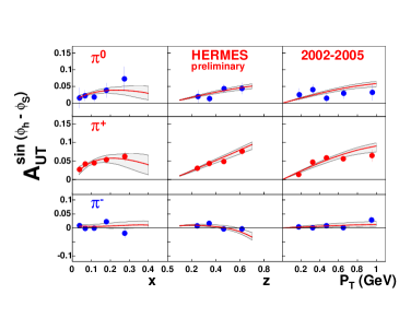
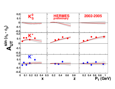
Figure 3: The results obtained from our simultaneous fit of the SIDIS $A_{UT}^{\sin{(\phi_{h}-\phi_{S})}}$ Sivers asymmetries (solid lines) are compared with HERMES experimental data Diefenthaler (2007) for pion and kaon production (left and right panel, respectively). The shaded area corresponds to the statistical uncertainty of the parameters, see Appendix A for further details. For completeness, we also show the $K_{S}^{0}$ asymmetry, not measured at HERMES, which is the result of a computation based on our extracted Sivers function and the assumed fragmentation functions of Eq. (16).

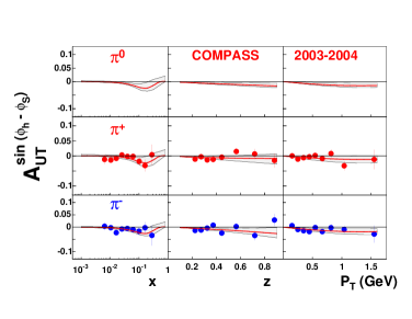
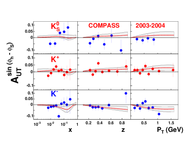
Figure 4: The results obtained from our fit (solid lines) are compared with the COMPASS measurements of $A_{UT}^{\sin{(\phi_{h}-\phi_{S})}}$ for pion (left panel) and kaon (right panel) production Martin (2006) off a deuteron target. The shaded area corresponds to the statistical uncertainty of the parameters, as explained in Appendix A. The $\pi^{0}$ asymmetry, not measured at COMPASS, is the result of a computation based on our extracted Sivers functions. Also the $K_{S}^{0}$ asymmetry, although compared with data Alekseev et al. (2008), is not a best fit, but the result of our computation, using the assumed fragmentation functions of Eq. (16).

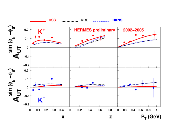
Figure 5: The results obtained from our fit using the kaon fragmentation functions as given by de Florian et al. in Ref. de Florian et al. (2007) (solid lines) are compared with the results we would find by using the KRE Kretzer (2000)(dotted lines) and HKNS Hirai et al. (2007) (dashed lines) sets of fragmentation functions.

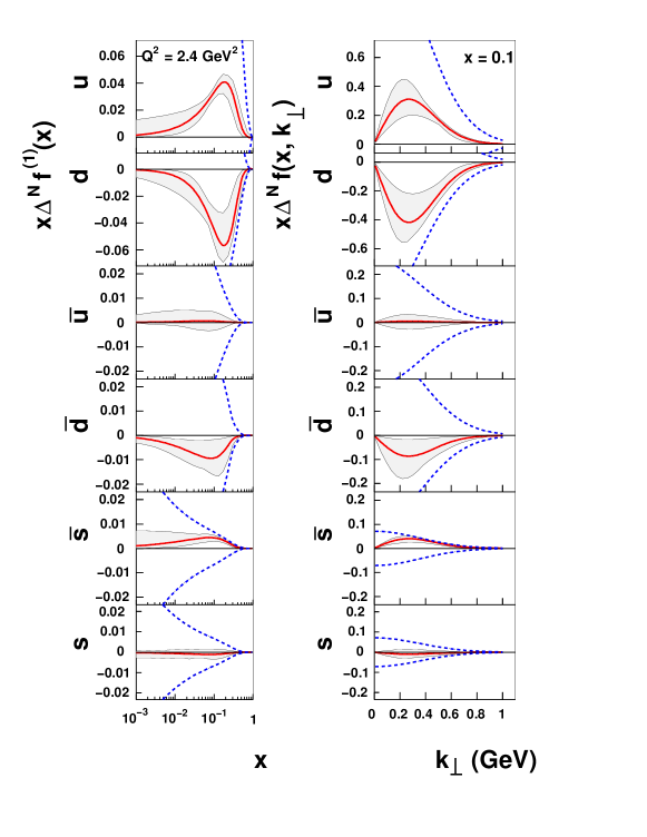
Figure 6: The Sivers distribution functions for $u$, $d$ and $s$ flavours, at the scale $Q^{2}=2.4$ (GeV$/c)^{2}$, as determined by our simultaneous fit of HERMES and COMPASS data (see text for details). On the left panel, the first moment $x\,\Delta^{N}\!f^{(1)}(x)$, Eq. (17), is shown as a function of $x$ for each flavour, as indicated. Similarly, on the right panel, the Sivers distribution $x\,\Delta^{N}\!f(x,k_{\perp})$ is shown as a function of $k_{\perp}$ at a fixed value of $x$ for each flavour, as indicated. The highest and lowest dashed lines show the positivity limits $|\Delta^{N}\!f|=2f$.

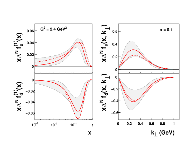
Figure 7: The Sivers distribution functions for $u$ and $d$ flavours, at the scale $Q^{2}=2.4$ (GeV$/c)^{2}$, as determined by our present fit (solid lines), are compared with those of our previous fit Anselmino et al. (2005b) of SIDIS data (dashed lines), where $\pi^{0}$ and kaon productions were not considered and only valence quark contributions were taken into account. This plot clearly shows that the Sivers functions previously found are consistent, within the statistical uncertainty bands, with the Sivers functions presently obtained.

In order to check the dependence on the set of unpolarized PDF’s adopted, we have also performed the fit by using the CTEQ6L Pumplin et al. (2002) and the MRST01LO Martin et al. (2002) sets; in both cases, the quality of the fit and the central-value results for the asymmetries are so similar to those obtained with the GRV98LO set that they would be hardly distinguishable in Figs. 3 and 4.

The shaded areas in Figs. 3 and 4 (and in all subsequent figures where they are shown) represent statistical uncertainties and correspond to a 95.45% Confidence Level (CL): they are determined according to the procedure described in Appendix A. Notice that further uncertainties of theoretical nature, intrinsic to our phenomenological approach, are present and might widen the size of the statistical bands. However, these are very difficult to assess: it suffices to recall that our analysis is performed assuming a simple factorized $k_{\perp}$ dependence in Eqs. (6), (10) and (11), that the actual $Q^{2}$ evolution of the Sivers function is unknown and that uncertainties in the fragmentation functions have not been taken into account. The functional form for the $x$-dependence of the Sivers functions used in the fit, Eq. (7), is a simple one and more structured dependences might allow better fits, with the statistical shaded areas covering better the experimental errors of the data. At this stage, considering the available experimental information and the remaining theoretical issues to be clarified, we do not think that further refinements of our analysis would be meaningful.

Notice that in Fig. 4 we also show the results for $\pi^{0}$ at COMPASS, for which no data is so far available, computed using our extracted Sivers functions as given in Table 1. Similarly we have computed $A_{UT}^{\sin(\phi_{h}-\phi_{S})}$ for $K^{0}_{S}$ production at HERMES and COMPASS and show them respectively in Figs. 3 and 4. As the $K^{0}_{S}$ is an equal mixture of $K^{0}=d\bar{s}$ and $\bar{K}^{0}=\bar{d}s$, we have assumed isospin invariance, writing the $K^{0}_{S}$ FFs in terms of the $K^{+}$ ones – which are taken from Ref. de Florian et al. (2007) – as:

$$D_{d}^{K^{0}_{S}}=D_{\bar{d}}^{K^{0}_{S}}=\frac{1}{2}\left[D_{u}^{K^{+}}+D_{sea}^{K^{+}}\right]$$

$$D_{\bar{s}}^{K^{0}_{S}}=D_{s}^{K^{0}_{S}}=\frac{1}{2}\left[D_{\bar{s}}^{K^{+}}+D_{sea}^{K^{+}}\right]$$ (16)

$$D_{u}^{K^{0}_{S}}=D_{\bar{u}}^{K^{0}_{S}}=D_{sea}^{K^{+}}\equiv D_{d}^{K^{+}}=D_{\bar{u}}^{K^{+}}=D_{s}^{K^{+}}=D_{\bar{d}}^{K^{+}}\,.$$

Our computation of the $K^{0}_{S}$ asymmetry at COMPASS can be compared with the available data Alekseev et al. (2008), as shown in the upper-right plots of Fig. 4. Notice that these curves, contrary to the others in the same figure, are not best fits, but a simple estimate, based on the extracted Sivers functions and the adopted fragmentation functions of Eq. (16).

In Fig. 5, our results, obtained using the kaon fragmentation functions as given by de Florian et al. in Ref. de Florian et al. (2007) (solid lines), are compared with the best fit we would find by using the KRE Kretzer (2000) (dotted lines) and HKNS Hirai et al. (2007) (dashed lines) sets of fragmentation functions. It is clear that the use of the new – strange-quark sensitive – fragmentation functions yields a much better agreement with the experimental measurements of the SIDIS azimuthal asymmetries for kaon production.

The Sivers functions generated by our best fit procedure are presented, at the scale $Q^{2}=2.4$ (GeV$/c)^{2}$, in Fig. 6, where we plot, on the left panel, the first $\mbox{\boldmath$k$}_{\perp}$ moment defined as

$$\Delta^{N}\!f_{q/p^{\uparrow}}^{(1)}(x)\equiv\int d^{2}\,\mbox{\boldmath$k$}_{\perp}\,\frac{k_{\perp}}{4m_{p}}\,\Delta^{N}\!f_{q/p^{\uparrow}}(x,k_{\perp})=-f_{1T}^{\perp(1)q}(x)\>,$$ (17)

and, on the right panel, the $k_{\perp}$ dependence of $\Delta^{N}\!f_{q/p^{\uparrow}}$ at a fixed value of $x=0.1$. The highest and lowest dashed lines show the positivity limits $|\Delta^{N}\!f|=2f$.

Our results both confirm previous conclusions on the $u$ and $d$ Sivers distributions and, despite the still large uncertainties (see Table 1), offer some new clear information about the so far unknown sea-quark Sivers functions. Let us comment in detail:

• The HERMES data on kaon asymmetries, surprisingly large for $K^{+}$, cannot be explained without a sea-quark Sivers distribution. In particular, we definitely find

  $$\Delta^{N}\!f_{\bar{s}/p^{\uparrow}}>0$$ (18)

  and confirm the previous findings for valence flavours Anselmino et al. (2005b); Vogelsang and Yuan (2005); Collins et al. (2006); Anselmino et al. (????),

  $$\Delta^{N}\!f_{u/p^{\uparrow}}>0\quad\quad\quad\Delta^{N}\!f_{d/p^{\uparrow}}<0\>.$$ (19)

  There are simple reasons for the above results. The Sivers distribution function for $\bar{s}$ quarks turns out to be definitely positive, due to the large positive value of $A_{UT}^{\sin(\phi_{h}-\phi_{S})}$ for $K^{+}$; notice that the value of $N_{\bar{s}}$ saturates the positivity bound $|N_{q}|\leq 1$. Similarly, the positive sign of $\Delta^{N}\!f_{u/p^{\uparrow}}$ is, essentially, driven by the positive $\pi^{+}$ and $K^{+}$ SSAs and the opposite sign of $\Delta^{N}\!f_{d/p^{\uparrow}}$ by the small SSA measured by COMPASS on a deuteron target. The $u$ and $d$ Sivers functions are also predicted to be opposite in the large $N_{c}$ limit Pobylitsa (2003) and in chiral models Drago (2005).

• The Sivers functions for $\bar{u}$, $\bar{d}$ and $s$ quarks, instead, turn out to have much larger uncertainties; even the sign of the $\bar{u}$ and $s$ Sivers functions is not fixed by available data, while $\Delta^{N}\!f_{\bar{d}/p^{\uparrow}}$ appears to be negative. This could be consistent with a positive contribution from $u$ quarks, necessary to explain the large $K^{+}$ asymmetry, which is decreased, for $\pi^{+}$, by a negative $\bar{d}$ contribution. One might expect correlated Sivers functions for $s$ and $\bar{s}$ quarks: we have actually checked that choosing $\Delta^{N}\!f_{s/p^{\uparrow}}=\pm\Delta^{N}\!f_{\bar{s}/p^{\uparrow}}$ slightly worsens the $\chi^{2}_{dof}$ (from 1 up to about 1.1), but still leads to a reasonable fit.

• We notice that the Burkardt sum rule Burkardt (2004)

  $$\sum_{a}\int dx\,d^{2}\mbox{\boldmath$k$}_{\perp}\,\mbox{\boldmath$k$}_{\perp}\,f_{a/p^{\uparrow}}(x,\mbox{\boldmath$k$}_{\perp})\equiv\sum_{a}\,\langle\mbox{\boldmath$k$}_{\perp}^{a}\rangle=0\>,$$ (20)

  where, from Eqs. (2) and (17),

  $$\langle\mbox{\boldmath$k$}_{\perp}^{a}\rangle = \left[\frac{\pi}{2}\int_{0}^{1}\!\!dx\int_{0}^{\infty}\!\!dk_{\perp}\,k_{\perp}^{2}\,\Delta^{N}\!f_{a/p^{\uparrow}}(x,k_{\perp})\right](\mbox{\boldmath$S$}\times\hat{\mbox{\boldmath$P$}})$$ (21)

  $$= m_{p}\int_{0}^{1}\!\!dx\,\Delta^{N}\!f_{q/p^{\uparrow}}^{(1)}(x)\,(\mbox{\boldmath$S$}\times\hat{\mbox{\boldmath$P$}})\equiv\langle k_{\perp}^{a}\rangle\,(\mbox{\boldmath$S$}\times\hat{\mbox{\boldmath$P$}})\,,$$

  is almost saturated by $u$ and $d$ quarks alone at $Q^{2}=2.4$ (GeV$/c)^{2}$:

  $$\langle k_{\perp}^{u}\rangle+\langle k_{\perp}^{d}\rangle=-17^{+37}_{-55}\>\>({\rm MeV}/c)\quad\quad\quad\langle k_{\perp}^{\bar{u}}\rangle+\langle k_{\perp}^{\bar{d}}\rangle+\langle k_{\perp}^{s}\rangle+\langle k_{\perp}^{\bar{s}}\rangle=-14^{+43}_{-66}\>\>({\rm MeV}/c).$$ (22)

  The individual contributions for quarks are:

  $$\langle k_{\perp}^{u}\rangle = 96^{+60}_{-28}\>\>({\rm MeV}/c)\quad\quad\quad\langle k_{\perp}^{d}\rangle\,=-113^{+45}_{-51}\>\>({\rm MeV}/c)$$

  $$\langle k_{\perp}^{\bar{u}}\rangle = \>\>2^{+24}_{-11}\>\>({\rm MeV}/c)\quad\quad\quad\langle k_{\perp}^{\bar{d}}\rangle\,=\,\,\>-28^{+20}_{-60}\>\>({\rm MeV}/c)$$ (23)

  $$\langle k_{\perp}^{s}\rangle = \!\!-4^{+11}_{-15}\>\>({\rm MeV}/c)\quad\quad\quad\langle k_{\perp}^{\bar{s}}\rangle\,=\quad\>\,17^{+30}_{-8}\ ({\rm MeV}/c)\>,$$

  thus leaving little room for a gluon Sivers function,

  $$-10\leq\langle k_{\perp}^{g}\rangle\leq 48\ ({\rm MeV}/c)\>,$$ (24)

  in agreement with other similar results Anselmino et al. (2006); Brodsky and Gardner (2006). The statistical uncertainties in the values given above have been computed as explained at the end of Appendix A.

• In Fig. 7 we compare the $u$ and $d$ flavour Sivers distribution functions, at the scale $Q^{2}=2.4$ (GeV$/c)^{2}$, obtained in our present analysis with the $u$ and $d$ flavour Sivers functions we had found from our previous fit Anselmino et al. (2005b), where $\pi^{0}$ and kaon productions were not considered, the Kretzer fragmentation function set was used, and only valence quark contributions were taken into account in the polarized proton. This plot shows that the Sivers functions previously obtained are consistent, within the statistical uncertainty bands, with the Sivers functions presently found.

IV Estimates for forthcoming experiments

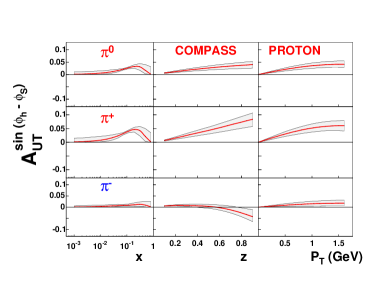
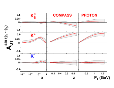
Figure 8: Estimates for the single spin asymmetry $A_{UT}^{\sin(\phi_{h}-\phi_{S})}$ for pion and kaon production off a hydrogen target, which will be measured by the COMPASS Collaboration.

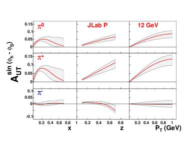
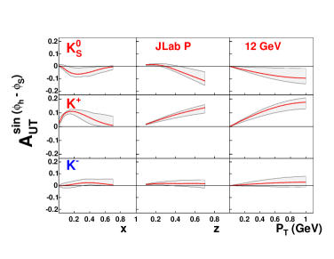
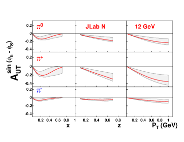
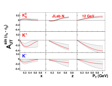
Figure 9: Estimates for the single spin asymmetry $A_{UT}^{\sin(\phi_{h}-\phi_{S})}$ for pion and kaon production, which will be measured at JLab operating on a polarized hydrogen target with a beam energy of $12$ GeV.

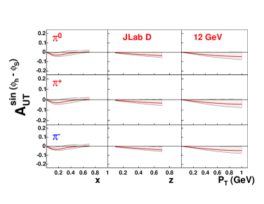
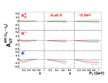
Figure 10: Estimates for the single spin asymmetry $A_{UT}^{\sin(\phi_{h}-\phi_{S})}$ for pion and kaon production, which will be measured at JLab operating on a polarized He³ (neutron) target, with a beam energy of $12$ GeV.

Figure 11: Estimates for the single spin asymmetry $A_{UT}^{\sin(\phi_{h}-\phi_{S})}$ for pion and kaon production at JLab off a polarized deuteron target, with a beam energy of $12$ GeV.

Using the Sivers functions determined through our fit, we can give estimates for other transverse single spin asymmetries $A_{UT}^{\sin(\phi_{h}-\phi_{S})}$ which will be measured in the near future. Fig. 8 shows the results we obtain for the COMPASS experiment operating with a hydrogen target, adopting the same experimental cuts which were used for the deuterium target (Eq. (71) of Ref. Anselmino et al. (2005a)).

Forthcoming measurements at the energies of $6$ and $12$ GeV are going to be performed at JLab, on transversely polarized proton, neutron and deuteron targets. The obtained data will be important for several reasons; they will cover a kinematical region corresponding to large values of $x$, a region which is so far unexplored by other SIDIS measurements. In particular, a combined analysis of HERMES, COMPASS and JLab SIDIS data will allow a much better determination of the $\beta$ parameters, which control the large $x$ behaviour of the Sivers distribution functions. In addition, the combined analysis of proton and neutron target events will help flavour disentangling and a more precise determination of $u$ and $d$ quark contributions.

Our estimates for the JLab SSAs, for pion and kaon production off proton, neutron and deuteron targets, at 12 GeV, are presented in Figs. 11–11. At this energy relatively large $Q^{2}$ values are available and the TMD factorization, valid for $P_{T}\simeq k_{\perp}\simeq\Lambda_{\rm QCD}\ll Q$, should hold. The adopted experimental cuts for a proton or a deuteron target are, in terms of the usual SIDIS variables, the following:

$$0.3\leq z_{h}\leq 0.8\;\;\;$$

(25)

whereas for a neutron target they are:

$$0.3\leq z_{h}\leq 0.7$$

(26)

where, at order $(k_{\perp}/Q)$, one has $x_{{}_{\!B}}=x$ and $z_{h}=z$; the exact relationships can be found in Ref. Anselmino et al. (2005a).

Notice that these estimates, while well constrained by the available SIDIS data at small $x$ values, might be less stringent at large $x$ values: for example, relaxing the assumption of a unique $\beta$ value for all flavours, would only marginally affect our present fit of HERMES and COMPASS data, but would much widen the uncertainty band above $x\simeq 0.4$.

We have given complete sets of estimates for charged and neutral pions and kaons. While the $\pi^{\pm},\,\pi^{0}$ and $K^{\pm}$ computations originate from a consistent procedure which uses fragmentation functions and Sivers distributions obtained by fitting data involving the same particles, the $K^{0}_{S}$ estimates might be affected by a greater uncertainty about its fragmentation functions, which require the assumptions of Eq. (16). This can be seen in the comparison between data and computations of Fig. 4.

We have also computed estimates for JLab operating at 6 GeV, with the corresponding kinematical cuts:

$$0.4\leq z_{h}\leq 0.7$$

(27)

for a proton or a deuteron target, and

$$0.46\leq z_{h}\leq 0.59$$

(28)

for a neutron target. The SSAs result to be almost identical to those obtained at 12 GeV; therefore, we do not show them explicitely.

A word of caution is necessary when discussing JLab SIDIS observables at 6 GeV; in the high-$x$, relatively low-$Q^{2}$ JLab kinematical regime, target and identified hadron mass effects (in particular for kaons), large $x$ resummations and higher-twist effects might be significant. This implies potential theoretical problems in the analysis of such data. Notice, moreover, that a much better statistics should be expected at 12 GeV.

V Conclusions

We have performed a comprehensive analysis of SIDIS data on Sivers azimuthal dependences, taking advantage of new and more precise experimental results. Particularly challenging are the HERMES data on kaon asymmetries, showing an unexpectedly large value of $A_{UT}^{\sin(\phi_{h}-\phi_{S})}$ for $K^{+}$. Our results confirm and improve previous extractions of the $u$ and $d$ Sivers distributions and offer first insights into the sea contribution to the Sivers effect.

It turns out that the data demand a non vanishing, and large, Sivers distribution for $\bar{s}$ quarks, which, coupled to a new set of fragmentation functions enhancing the role of strange quarks, appears to be the only way, at present, to explain the $K^{+}$ data. The other sea quark ($\bar{u},\bar{d},s$) contributions are, at this stage, less well determined, although they also seem to be non vanishing.

Taken at face value, the extracted Sivers distributions indicate a saturation of the Burkardt sum rule mainly due to $u$ and $d$ quarks alone, which carry almost opposite transverse momentum. The sea quark contribution is altogether rather small. This seems to rule out a contribution from gluons and, somehow, points towards a picture of the proton structure with the parton orbital motion restricted to valence quarks.

Finally, we have used our extracted Sivers distributions to compute estimates for ongoing and planned new experiments at COMPASS and JLab.

Appendix A $\chi^{2}$ analysis and statistical uncertainty bands

For completeness, and because it is often a matter of debate, we briefly discuss the techniques used for evaluating the statistical uncertainties of our estimates. A standard (see Refs. Yao et al. (2006), Press et al. (2007)) $\chi^{2}$ analysis is applied in order to estimate the values of $M$ unknown parameters ${\bf a}=\{a_{1},...,a_{M}\}$. The total $\chi^{2}$ is calculated by

$$\chi^{2}=\sum_{i=1}^{N}\left(\frac{y_{i}-F(x_{i};{\bf a})}{\sigma_{i}}\right)^{2},$$ (29)

where we have a set of $N$ experimental measurements $y_{i}$ at known points $x_{i}$. Each measurement is supposed to be Gaussian distributed with variance $\sigma_{i}^{2}$. The theoretical estimate $F(x_{i};{\bf a})$ of the measurement $y_{i}$ depends non-linearly on the $M$ unknown parameters $a_{i}$.

Minimizing the total $\chi^{2}$ yields a set of parameters ${\bf a}_{0}$ and a value $\chi^{2}_{min}=\chi^{2}({\bf a}_{0})$.

In our particular case we have $N=173$ and, for the “broken sea” ansatz, $M=11$, thus $n_{d.o.f.}=162$; the minimum $\chi^{2}$ found by MINUIT is $\chi^{2}_{min}=162.65$.

At this stage, we would like to estimate the possible errors on the extracted parameters and the statistical uncertainties on the corresponding Sivers functions and on our estimates for the asymmetries which will be measured in future experiments.

Let us call ${\bf a}_{j}$ some sets of parameters that could have been obtained if a slightly different set of data $\{x_{i},y_{i}\}_{j}$ were measured (within experimental uncertainties one can generate, using Monte Carlo techniques, new data sets and extract the corresponding parameter sets ${\bf a}_{j}$). Then, for each value of $j$, the quantity

$$\Delta\chi^{2}\equiv\chi^{2}({\bf a}_{j})-\chi^{2}({\bf a}_{0})$$ (30)

is distributed according to a chi-square distribution, with $M$ degrees of freedom (see sects. 32.3.2.3 of Ref. Yao et al. (2006), 15.6 of Ref. Press et al. (2007)). In order to take into account the correlations between all the parameters, we would like to perform a joint estimation of $M$ parameters. The corresponding coverage probability can be calculated according to the formula

$$\displaystyle P=\int_{0}^{\Delta\chi^{2}}\frac{1}{2\Gamma(M/2)}\left(\frac{\chi^{2}}{2}\right)^{(M/2)-1}\exp\left(-\frac{\chi^{2}}{2}\right){\rm d}\chi^{2}\,.$$ (31)

The meaning of the coverage probability can be explained as follows: suppose that we generate sets of parameters ${\bf a}_{j}$, $j=1,..,I$, which satisfy the condition

$$\chi^{2}({\bf a}_{j})\leq\chi^{2}_{min}+\Delta\chi^{2}\,;$$ (32)

then, if the number of sets is large enough, we cover a hyper-volume in the $M$ dimensional space which is called confidence region. The meaning of the confidence region is that with a probability $P$ we will find the true set of parameters ${\bf a}_{true}$ inside this hyper-volume (see sect. 15.6 of Press et al. (2007)). The minimal probability which is worth quoting is 68.3% and is historically connected to one sigma deviation of the normal distribution, then 95.45% corresponding to 2 sigma, etc.

Notice that if we wanted to estimate the error of one single parameter, say $a_{1}$, having fixed all the other parameter values, then the previous considerations would lead us back to the well known case in which $M=1$, and $\Delta\chi^{2}=1$ for a required 68.3% confidence level.

We determine the confidence hyper-volume corresponding to $P=0.9545$ coverage probability for the joint estimation of $M$ parameters. From Eq. (31), we obtain

$$\Delta\chi^{2}_{fit}=19.988\,.$$ (33)

We then generate 200 sets of parameters ${\bf a}_{j}$, $j=1,...,200$ which satisfy the condition

$$\chi^{2}({\bf a}_{j})\leq\chi^{2}_{min}+\Delta\chi^{2}_{fit}\,,$$ (34)

and cover our chosen confidence region.

Now, in all the plots the central line corresponds to the extracted set of parameters ${\bf a}_{0}$ obtained from the $\chi^{2}_{min}$ value. In order to estimate the statistical uncertainty on this result we calculate the same quantity (either single spin asymmetry or Sivers function) corresponding to the sets ${\bf a}_{j}$, $j=1,...,200$: at each given point $x$ (or $z$ or $P_{T}$, as appropriate) the maximal and minimal values among all of these give us the upper and lower uncertainty boundaries. The resulting error band corresponds to the projection of the 95.45% confidence region onto a given observable. The meaning of this band is straightforward: the probability to find the true result inside the shaded corridor is 95.45%.

The corresponding shape of the $\chi^{2}$ and the scatter plot of the 200 generated sets are shown in Fig. 12, where one can clearly see that the $\chi^{2}$ does not have a parabolic shape in the vicinity of ${\bf a}_{0}$; thus we need to take into account higher order corrections to its Taylor expansion.

The explained method is general and is suitable to determine statistical uncertainties in a general case, when the fitting function does not depend linearly on parameters. Instead the “standard” method, exploiting the error matrix issued by the MINUIT package, is applicable only in the cases when the fitting function depends linearly on the parameters, and the parameter errors are very small.

The statistical uncertainties in the values of $\langle k_{\perp}^{q}\rangle$ and their combinations, Eqs. (22)-(24), have been determined consistently with the above procedure; these quantities have been computed for each of the 200 sets of parameters and the upper and lower limits shown in Eqs. (22)-(24) simply correspond to the highest and lowest values found.

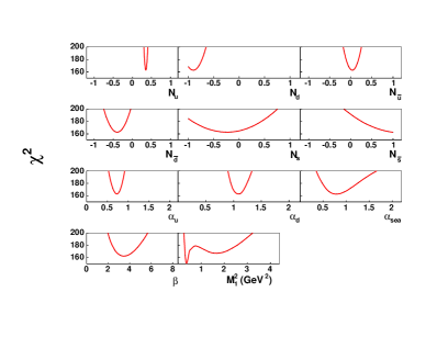
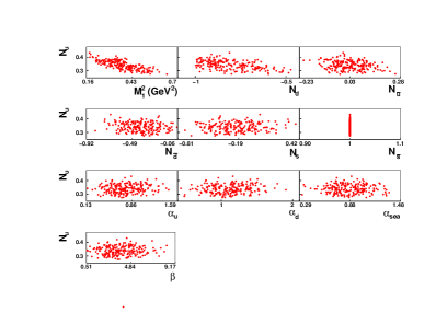
Figure 12: The shape of $\chi^{2}$ as a function of the fit parameters (left) and the scatter plot of the 200 generated sets as a function of $N_{u}$ (right).

References

- Anselmino et al. (2005a) M. Anselmino, et al., Phys. Rev. D71, 074006 (2005a), eprint arXiv:hep-ph/0501196.
- Anselmino et al. (2005b) M. Anselmino, et al., Phys. Rev. D72, 094007 (2005b), eprint arXiv:hep-ph/0507181.
- Airapetian et al. (2005) A. Airapetian, et al., Phys. Rev. Lett. 94, 012002 (2005), eprint arXiv:hep-ex/0408013.
- Alexakhin et al. (2005) V. Y. Alexakhin, et al., Phys. Rev. Lett. 94, 202002 (2005), eprint arXiv:hep-ex/0503002.
- Sivers (1990) D. W. Sivers, Phys. Rev. D41, 83 (1990).
- Sivers (1991) D. W. Sivers, Phys. Rev. D43, 261 (1991).
- Vogelsang and Yuan (2005) W. Vogelsang, and F. Yuan, Phys. Rev. D72, 054028 (2005), eprint arXiv:hep-ph/0507266.
- Collins et al. (2006) J. C. Collins, et al., Phys. Rev. D73, 014021 (2006), eprint arXiv:hep-ph/0509076.
- Anselmino et al. (????) M. Anselmino, et al., in Transversity 2005, World Scientific, Singapore (2006), p. 236, eprint arXiv:hep-ph/0511017.
- Diefenthaler (2007) M. Diefenthaler (HERMES), eprint arXiv:0706.2242 [hep-ex].
- Martin (2006) A. Martin (COMPASS), Czech. J. Phys. 56, F33 (2006), eprint arXiv:hep-ex/0702002.
- Alekseev et al. (2008) M. Alekseev, et al. (COMPASS), eprint arXiv:0802.2160 [hep-ex].
- de Florian et al. (2007) D. de Florian, R. Sassot, and M. Stratmann, Phys. Rev. D75, 114010 (2007), eprint arXiv:hep-ph/0703242.
- Mulders and Tangerman (1996) P. J. Mulders, and R. D. Tangerman, Nucl. Phys. B461, 197 (1996), eprint arXiv:hep-ph/9510301.
- Bacchetta et al. (2004) A. Bacchetta, U. D’Alesio, M. Diehl, and C. A. Miller, Phys. Rev. D70, 117504 (2004), eprint arXiv:hep-ph/0410050.
- Bacchetta et al. (2007) A. Bacchetta, et al., JHEP 02, 093 (2007), eprint arXiv:hep-ph/0611265.
- Anselmino et al. (2008) M. Anselmino, M. Boglione, U. D’Alesio, S. Melis, F. Murgia, and A. Prokudin, in preparation.
- Ji et al. (2005) X.-D. Ji, J.-P. Ma, and F. Yuan, Phys. Rev. D71, 034005 (2005), eprint arXiv:hep-ph/0404183.
- Ji et al. (2004) X.-D. Ji, J.-P. Ma, and F. Yuan, Phys. Lett. B597, 299 (2004), eprint arXiv:hep-ph/0405085.
- Ji et al. (2006) X.-D Ji, J.-W. Qiu, W. Vogelsang, and F. Yuan, Phys. Lett. B638, 1782 (2006), eprint arXiv:hep-ph/0604128.
- Kretzer (2000) S. Kretzer, Phys. Rev. D62, 054001 (2000), eprint arXiv:hep-ph/0003177.
- Hirai et al. (2007) M. Hirai, S. Kumano, T. H. Nagai, and K. Sudoh, Phys. Rev. D75, 094009 (2007), eprint arXiv:hep-ph/0702250.
- Prokudin et al. (Dubna, Russia, September 3-7, 2007) A. Prokudin, et al., Proceedings of the XII Workshop on High Energy Spin Physics, DSPIN-07, Dubna, Russia, September 3-7, 2007, URL http://theor.jinr.ru/~spin/Spin-Dubna07/2%204TuA/6%20Prokudin%/prokudin_dubna.pdf.
- Arnold et al. (2008) S. Arnold, A. V. Efremov, K. Goeke, M. Schlegel, and P. Schweitzer, eprint arXiv:0805.2137 [hep-ph].
- Gluck et al. (1998) M. Glück, E. Reya, and A. Vogt, Eur. Phys. J. C5, 461 (1998), eprint arXiv:hep-ph/9806404.
- Airapetian et al. (2008) A. Airapetian, et al. (HERMES), Phys. Lett. B666, 446 (2008), eprint arXiv:0803.2993 [hep-ex].
- Pumplin et al. (2002) J. Pumplin, et al., JHEP 07, 012 (2002), eprint arXiv:hep-ph/0201195.
- Martin et al. (2002) A. D. Martin, R. G. Roberts, W. J. Stirling, and R. S. Thorne, Phys. Lett. B531, 216 (2002), eprint arXiv:hep-ph/0201127.
- Pobylitsa (2003) P. V. Pobylitsa, eprint arXiv:hep-ph/0301236.
- Drago (2005) A. Drago, Phys. Rev. D71, 057501 (2005), eprint arXiv:hep-ph/0501282.
- Burkardt (2004) M. Burkardt, Phys. Rev. D69, 091501 (2004), eprint arXiv:hep-ph/0402014.
- Anselmino et al. (2006) M. Anselmino, U. D’Alesio, S. Melis, and F. Murgia, Phys. Rev. D74, 094011 (2006), eprint arXiv:hep-ph/0608211.
- Brodsky and Gardner (2006) S. J. Brodsky, and S. Gardner, Phys. Lett. B643, 22 (2006), eprint arXiv:hep-ph/0608219.
- Yao et al. (2006) W.-M. Yao, et al., Particle Data Group, J. Phys. G33, 301 (2006), URL http://pdg.lbl.gov.
- Press et al. (2007) W. H. Press, S. A. Teukolsky, W. T. Vetterling, and B. P. Flannery, Numerical Recipes, Cambridge University Press, Third Edition, p. 1256 (2007), URL http://www.nr.com.