Temperature and magnetic-field dependence of the quantum corrections to the conductance of a network of quantum dots

Abstract

We calculate the magnetic-field and temperature dependence of all quantum corrections to the ensemble-averaged conductance of a network of quantum dots. We consider the limit that the dimensionless conductance of the network is large, so that the quantum corrections are small in comparison to the leading, classical contribution to the conductance. For a quantum dot network the conductance and its quantum corrections can be expressed solely in terms of the conductances and form factors of the contacts and the capacitances of the quantum dots. In particular, we calculate the temperature dependence of the weak localization correction and show that it is described by an effective dephasing rate proportional to temperature.

I Introduction

The low temperature conductivity of disordered metals or semiconductors is dominated by the elastic scattering of electrons off impurities and defects. While the conductivity is determined by Drude-Boltzmann theory for not too low temperatures, quantum corrections to the conductivity become important at temperatures low enough that the electronic phase remains well defined over distances large in comparison to the elastic mean free path.Altshuler and Aronov (1985); Altshuler and Simons (1995); Imry (2002) One usually distinguishes two quantum corrections, the weak localization correction and the interaction correction.Anderson et al. (1979); Gorkov et al. (1979); Altshuler and Aronov (1979a) The former is caused by the constructive interference of electrons traveling along time-reversed paths, whereas the interaction correction can be understood in terms of resonant scattering off Friedel oscillations near impurities.Aleiner et al. (1999); Zala et al. (2001)

Although they are small in comparison to the Drude conductivity, the quantum corrections are important because they strongly depend on temperature and an applied magnetic field, whereas the Drude conductivity does not (as long as impurity scattering is the dominant source of scattering). Theoretically, the temperature and magnetic-field dependences of the corrections can be expressed in terms of the sample’s diffusion constant (or, equivalently, the elastic mean free path), which can be obtained independently from a measurement of the Drude conductivity. The availability of quantitative theoretical predictions has made a detailed comparison between theory and experiment possible.Bouchiat (1995); Pierre et al. (2003); endnote83

The same quantum corrections also exist for a ‘quantum dot’, a conductor coupled to electron reservoirs via artificial constrictions (e.g., tunnel barriers or point contacts), such that the conductance of the device is dominated by the contacts and not by scattering off impurities or defects inside the sample. The latter condition is satisfied if the product $E_{\rm Th}\nu$ of the dot’s ‘Thouless energy’ and its density of states is much larger than the dimensionless conductance of the contacts connecting the dot to source and drain reservoirs. (The Thouless energy is the inverse of the time needed for ergodic exploration of the quantum dot.)

In this article we consider ‘open’ quantum dots, which have contact conductances larger than the conductance quantum $e^{2}/h$. Because transport through a quantum dot is dominated by the contacts, it is described by the sample’s conductance, not its conductivity. The quantum corrections then pertain to the conductance after averaging over an ensemble of quantum dots that differ, e.g., in their shape or precise impurity configuration.

While the magnetic-field dependence of quantum corrections to the ensemble averaged conductance is in apparent agreement with the theory,Marcus et al. (1997) the situation regarding the temperature dependence is more complicated and no good agreement has been reported to date. Theoretically, the temperature dependence of the weak localization correction to the conductance of a quantum dot is described by means of a ‘dephasing rate’ $\gamma_{\phi}$. For a quantum dot, one expects

$$\gamma_{\phi}=cT^{2}/E_{\rm Th}^{2}\nu,$$ (1)

where $T$ is the temperature and $c$ is a numerical constant that depends on the dot’s size and shape.Sivan et al. (1994); Ya. M. Blanter (1996); endnote84 The proportionality constant $c$ can not be measured independently, however, which is an important difference with the case of a diffusive conductor. The absence of a separate method to determine this constant poses a significant difficulty when comparing theory and experiment. A second difficulty is the lack of a direct theory of the temperature dependence of weak localization. Instead, the available theoretical descriptions employ a phenomenological description Marcus et al. (1993); Clarke et al. (1995); Baranger and Mello (1995); Brouwer (1995); Beenakker and Michaelis (2005); Forster et al. (2007) and match the dephasing rate to Eq. (1), from which the temperature dependence of weak localization can be obtained.

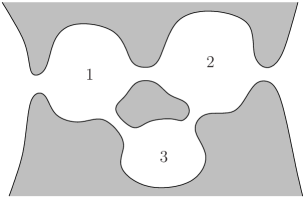
Figure 1: An example of a quantum dot network with $\mathcal{N}_{\rm D}=3$ quantum dots. The conductance of the network is dominated by the conductances of the contacts between the dots. We assume that all dots in the network are ‘open’, i.e., all contact conductances are much larger than the conductance quantum $e^{2}/h$.

In this article, we study the quantum corrections to the conductance in a network of quantum dots or “quantum circuit”.Nazarov (1994) (See Fig. 1 for an example of a quantum dot network with $\mathcal{N}_{\rm D}=3$ dots.) Replacing a single quantum dot by a network solves both difficulties mentioned above: A quantum dot network allows a calculation of the complete temperature dependence of the quantum corrections to the conductance without the need of an intermediate step involving a phenomenological dephasing rate and without parameters that can not be measured independently. The relevant parameters in a quantum dot network are the conductances and form factors of the contacts in the network and the capacitances of the quantum dots.endnote85

Our main result is an expression for the ensemble average of the dimensionless conductance

$$G=\frac{d_{\rm s}e^{2}}{h}g,$$ (2)

where $d_{\rm s}=$ 1 or 2 in the absence or presence of spin degeneracy, respectively. The result becomes exact in the limit that the contact conductances are much larger than the conductance quantum $e^{2}/h$,

$$\langle g\rangle=g^{\rm cl}+\delta g^{\rm WL}+\delta g^{{\rm int},1}+\delta g^{{\rm int},2}.$$ (3)

Here $g^{\rm cl}$ is the ‘classical’ conductance one obtains from Drude-Boltzmann theory, while $\delta g^{\rm WL}$, $\delta g^{{\rm int},1}$, and $\delta g^{{\rm int},2}$ are three quantum corrections to $\langle g\rangle$. Explicit expressions for $g^{\rm cl}$ and the three quantum corrections in terms of the contact conductances and the capacitances of the quantum dots in the network, as well as the precise conditions for the validity of Eq. (3) will be given in Sec. II below. The correction $\delta g^{\rm WL}$ is the weak localization correction. It is the only quantum correction that is affected by the application of a magnetic field. The remaining two corrections arise from electron-electron interactions. The first interaction correction $\delta g^{{\rm int},1}$ represents a non-local correction to the conductance that exists for networks of two or more quantum dots only.Beloborodov et al. (2003a); Golubev and Zaikin (2004a); Brouwer and Kupferschmidt (2007) It is the counterpart of the Altshuler-Aronov correction in the theory of disordered conductors. The second correction, $\delta g^{{\rm int},2}$, describes the renormalization of the contact conductances by the interactions. It is usually referred to as (dynamical) Coulomb blockade, an effect that is well-known from the theory of transport through tunnel junctions in series with a high impedance or quantum dots with tunneling contacts.Devoret et al. (1990); Girvin et al. (1990); Yu. V. Nazarov (1989); Flensberg (1993); Furusaki and Matveev (1995a, b); Golubev and Zaikin (2001); Levy Yeyati et al. (2001); Kindermann and Yu. V. Nazarov (2003); Golubev and Zaikin (2004b); Bagrets and Yu. V. Nazarov (2005); Brouwer et al. (2005a, b) Its counterpart in the theory of disordered conductors is the Altshuler-Aronov correction to the tunneling density of states.Altshuler and Aronov (1979b)

The fact that the temperature dependence of quantum corrections in a quantum dot network does not depend on details of individual dots has its origin in the different form of the relevant electron-electron interaction modes in a quantum dot network and in a single dot. In a single quantum dot, the dominant contribution to the electron-electron interaction is the uniform mode, the strength of which is set by the dot’s capacitance. Apart from a possible renormalization of the contact conductances, $\delta g^{{\rm int},2}$, the uniform mode has no effect on the quantum correction to the dot’s conductance.Golubev and Zaikin (2004b); Brouwer et al. (2005a, b); Ahmadian et al. (2005) In particular, the weak localization correction $\delta g^{\rm WL}$ is unaffected by the interaction and the non-local interaction correction $\delta g^{{\rm int},1}$ vanishes. Instead, electron-electron interactions determine $\delta g^{\rm WL}$ and $\delta g^{{\rm int},1}$ in a single quantum dot through sub-dominant non-uniform interaction modes, which are known to depend on the precise sample details.Sivan et al. (1994); Aleiner et al. (2002) For a quantum dot network, on the other hand, there exist interaction modes that are uniform inside each dot but not across the full network. With such interaction modes, all three interaction corrections $\delta g^{\rm WL}$, $\delta g^{\rm int,1}$, and $\delta g^{\rm int,2}$ are generically nonzero and temperature dependent. Moreover, because these modes are uniform inside each quantum dot, their properties depend on the contacts between the dots and on the dot capacitances only, not on the precise geometry of each dot separately. It is this essential feature that makes a quantum dot network an ideal paradigm for studying the effect of electron-electron interactions on quantum transport in finite-size systems.

Separate aspects of the problem we address here have been considered before. Weak localization in single quantum dots without interactions has been studied by various authors,Baranger and Mello (1994); Jalabert et al. (1994); Efetov (1995); Argaman (1995, 1996); Aleiner and Larkin (1996); Brouwer and Beenakker (1996); Vavilov and Aleiner (1999); Richter and Sieber (2002); Whitney (2007) as well as the effect of the uniform interaction mode on the conductances of the contacts connecting the dot to the electron reservoirs.Yu. V. Nazarov (1989); Girvin et al. (1990); Devoret et al. (1990); Flensberg (1993); Furusaki and Matveev (1995a, b); Golubev and Zaikin (2001); Levy Yeyati et al. (2001); Kindermann and Yu. V. Nazarov (2003); Golubev and Zaikin (2004b); Bagrets and Yu. V. Nazarov (2005); Brouwer et al. (2005a, b) (See Ref. Ahmadian et al., 2005 for a discussion of a comparable effect involving spin-dependent interactions in the quantum dot.) Also, while it is known that the uniform interaction mode has no effect on weak localization because a spatially uniform fluctuating potential affects phases of time-reversed trajectories in the same way,Brouwer et al. (2005a, b) the uniform interaction mode can suppress interference contributions to other observables if the quantum dot is part of an interferometer.Seelig and Büttiker (2001); Seelig et al. (2003); endnote86

Weak localization in networks of quantum dots, but without interactions, was considered by Argaman for dots connected by ideal contacts,Argaman (1995, 1996) and by Campagnano and Nazarov for dots connected by arbitrary contacts.Campagnano and Nazarov (2006) Golubev and Zaikin calculated the interaction corrections $\delta g^{{\rm int},1}$ and $\delta g^{{\rm int},2}$ for a linear array of quantum dots,Golubev and Zaikin (2004a) as well as the weak localization correction for non-interacting electrons (but with a phenomenological dephasing rate).Golubev and Zaikin (2006) In a recent publication, the same authors also considered the full temperature dependence of weak localization in the special case of a double quantum dot (a network with $\mathcal{N}_{\rm D}=2$ quantum dots) with tunneling contacts,Golubev and Zaikin (2007) and reported that electron-electron interactions suppress weak localization even at zero temperature, a conclusion that contradicts the common wisdom that there is no dephasing from electron-electron interactions at zero temperature.Altshuler and Aronov (1985); Imry (2002)

Weak localization and interaction corrections have also been considered for networks of diffusive metallic wires.Texier and Montambaux (2004, 2007) Large arrays of quantum dots connected by tunneling contacts further appear in the study of granular metals.Beloborodov et al. (2007) Beloborodov and coworkers considered the interaction corrections $\delta g^{{\rm int},1}$ and $\delta g^{{\rm int},2}$ for a granular metal,Beloborodov et al. (2001); Beloborodov et al. (2003b, a); Efetov and Tschersich (2003); Beloborodov et al. (2004) but accounted for weak localization and its temperature dependence only via a phenomenological dephasing rate and a renormalized diffusion constant. A microscopic theory of the temperature dependence of weak localization in granular metals was given by Blanter et al. in the high temperature limit.Blanter et al. (2006) Our present analysis (as well as that of Ref. Golubev and Zaikin, 2004a) is for contacts of arbitrary transparency and contains contributions to weak localization and to the interaction correction to the conductance that are absent in a network where all contacts are tunneling contacts. Our results agree with the literature wherever applicable, except for the zero-temperature limit of the weak localization correction $\delta g^{\rm WL}$, where we find that weak localization is unaffected by electron-electron interactions, in contrast to Ref. Golubev and Zaikin, 2007.

The remainder of our article is organized as follows. In Sec. II we introduce the relevant parameters needed to describe the quantum dot network, formulate our main assumptions, and present our main result, an expression for the ensemble-averaged conductance and its quantum corrections. In Sec. III we motivate our result for the temperature dependence of the weak localization correction using semiclassical arguments. In Sec. IV we then turn to a fully quantum mechanical calculation of the conductance and its quantum corrections using random matrix theory. We specialize to the simplest network, a double quantum dot, in Sec. V and discuss the origin of the difference between our result and Ref. Golubev and Zaikin, 2007 for the zero-temperature limit of weak localization. We conclude in Sec. VI.

II Definition of the problem and main results

II.1 Network of quantum dots

We consider a network of $\mathcal{N}_{\rm D}$ quantum dots, coupled to two electron reservoirs. A schematic drawing of a network is shown in Fig. 1. In this section we introduce the relevant parameters to describe the quantum dot network and summarize our main results.

The quantum dots are connected to each other and to source and drain electron reservoirs via point contacts. The dots will be labeled by an index $i=1,\ldots,\mathcal{N}_{\rm D}$; the reservoirs are labeled by the index $a=1,2$. The contact between dots $i$ and $j$ is described by its dimensionless conductance $g_{ij}$ (per spin direction) and its form factor $f_{ij}$. Both $g_{ij}$ and $f_{ij}$ are defined in terms of the transmission matrix $t_{ij}$ of the contact,

$$g_{ij} = \mbox{tr}\,t_{ij}t_{ij}^{\dagger},\ \ f_{ij}=\mbox{tr}\,(t_{ij}t_{ij}^{\dagger})^{2}.$$ (4)

Form factors are related to Fano factors $\beta$ often encountered in the literature via $\beta_{ij}=(g_{ij}-f_{ij})/g_{ij}$. The dimensionless conductances and form factors are symmetric, $g_{ij}=g_{ji}$ and $f_{ij}=f_{ji}$, $i,j=1,\ldots,\mathcal{N}_{\rm D}$. Spin degeneracy will be explicitly taken into account via the parameter $d_{\rm s}={1,2}$.

Similarly, the contacts between the $i$th quantum dot and reservoir $a$, $a=1,2$, are described by a dimensionless conductance $g_{ia}^{\prime}=g_{ai}^{\prime}$ and a form factor $f_{ia}^{\prime}=f_{ai}^{\prime}$, which are related to the transmission matrix $t_{ia}^{\prime}$ of these contacts as

$$g_{ia}^{\prime} = \mbox{tr}\,t_{ia}^{\prime}t_{ia}^{\prime\dagger},\ \ f_{ia}^{\prime}=\mbox{tr}\,(t_{ia}^{\prime}t_{ia}^{\prime\dagger})^{2}.$$ (5)

For ballistic contacts one has $f=g$; for tunneling contacts one has $f\ll g$. Throughout we assume that all conductances are large,

$$g_{ij},\ g_{ia}^{\prime},\gg 1,\ \ i,j=1,\ldots,\mathcal{N}_{\rm D},\ \ a=1,2.$$ (6)

(One may replace this condition by the less strict requirement that each quantum dot be well connected to one of the two reservoirs, such that the regime of strong Coulomb blockade is avoided.) For future use, we arrange the conductances and form factors in $\mathcal{N}_{\rm D}\times\mathcal{N}_{\rm D}$ matrices $\tilde{g}$ and $\tilde{f}$ with elements

$$\tilde{g}_{ij} = \left\{\begin{array}[]{ll}\sum_{a=1}^{2}g_{aj}^{\prime}+\sum_{k\neq i}^{\mathcal{N}_{\rm D}}g_{ik}&i=j,\\ -g_{ij}&i\neq j\mbox{,}\end{array}\right.$$ (9)

$$\tilde{f}_{ij} = \left\{\begin{array}[]{ll}\sum_{a=1}^{2}f_{aj}^{\prime}+\sum_{k\neq i}^{\mathcal{N}_{\rm D}}f_{ik}&i=j,\\ -f_{ij}&i\neq j\mbox{.}\end{array}\right.$$ (12)

The quantum dots are assumed to be disordered or ballistic-chaotic, with density of states $\nu_{i}$ per spin degree of freedom and Thouless energy $E_{{\rm Th},i}$, $i=1,\ldots,\mathcal{N}_{\rm D}$. The Thouless energy $E_{{\rm Th},i}=\hbar/\tau_{{\rm erg},i}$, where $\tau_{{\rm erg},i}$ is the time for ergodic exploration of the $i$th quantum dot. If the electron motion is diffusive inside each quantum dot with diffusion constant $D$, $E_{{\rm Th},i}\sim D/L_{i}^{2}$ where $L_{i}$ is the linear size of dot $i$. (Our definition, while common in the literature, differs from some references where $E_{{\rm Th},i}$ is the inverse of the dot’s dwell time.) We assume

$$E_{{\rm Th},i}\nu_{i}\gg\tilde{g}_{ii},\ \ i=1,\ldots,\mathcal{N}_{\rm D},$$ (13)

so that random matrix theory can be used to describe the electronic states in the quantum dot network. An external magnetic field is described by means of the dimensionless numbers

$$g_{{\rm H},i}=E_{{\rm Th},i}\nu_{i}\frac{\Phi_{i}^{2}}{\Phi_{0}^{2}},\ \ i=1,\ldots,\mathcal{N}_{\rm D},$$ (14)

where $\Phi_{i}$ is the magnetic flux through the $i$th quantum dot and $\Phi_{0}=hc/e$ is the flux quantum. In order to simplify the notation, we arrange the densities of states $\nu_{i}$ and the parameters $g_{{\rm H},i}$ in diagonal $\mathcal{N}_{\rm D}$-dimensional matrices $\tilde{\nu}$ and $\tilde{g}_{\rm H}$,

$$\tilde{\nu}_{ij}=\nu_{i}\delta_{ij},\ \ (\tilde{g}_{\rm H})_{ij}=g_{{\rm H},i}\delta_{ij},\ \ i,j=1,\ldots,\mathcal{N}_{\rm D}.$$ (15)

Corrections to the conductance that depend on the magnetic field will only be relevant where $g_{{\rm H},i}$ is of order $\tilde{g}_{ii}$ or less, otherwise they will be fully suppressed. In that parameter range, the flux through the insulating regions between the quantum dots is much smaller than $\Phi_{0}$, so that the corresponding Aharonov-Bohm phases can be neglected.

The inequality (13) also implies that the electron-electron interaction in each dot is well screened.Aleiner et al. (2002) Hence, the electron-electron interaction couples to the total charge $q_{i}=en_{i}$ of each dot only. Such an interaction is described by means of capacitances $C_{ij}$ for the capacitive coupling between dots (if $i\neq j$) and for each dot’s self-capacitance (if $i=j$). Again, we arrange the capacitances into an $\mathcal{N}_{\rm D}$-dimensional matrix $\tilde{C}$,

$$\tilde{C}_{ij} = \left\{\begin{array}[]{ll}\sum_{k=1}^{\mathcal{N}_{\rm D}}C_{ik}&i=j,\\ -C_{ij}&i\neq j.\end{array}\right.$$ (18)

For metallic dots, one has the inequality

$$\tilde{C}_{ii}/e^{2}\ll\nu_{i},\ \ i=1,\ldots,\mathcal{N}_{\rm D}.$$ (19)

II.2 Quantum corrections to the conductance

Our main result is a calculation of the ensemble-averaged conductance $\langle G\rangle=(d_{\rm s}e^{2}/h)\langle g\rangle$ of the quantum dot network as a function of temperature,

$$\langle g\rangle=g^{\rm cl}+\delta g^{\rm WL}+\delta g^{{\rm int},1}+\delta g^{{\rm int},2},$$

where $g^{\rm cl}$ is the classical conductance of the network and $\delta g^{\rm WL}$, $\delta g^{{\rm int},1}$, and $\delta g^{{\rm int},2}$ are corrections. The average conductance is calculated using the following limiting procedure for the parameters of the network:

1. We first take the limit (13) needed for the applicability of random matrix theory, while keeping the ratios $\nu_{i}/\nu_{j}$ and $T/\nu_{i}$, as well as the $g_{{\rm H},i}$ fixed, $i,j=1,\ldots,\mathcal{N}_{\rm D}$.

2. We then take the limit (6) of large contact conductances, while keeping the ratios $g_{ij}/g_{ik}$, $g_{ij}/g_{{\rm H},i}$, and $g_{ij}/g_{ia}^{\prime}$ fixed, $i,j,k=1,\ldots,\mathcal{N}_{\rm D}$, $a=1,2$.

3. Finally, we simplify our results using the inequality (19), if possible.

In all three limiting steps, the number $\mathcal{N}_{\rm D}$ of dots in the network is kept constant. Keeping the ratio $T/\nu_{i}$ fixed in the first limiting step eliminates interaction corrections from non-uniform interaction modes inside the quantum dots, see Eq. (1) above. In the second limiting step, we do not make any assumptions about the temperature, thus allowing for the full range of temperature-dependent effects that can be described within random matrix theory. We note that, while the classical conductance $g^{\rm cl}$ diverges in this limiting procedure, this divergence does not affect the temperature or magnetic-field dependence of $\langle g\rangle$ because $g^{\rm cl}$ does not depend on temperature or magnetic field. Corrections not included in Eq. (3) are either small in the limit (6) of large contact conductances or small in the limit (13) used to justify the use of random matrix theory.

The leading term $g^{\rm cl}$ in Eq. (3) reads

$$g^{\rm cl} = \sum_{i,j=1}^{\mathcal{N}_{\rm D}}g_{1i}^{\prime}(\tilde{g}^{-1})_{ij}g_{j2}^{\prime}$$ (20)

$$= g_{1\cdot}^{\prime}\tilde{g}^{-1}_{\cdot\cdot}g_{\cdot 2}^{\prime},$$

where, in the second line of Eq. (20), we have written “$\cdot$” to denote indices in adjacent factors that are summed over as in matrix multiplication. [Compare with the first line of Eq. (20).] This shorthand notation will be employed throughout the text.

The correction $\delta g^{\rm WL}$ is the weak localization correction to the ensemble-averaged conductance. It can be distinguished from the remaining two corrections $\delta g^{{\rm int},1}$ and $\delta g^{{\rm int},2}$ because $\delta g^{\rm WL}$ depends on an applied magnetic field whereas $\delta g^{\rm int}_{1}$ and $\delta g^{{\rm int},2}$ do not. We find

$$\delta g^{\rm WL} = 2\sum_{i,j=1}^{\mathcal{N}_{\rm D}}\,\tilde{c}_{ij}\,g_{1\cdot}^{\prime}(\tilde{g}_{\cdot i}^{-1}-\tilde{g}_{\cdot j}^{-1})(\tilde{g}-\tilde{f})_{ij}\tilde{g}_{j\cdot}^{-1}g_{\cdot 2}^{\prime}$$ (21)

$$\mbox{}+\sum_{i=1}^{\mathcal{N}_{\rm D}}\,\tilde{c}_{ii}\,(g_{1\cdot}^{\prime}\tilde{g}_{\cdot\cdot}^{-1}\tilde{f}_{\cdot i}-f_{1i}^{\prime})\tilde{g}_{i\cdot}^{-1}g_{\cdot 2}^{\prime}$$

$$\mbox{}+\sum_{i=1}^{\mathcal{N}_{\rm D}}\,\tilde{c}_{ii}\,g_{1\cdot}^{\prime}\tilde{g}_{\cdot i}^{-1}(\tilde{f}_{i\cdot}\tilde{g}^{-1}_{\cdot\cdot}g_{\cdot 2}^{\prime}-f_{i2}^{\prime})$$

$$\mbox{}-\sum_{i,j=1}^{\mathcal{N}_{\rm D}}\tilde{f}_{ij}\,\tilde{c}_{jj}\,g_{1\cdot}^{\prime}\tilde{g}_{\cdot i}^{-1}\tilde{g}_{i\cdot}^{-1}g_{\cdot 2}^{\prime},$$

where the $\mathcal{N}_{\rm D}\times\mathcal{N}_{\rm D}$ matrix $\tilde{c}$ is the counterpart of the “Cooperon” in the theory of weak localization in disordered conductors. For the quantum dot network, $\tilde{c}$ reads

$$\tilde{c}_{ij}=\sum_{k=1}^{\mathcal{N}_{\rm D}}\frac{1}{\pi\hbar\nu_{k}}(\Gamma+\Gamma_{\rm H}+\Gamma_{\phi})^{-1}_{ik,jk},$$ (22)

where $\Gamma$, $\Gamma_{\rm H}$, and $\Gamma_{\phi}$ are rank-four tensors,

$$\Gamma_{ik,jl} = \frac{1}{2\pi\hbar\nu_{i}}\tilde{g}_{ik}\delta_{jl}+\frac{1}{2\pi\hbar\nu_{j}}\delta_{ik}\tilde{g}_{jl}$$

$$(\Gamma_{\rm H})_{ik,jl} = \frac{1}{2\pi\hbar\nu_{i}}\tilde{g}_{{\rm H},ik}\delta_{jl}+\frac{1}{2\pi\hbar\nu_{j}}\delta_{ik}\tilde{g}_{{\rm H},jl},$$

$$(\Gamma_{\phi})_{ik,jl} = \frac{4\pi T}{d_{\rm s}\hbar}(\tilde{g}^{-1}_{ii}+\tilde{g}^{-1}_{jj}-2\tilde{g}^{-1}_{ij})\delta_{ik}\delta_{jl}.$$ (23)

The terms $\Gamma_{\rm H}$ and $\Gamma_{\phi}$ describe the suppression of weak localization by a magnetic field and electron-electron interactions, respectively. In the limit of low temperatures $\Gamma_{\phi}=0$ and Eq. (22) simplifies to

$$\tilde{c}_{ij}=(\tilde{g}+\tilde{g}_{\rm H})^{-1}_{ij}.$$ (24)

For high temperatures $(\Gamma_{\phi})_{ii,jj}$ diverges [other elements are zero because of the Kronecker deltas in Eq. (II.2)], except for the diagonal elements with $i=j$. Hence, one finds

$$\tilde{c}_{ij}\equiv\tilde{c}_{ij}^{\rm d}=(\tilde{g}^{\rm d}+\tilde{g}_{\rm H})^{-1}_{ij},$$ (25)

where $\tilde{g}^{\rm d}_{ij}$ is the diagonal part of the matrix $\tilde{g}$, $\tilde{g}^{\rm d}_{ij}=\tilde{g}_{ij}\delta_{ij}$. This is the contribution to the weak localization correction that arises from self-returning electron trajectories that reside inside one quantum dot only and, hence, are unaffected by dephasing from electron-electron interactions.Blanter et al. (2006)

The first interaction correction $\delta g^{{\rm int},1}$ is

$$\delta g^{{\rm int},1} = \frac{2\pi}{d_{\rm s}}\int d\omega\left(\frac{\partial}{\partial\omega}\omega\coth\frac{\omega}{2T}\right)\sum_{\alpha,\beta=1}^{\mathcal{N}_{\rm D}}\sum_{k,l=1}^{\mathcal{N}_{\rm D}}\mbox{Im}\,\Big{[}\nu_{\alpha}(2\pi i\omega\tilde{g}^{-1}_{\alpha\beta}-\tilde{\nu}^{-1}_{\alpha\beta})\nu_{\beta}$$ (26)

$$\mbox{}\times(\tilde{g}-2\pi i\tilde{\nu}\omega)^{-1}_{\alpha k}(\tilde{g}-2\pi i\tilde{\nu}\omega)_{kl}(\tilde{g}-2\pi i\tilde{\nu}\omega)^{-1}_{\beta l}g_{1\cdot}(\tilde{g}^{-1}_{\cdot\alpha}-\tilde{g}^{-1}_{\cdot k})(\tilde{g}^{-1}_{l\cdot}-\tilde{g}^{-1}_{\beta\cdot})g_{\cdot 2}^{\prime}\Big{]}.$$

The second interaction correction $\delta g^{{\rm int},2}$ represents the renormalization of the conductances between the quantum dots and between the dots and the reservoirs as a result of the electron-electron interactions,

$$\delta g^{{\rm int},2} = \sum_{j=1}^{\mathcal{N}_{\rm D}}\sum_{a=1}^{2}\frac{\partial g_{\rm cl}}{\partial g_{aj}^{\prime}}\delta g_{aj}^{\prime}+\sum_{j<k}^{\mathcal{N}_{\rm D}}\frac{\partial g_{\rm cl}}{\partial g_{jk}}\delta g_{jk}.$$ (27)

The interaction corrections $\delta g_{ia}^{\prime}$ and $\delta g_{ij}$ exist for non-ideal contacts with $f_{ij}<g_{ij}$, $f_{ia}^{\prime}<g_{ia}^{\prime}$ only, $i,j=1,\ldots,\mathcal{N}_{\rm D}$, $a=1,2$,

$$\delta g_{aj}^{\prime} = -(g_{aj}^{\prime}-f^{\prime}_{aj})\int\frac{d\omega}{\omega}\left(\frac{\partial}{\partial\omega}\omega\coth\frac{\omega}{2T}\right)\mbox{Re}\,\delta\tilde{z}_{jj},$$

$$\delta g_{jk} = -(g_{jk}-f_{jk})\int\frac{d\omega}{\omega}\left(\frac{\partial}{\partial\omega}\omega\coth\frac{\omega}{2T}\right)$$ (28)

$$\mbox{}\times\mbox{Re}\,(\delta\tilde{z}_{jj}+\delta\tilde{z}_{kk}-2\delta\tilde{z}_{jk}),$$

where $\delta\tilde{z}$ is the difference of the network’s dimensionless impedance matrices with and without interactions,

$$\delta\tilde{z}=(d_{\rm s}\tilde{g}-2\pi i\omega\tilde{C}/e^{2})^{-1}-(d_{\rm s}\tilde{g}-2\pi i\omega d_{\rm s}\tilde{\nu})^{-1}.$$ (29)

The interaction correction $\delta g^{{\rm int},1}$ was obtained previously by Golubev and Zaikin for a linear array of quantum dots,Golubev and Zaikin (2004a) and by Beloborodov et al. in the context of a granular metal.Beloborodov et al. (2003a) It is the counterpart of the Altshuler-Aronov correction in disordered metals, where it arises from the diffusive dynamics of the electrons. Although the electron dynamics is not diffusive in a quantum dot network, it is non-ergodic, which is sufficient for this interaction correction to appear. (The exception is a quantum dot network consisting of a single quantum dot only, for which the electron motion is ergodic. Indeed, one verifies that $\delta g^{{\rm int},1}=0$ if $\mathcal{N}_{\rm D}=1$, in agreement with Refs. Golubev and Zaikin, 2004b, a; Brouwer et al., 2005a, b.) A semiclassical calculation of $\delta g^{{\rm int},1}$ for the special case of a double quantum dot with ballistic contacts can be found in Ref. Brouwer and Kupferschmidt, 2007.

For the case of a single quantum dot, the renormalization of the contact conductances $\delta g^{{\rm int},2}$ or “dynamical Coulomb blockade” was obtained previously in Refs. Golubev and Zaikin, 2001; Levy Yeyati et al., 2001; Kindermann and Yu. V. Nazarov, 2003; Golubev and Zaikin, 2004b; Bagrets and Yu. V. Nazarov, 2005; Brouwer et al., 2005a, b. The renormalization of the contact conductances in the quantum dot network is essentially the same as in the case of a single quantum dot or a single tunnel junction coupled to a high-impedance electrical environment — in both cases the change of the contact conductance is proportional to the factor $(g-f)$ —, the only difference being that the impedance $z$ is replaced by the impedance matrix $\tilde{z}$ in the case of the quantum dot network.Golubev and Zaikin (2004a) The same conclusion was reached for the interaction correction in an array of quantum dots with tunneling contacts in the context of transport through a granular metal.Beloborodov et al. (2001); Beloborodov et al. (2003b, a); Efetov and Tschersich (2003); Beloborodov et al. (2004)

Equations (3)–(29) provide a general solution for the ensemble-averaged conductance and its quantum corrections in an arbitrary quantum dot network for arbitrary temperature. These expressions can be simplified only by specializing to a particular quantum dot network. In Sec. V we analyze these expressions for the case of a double quantum dot, a network consisting of two quantum dots.

Although it is not possible to proceed quantitatively without specializing to a particular network, we can compare the sizes of these three quantum corrections and their typical temperature dependences. For the limiting procedure taken here — see the discussion following Eq. (3) —, the relevant temperature scale for dephasing of the weak localization correction isBlanter et al. (2006)

$$T_{\phi}=\hbar\max(g,g_{\rm H})/\tau_{\rm D},$$ (30)

where

$$\tau_{\rm D}\sim\hbar\nu/g$$ (31)

is the typical dwell time for the network. (Here $g$ and $g_{\rm H}$ are shorthand notations for typical values of $g_{ij}$ or $g_{{\rm H},i}$ in the network, respectively.) For the interaction corrections $\delta g^{{\rm int},1}$ and $\delta g^{{\rm int},2}$, the relevant temperature scales are $\hbar/\tau_{\rm D}$ and the inverse charge relaxation time

$$\hbar/\tau_{\rm c}\sim e^{2}g/\hbar C.$$ (32)

(In a more precise analysis one needs to identify $\mathcal{N}_{\rm D}$ dwell times and $\mathcal{N}_{\rm D}$ charge relaxation times for a network consisting of $\mathcal{N}_{\rm D}$ quantum dots, see Sec. V for an explicit calculation for $\mathcal{N}_{\rm D}=2$.) Since, typically, $C/e^{2}\ll\nu$, the charge relaxation time and the dwell time satisfy the inequality

$$\tau_{\rm c}\ll\tau_{\rm D}.$$ (33)

With these definitions, we find the order of magnitude of the weak localization correction $\delta g^{\rm WL}$ to be

$$\delta g^{\rm WL}\sim\delta g_{\rm WL}^{\rm d}+\frac{\delta g_{\rm WL}^{\rm od}}{\max(1,T/T_{\phi})},$$ (34)

where $\delta g_{\rm WL}^{\rm d}$ and $\delta g_{\rm WL}^{\rm od}$ are constants of order $\min(1,g/g_{\rm H})$. Similarly, for interaction corrections we find

$$\delta g^{{\rm int},1} \sim \min(1,\hbar/T\tau_{\rm D}),$$ (35)

$$\delta g^{{\rm int},2} \sim \left\{\begin{array}[]{ll}\ln[\max(\tau_{\rm c}T/\hbar,\tau_{\rm c}/\tau_{\rm D})]&\mbox{if $T\ll\hbar/\tau_{\rm c}$},\\ \hbar/T\tau_{\rm c}&\mbox{if $T\gg\hbar/\tau_{\rm c}$},\end{array}\right.~{}~{}~{}~{}$$ (38)

independent of the magnetic field. All three quantum corrections need to be taken into account for a complete description of the temperature and magnetic-field dependence of the conductance of a quantum dot network. In particular, in order to correctly describe the temperature dependence of $\langle g\rangle$ for $T\lesssim\hbar/\tau_{\rm D}$, $\delta g^{{\rm int},1}$ can not be neglected with respect to $\delta g^{{\rm int},2}$, in spite of the fact that $\delta g^{{\rm int},2}$ is larger than $\delta g^{{\rm int},1}$ by (at least) a large logarithmic factor $\ln(\tau_{\rm D}/\tau_{\rm c})$.

The temperature dependence (34) implies a dephasing rate that is linear in temperature. A linear temperature dependence of the dephasing rate was obtained previously by Blanter et al. in the context of a granular metal,Blanter et al. (2006) and by Seelig and Büttiker for a single quantum dot embedded in one arm of an interferometer.Seelig and Büttiker (2001) In both cases, the linear temperature dependence of the dephasing rate arose because the fluctuations of the electric potential can be considered classical, similar to the situation encountered in one-dimensional and two-dimensional disordered conductors.Altshuler et al. (1982) As we discuss in the following sections, the same mechanism is responsible for the linear temperature dependence of the dephasing rate in the quantum dot network.

In the next section we describe a semiclassical derivation of the weak localization correction and its temperature dependence, Eq. (21) above. A full quantum mechanical calculation of all three corrections to the conductance is given in Sec. IV. We apply the general results presented here to the specific case of a double quantum dot in Sec. V.

III Weak localization: semiclassical considerations

In this section, we give a semiclassical argument for the temperature dependence of the weak localization correction to the conductance of a quantum dot network. These arguments provide a semiclassical interpretation of the fully quantum mechanical calculations of the next section.

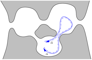
Figure 2: Schematic drawing of a trajectory $\alpha$ and its time-reversed $\bar{\alpha}$ that contribute to the Cooperon propagator $\tilde{c}$.

Weak localization appears because of constructive interference of time-reversed trajectories. This interference leads to a small increase to the probability $P_{\rm ret}$ that an electron returns to its point of origin. Following the standard arguments,Imry (2002); Altshuler and Simons (1995) $P_{\rm ret}$ is calculated as a square of the return amplitude which, in turn, is written as a sum of amplitudes $A_{\alpha}$ over all returning paths $\alpha$. (These paths are classical paths in ballistic conductors,Aleiner and Larkin (1996); Richter and Sieber (2002) and quantum diffractive paths in conductors with impurity scattering.) The quantum correction to $P_{\rm ret}$ then follows from interference between a path $\alpha$ and its time-reversed $\bar{\alpha}$. Since the length of the self-returning path is arbitrary, the weak localization correction to the dc conductance is proportional to the time integral of the interference correction to the return probability, known as the “Cooperon” in the diagrammatic theory of weak localization.Imry (2002); Altshuler and Simons (1995) The counterpart of the Cooperon for the quantum dot network is the quantity

$$\tilde{c}_{ij}\sim\frac{1}{(2\pi\hbar)^{2}\nu_{i}\nu_{j}}\sum_{\alpha}A_{\alpha}(A_{\bar{\alpha}})^{*},$$ (39)

where the sum is over all trajectories $\alpha$ that originate in dot $j$ and end in dot $i$ and $\bar{\alpha}$ is the time-reversed of $\alpha$, see Fig. 2. [Note that the return probability involves the diagonal elements $\tilde{c}_{ii}$ of the Cooperon matrix only. We have included non-diagonal elements in Eq. (39) above in view of the discussion of interaction effects below. Non-diagonal elements $\tilde{c}_{ij}$ with $i$ and $j$ in adjacent dots also appear for the description of weak localization in a network of quantum dots with tunneling contacts, see Eq. (21) above.]

At zero temperature and without a magnetic field, $A_{\bar{\alpha}}=A_{\alpha}$. We may then calculate $\tilde{c}_{ij}$ using that $|A_{\alpha}|^{2}$ is the probability that an electron propagates along trajectory $\alpha$. Hence

$$\tilde{c}_{ij} = \frac{1}{2\pi\hbar\nu_{i}}\int_{0}^{\infty}d\tau P_{ij}(\tau),$$ (40)

where $P_{ij}(\tau)$ is the probability that an electron in dot $j$ is found in dot $i$ after time $\tau$. In Eq. (40) we canceled a factor $2\pi\hbar\nu_{j}$ in the denominator against the phase space volume of the $j$th quantum dot. For a quantum dot network, $P_{ij}(\tau)$ can be expressed in terms of a rate matrix $\tilde{\gamma}$,

$$P_{ij}(\tau)=(e^{-\tilde{\gamma}\tau})_{ij},\ \ \tilde{\gamma}=\tilde{g}/(2\pi\hbar\tilde{\nu}).$$ (41)

Integrating over time, we then find

$$\tilde{c}_{ij}=\tilde{g}^{-1}_{ij}.$$ (42)

The interference between a path $\alpha$ and its time-reversed is suppressed if time-reversal symmetry is broken by a magnetic field, because a magnetic field changes the phases of $A_{\alpha}$ and $A_{\bar{\alpha}}$ in opposite ways. Interference is also suppressed because of electron-electron interactions at a finite temperature. Interactions cause the electrons to experience a time-dependent potential $\phi(\vec{r},t)$, which modifies the phase of $A_{\alpha}$ and $A_{\bar{\alpha}}$ in different ways if the trajectories $\alpha$ and $\bar{\alpha}$ are in different dots at the same time $t$.Altshuler et al. (1982) For a network of quantum dots, the fluctuating potential $\phi$ is uniform inside each dot, so that we can write $\phi(j,t)$, where $j=1,\ldots,\mathcal{N}_{\rm D}$ is the index labeling the quantum dots in the network. For each amplitude $A_{\alpha}$ one then hasAltshuler et al. (1982)

$$A_{\alpha}[\phi]\to A_{\alpha}[0]e^{i\int_{0}^{t_{\alpha}}\phi(j_{\alpha}(t),t)/\hbar},$$ (43)

where $t_{\alpha}$ is the duration of the path $\alpha$, $j_{\alpha}(t)$ the index of the quantum dot corresponding to the position of path $\alpha$ at time $t$, and $A_{\alpha}[0]$ the return amplitude in the absence of the potential $\phi$.

For a quantum dot network, one may consider $\phi$ as a classical fluctuating potential. (This will be verified in the exact quantum mechanical calculation of Sec. IV.2 below.) Its fluctuations are given by the fluctuation-dissipation relation,Landau and Lifshitz (1958)

$$\langle\phi(i,t)\phi(j,t^{\prime})\rangle = \int\frac{d\omega}{2\pi}e^{-i\omega(t-t^{\prime})/\hbar}\frac{2T}{\omega}\mbox{Im}\left[L^{\rm R}_{ij}(\omega)\right],$$

where the response function $L^{\rm R}_{ij}(\omega)$ describes the (linear) change $\delta\phi_{i}/e$ of the electric potential in the $i$th quantum dot to a change $\delta q_{j}=e\delta n_{j}$ of the charge in the $j$th quantum dot,

$$\delta\phi_{i}(\omega)=-L_{ij}^{\rm R}(\omega)\delta n_{j}(\omega).\ \$$ (45)

For the quantum dot network, one has

$$L_{ij}^{\rm R}(\omega)=-\left[\tilde{C}/e^{2}+d_{\rm s}(\tilde{\nu}^{-1}-2\pi i\omega\tilde{g}^{-1})^{-1}\right]^{-1}_{ij},$$ (46)

where the matrices $\tilde{C}$, $\tilde{\nu}$, and $\tilde{g}$ were defined in Sec. II above. Typically, $\tilde{C}_{ii}/e^{2}\ll\nu_{i}$, $\tilde{g}_{ii}/|\omega|$, and we can replace Eq. (46) by

$$L_{ij}^{\rm R}(\omega)=\frac{1}{d_{\rm s}}(2\pi i\omega\tilde{g}^{-1}-\tilde{\nu}^{-1})_{ij}.\ \$$ (47)

Using this expression for $L^{\rm R}_{ij}(\omega)$, we find that Eq. (III) simplifies to

$$\langle\phi(i,t)\phi(j,t^{\prime})\rangle = \frac{4\pi\hbar T}{d_{\rm s}}\,\tilde{g}^{-1}_{ij}\,\delta(t-t^{\prime}).$$ (48)

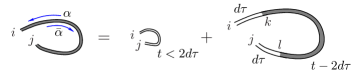
Figure 3: Calculation of the Cooperon propagator for a network of quantum dots. A trajectory $\alpha$ originating in dot $j$ and ending in dot $i$ and duration $t$ is separated into two segments of duration $d\tau$ and a remaining segment of duration $t-2d\tau$ if $2d\tau<t$. A self-consistent equation for $\tilde{c}_{ij}$ is obtained by considering the combined effect of escape, the magnetic field, and the fluctuating potential to first order in $d\tau$.

In order to find the effect of the fluctuating potential on the Cooperon propagator $\tilde{c}_{ij}$, we separate the contributions from trajectories $\alpha$ of duration $t_{\alpha}$ smaller and larger than $2d\tau$, where $d\tau$ is a time interval sufficiently short that the net phase shift from the fluctuating potential in the exponent in Eq. (43) is small, see Fig. 3. We also take $d\tau$ much shorter than the dwell time in a single quantum dot, so that $P_{ij}(d\tau)=\delta_{ij}-\tilde{\gamma}_{ij}d\tau$, see Eq. (41) above. For trajectories of duration $t_{\alpha}>2d\tau$ we consider the initial and final segment of duration $d\tau$ separately. Recognizing that the contribution from the intermediate segments of duration $t_{\alpha}-2d\tau$ can again be expressed in terms of $\tilde{c}$, and using Eq. (48) to average over the fluctuating potentials, we then find

$$\tilde{c}_{ij} = \frac{2d\tau}{2\pi\hbar\nu_{i}}\delta_{ij}$$ (49)

$$\mbox{}+\sum_{k,l=1}^{\mathcal{N}_{\rm D}}(\delta_{ik}-\tilde{\gamma}_{ki}d\tau)(\delta_{jl}-\tilde{\gamma}_{lj}d\tau)\tilde{c}_{kl}$$

$$\mbox{}-\sum_{k,l=1}^{\mathcal{N}_{\rm D}}(\tilde{\gamma}_{{\rm H},ik}+\tilde{\gamma}_{{\rm H},jl}+\tilde{\gamma}_{\phi,ij})\delta_{ik}\delta_{jl}\tilde{c}_{kl}d\tau,$$

$$= \tilde{c}_{ij}+\frac{d\tau}{\pi\hbar\nu_{i}}\delta_{ij}-(\Gamma+\Gamma_{\rm H}+\Gamma_{\phi})_{ik,jl}\tilde{c}_{kl}d\tau,$$

up to corrections of order $d\tau^{2}$. Here

$$\tilde{\gamma}_{{\rm H},ij} = \frac{g_{{\rm H},i}}{2\pi\hbar\nu_{i}}\delta_{ij},$$

$$\tilde{\gamma}_{\phi,ij} = \frac{4\pi T}{d_{\rm s}\hbar}(\tilde{g}^{-1}_{ii}+\tilde{g}^{-1}_{jj}-2\tilde{g}^{-1}_{ij}),$$ (50)

and $\Gamma_{ik,jl}=\tilde{\gamma}_{ki}\delta_{jl}+\delta_{ik}\tilde{\gamma}_{lj}$, $(\Gamma_{\rm H})_{ik,jl}=\tilde{\gamma}_{{\rm H},ik}\delta_{jl}+\delta_{ik}\tilde{\gamma}_{{\rm H},jl}$, $(\Gamma_{\phi})_{ik,jl}=\tilde{\gamma}_{\phi,ij}\delta_{ik}\delta_{jl}$, cf. Eq. (II.2) above. Solving this equation for $\tilde{c}$, we arrive at Eq. (22) of the previous section.

It is worth while to point out that the temperature dependence of weak localization is caused by processes that involve the exchange of energy quanta small in comparison to the temperature. Such processes are commonly referred to as “dephasing”, in contrast to more general inelastic processes which lead to a broadening of the electronic distribution function.Altshuler and Aronov (1985); Imry (2002) In this sense, interaction effects in the quantum dot network differ from those in a single quantum dot, where weak localization is suppressed by inelastic processes that involve a large energy transfer.Sivan et al. (1994); Ya. M. Blanter (1996) Indeed, the characteristic energy exchanged in the electron-electron interactions scales with the inverse of the dwell time $\hbar/\tau_{\rm D}$ in each quantum dot — an observation that is closely related to the uniformity of the interaction potential inside a quantum dot. The number of quanta exchanged along a typical trajectory is too small to lead to a significant broadening of the distribution function — in that sense transport in a quantum dot network is always quasi-elastic —, although the exchange of a single quantum is sufficient to suppress the interference from time-reversed trajectories.

The semiclassical arguments of this section relied on the treatment of $\phi(\vec{r},t)$ as a classical fluctuating potential. In this respect, we follow earlier works on quantum dots by Seelig and BüttikerSeelig and Büttiker (2001) and on granular metals by Blanter et al.Blanter et al. (2006) This approach was taken originally by Altshuler et al. for dephasing in quasi one-dimensional and two-dimensional disordered metals.Altshuler et al. (1982) In the next section, we confirm the validity of this approach in the present context by performing a fully quantum mechanical calculation of the weak localization correction to first order in the interaction propagator $L$. The calculation of Sec. IV shows that the potential fluctuations are essentially classical if $T\gtrsim\hbar/\tau_{\rm D}$, where $\tau_{\rm D}$ is the (typical) dwell time in a quantum dot in the network. Since $\hbar/\tau_{\rm D}$ is much smaller than the relevant temperature scale $T_{\phi}$ for the suppression of the weak localization correction by electron-electron interactions, cf. Eq. (30) of Sec. II, this proves the validity of our approach for all temperatures of interest.

IV Quantum mechanical calculation

IV.1 Random matrix formulation

We consider a network of $\mathcal{N}_{\rm D}$ chaotic quantum dots coupled to electron reservoirs. The Hamiltonian of the entire system is written as

$$\hat{H}=\hat{H}_{0}+\hat{H}_{\rm int},$$ (51)

where $\hat{H}_{0}$ describes the electrons inside the quantum dots or inside leads without taking into account their interactions, and $\hat{H}_{\rm int}$ describes the electron-electron interactions. We write the non-interacting Hamiltonian $\hat{H}_{0}$ as a sum of three terms,

$$\hat{H}_{0}=\hat{H}_{\rm D}+\hat{H}_{\rm DL}+\hat{H}_{\rm L},$$ (52)

where $\hat{H}_{\rm D}$ and $\hat{H}_{\rm L}$ describe the electrons inside the quantum dot network and inside the leads, respectively, whereas $\hat{H}_{\rm DL}$ describes the coupling between the quantum dots and the leads. We now describe each of the three terms contributing to $\hat{H}$ separately.

Linearizing the electronic spectrum around the Fermi energy inside the leads, we have

$$\hat{H}_{\rm L} = \sum_{a=1,2}\sum_{j=1}^{N_{a}}\int\frac{dk}{2\pi}\,v_{a,j}k\,\hat{\psi}^{\dagger}_{a,j}(k)\hat{\psi}^{\phantom{\dagger}}_{a,j}(k),$$ (53)

where the index $a=1,2$ labels leads connecting to the left and right electron reservoirs. The operators $\hat{\psi}^{\dagger}_{a,j}(k)$ and $\hat{\psi}^{\phantom{\dagger}}_{a,j}(k)$ are for electrons in scattering states at wavenumber $k$ (measured with respect to the Fermi wavenumber) and transverse mode $j$. The total number of propagating modes in the leads connecting to reservoir $a$ is $N_{a}$, $a=1,2$. [If a reservoir is coupled to more than one lead, the summation over the index $j$ represents a sum over the transverse modes in all leads connected to the given reservoir.] Finally, $v_{a,j}$ is the Fermi velocity of electrons in mode $j$. The current operator $\hat{I}_{a}$ reads

$$\hat{I}_{a}=e\sum_{j=1}^{N_{a}}v_{a,j}\left(\hat{\psi}^{\dagger}_{a,j+}\hat{\psi}^{\phantom{\dagger}}_{a,j+}-\hat{\psi}^{\dagger}_{a,j-}\hat{\psi}^{\phantom{\dagger}}_{a,j-}\right),\ \ {a=1,2},$$ (54)

where

$$\hat{\psi}^{\phantom{\dagger}}_{a,j\pm}=\int\frac{dk}{2\pi}e^{\pm ik\delta}\hat{\psi}^{\phantom{\dagger}}_{a,j}(k),\ \ {a=1,2},$$ (55)

and $\delta>0$ is a positive infinitesimal.

We use random matrix theory to describe the quantum dots. Following standard procedures, the electron operators in each quantum dot are represented by an $M_{j}$-component vector $\hat{\psi}^{\phantom{\dagger}}_{j}$, where the index $j=1,\ldots,\mathcal{N}_{\rm D}$ labels the quantum dots in the network and $M_{j}$ is the dimension of the subspace corresponding to the dot with index $j$. The Hamiltonian $\hat{H}_{\rm D}$ then reads

$$\hat{H}_{\rm D} = \sum_{i=1}^{\mathcal{N}_{\rm D}}\sum_{\alpha,\beta=1}^{M_{i}}\hat{\psi}^{\dagger}_{i,\alpha}H_{i,\alpha\beta}^{\phantom{\dagger}}\hat{\psi}^{\phantom{\dagger}}_{i,\beta}$$ (56)

$$\mbox{}+\sum_{i<j}\sum_{\alpha,\beta}\left(\,\hat{\psi}^{\dagger}_{i,\alpha}V_{ij,\alpha\beta}^{\phantom{\dagger}}\hat{\psi}^{\phantom{\dagger}}_{j,\beta}+\mbox{h.c.}\right).$$

Here the elements $H_{i,\alpha\beta}$ of the $M_{i}$-dimensional matrices $H_{i}$ are random numbers taken from from a Gaussian distribution with zero mean and with variance

$$\langle H_{i,\alpha\beta}H_{i,\gamma\delta}\rangle = \langle H_{i,\alpha\beta}H_{i,\delta\gamma}^{*}\rangle$$ (57)

$$= \frac{\lambda_{i}}{M_{i}}\delta_{\alpha\delta}\delta_{\beta\gamma}+\frac{\lambda_{i}^{\prime}}{M_{i}}\delta_{\alpha\gamma}\delta_{\beta\delta}.$$

The parameters $\lambda_{i}$ and $\lambda_{i}^{\prime}$ are related to the density of states $\nu_{i}$ and magnetic flux $\Phi_{i}$ in each quantum dot,Aleiner et al. (2002) $i=1,\ldots,\mathcal{N}_{\rm D}$,

$$\lambda_{i}=\frac{M_{i}^{2}}{\pi^{2}\nu_{i}^{2}},\ \ \lambda_{i}^{\prime}=\frac{M_{i}^{2}}{\pi^{2}\nu_{i}^{2}}\left(1-\frac{E_{{\rm Th},i}\nu_{i}\Phi_{i}^{2}}{4M_{i}\Phi_{0}^{2}}\right),$$ (58)

where $\Phi_{0}$ the flux quantum and $E_{{\rm Th},i}$ is the Thouless energy of the $i$th quantum dot. Further, in Eq. (56), the $M_{i}\times M_{j}$ matrices $V_{ij}$ are related to the transmission matrices $t_{ij}$ of the contact between dots $i$ and $j$,

$$t_{ij}=2\pi V_{ij}(\nu_{i}\nu_{j}M_{i}M_{j})^{1/2}(M_{i}M_{j}+\pi^{2}\nu_{i}\nu_{j}V_{ij}^{\dagger}V_{ij})^{-1}.$$ (59)

The Hamiltonian $H_{\rm DL}$ describing the coupling between the dots and the leads reads

$$\hat{H}_{\rm DL} = \sum_{a=1}^{2}\sum_{j=1}^{N_{a}}\sum_{i=1}^{\mathcal{N}_{\rm D}}\sum_{\alpha=1}^{M_{i}}\int\frac{dk}{2\pi}$$

$$\mbox{}\times\left(\hat{\psi}^{\dagger}_{i,\alpha}W_{ia,\alpha j}^{\phantom{\dagger}}\hat{\psi}^{\phantom{\dagger}}_{a,j}(k)+{\rm h.c.}\right),$$

where the $N_{i}\times N_{a}$ matrices $W_{ia}=W_{ai}^{\dagger}$ are related to the transmission matrices $t_{ia}$ of the contact between the $i$th quantum dot and reservoir $a$,

$$t_{ia}=2\pi W_{ia}(\nu_{a}\nu_{i}M_{i})^{1/2}(M_{i}+\pi^{2}\nu_{i}\nu_{a}^{1/2}W_{ai}W_{i{a}}\nu_{a}^{1/2})^{-1},$$ (61)

with $a=1,2$ and $\nu_{a}$ is an $N_{a}$-dimensional matrix with elements $(\nu_{a})_{ij}=\delta_{ij}(2\pi\hbar v_{a,j})^{-1}$. The dimensionless conductance $g_{ij}$ and and form factor $f_{ij}$ of the contact between dots $i$ and $j$ are defined in terms of the transmission matrix $t_{ij}$ as in Eq. (4). Similarly, the dimensionless conductance $g_{ia}^{\prime}=g_{ai}^{\prime}$ and form factor $f_{ia}^{\prime}=f_{ai}^{\prime}$ between the dots and the two electron reservoirs are defined in terms of $t_{ia}^{\prime}$ as in Eq. (5).

For the electron-electron interaction we take density fluctuations inside each dot to be well screened, so that the interaction couples to the total charges of the dots only,

$$\hat{H}_{\rm int}\,=\,\sum_{i,j}\frac{e^{2}}{2}\hat{n}_{\rm i}\left[\tilde{C}^{-1}\right]_{ij}\hat{n}_{\rm j},\ \ \hat{n}_{i}=\sum_{\alpha=1}^{M_{i}}\hat{\psi}^{\dagger}_{i,\alpha}\hat{\psi}^{\vphantom{M}}_{i,\alpha},$$ (62)

where the capacitance matrix $\tilde{C}$ was defined in Eq. (18) above. The corresponding interaction Hamiltonian for a single quantum dot is known as ‘universal interaction Hamiltonian’.Aleiner et al. (2002)

Evaluating the conductance $g$ of the quantum dot network and its leading interaction corrections using the Kubo formula one finds

$$G=\frac{d_{\rm s}e^{2}}{h}g,\ \ g=g_{0}+\delta g^{\rm deph}+\delta g^{\rm int},$$ (63)

where $g_{0}$ is the conductance in the absence of interactions (i.e., for Hamiltonian $\hat{H}_{0}$), and $\delta g^{\rm deph}$ and $\delta g^{\rm int}$ are interaction corrections. (The reason for the separation between $\delta g^{\rm deph}$ and $\delta g^{\rm int}$ is that these two corrections have different temperature dependences, as will become apparent later.) Denoting with “$\cdot$” adjacent indices to be summed over [as in Eq. (20)], the three terms in Eq. (63) read

$$g_{0}=4\pi^{2}\int d\varepsilon\left[-\partial_{\varepsilon}f(\varepsilon)\right]\mbox{tr}\,\nu_{1}W_{1\cdot}G^{\rm R}_{\cdot\cdot}(\varepsilon)W_{\cdot 2}\nu_{2}W_{2\cdot}G^{\rm A}_{\cdot\cdot}(\varepsilon)W_{\cdot 1},$$ (64)

and the interaction corrections $\delta g^{\rm deph}$ and $\delta g^{\rm int}$ are

$$\delta g^{\rm deph} = 4\pi^{2}\int d\varepsilon\int\frac{d\omega}{2\pi}\left[-\partial_{\varepsilon}f(\varepsilon)\right]\left[\coth(\omega/2T)+\tanh((\varepsilon-\omega)/2T)\right]\,\sum_{i,j=1}^{\mathcal{N}_{\rm D}}\mbox{Im}\left[L^{\rm R}_{ij}(\omega)\right]$$ (65)

$$\mbox{}\times\mbox{tr}\,\Big{[}\nu_{1}W_{1\cdot}G^{\rm R}_{\cdot i}(\varepsilon)G^{\rm R}_{ij}(\varepsilon-\omega)G^{\rm R}_{j\cdot}(\varepsilon)W_{\cdot 2}\nu_{2}W_{2\cdot}G^{\rm A}_{\cdot\cdot}(\varepsilon)W_{\cdot 1}$$

$$\ \ \ \mbox{}+\nu_{1}W_{1\cdot}G^{\rm R}_{\cdot\cdot}(\varepsilon)W_{\cdot 2}\nu_{2}W_{2\cdot}G^{\rm A}_{\cdot i}(\varepsilon)G^{\rm A}_{ij}(\varepsilon-\omega)G^{\rm R}_{j\cdot}(\varepsilon)W_{\cdot 1}$$

$$\ \ \ \mbox{}+\frac{1}{2}\nu_{1}W_{1\cdot}G^{\rm R}_{\cdot i}(\varepsilon-\omega)G^{\rm R}_{i\cdot}(\varepsilon)W_{\cdot 2}\nu_{2}W_{2\cdot}G^{\rm A}_{\cdot j}(\varepsilon)G^{\rm A}_{j\cdot}(\varepsilon-\omega)W_{\cdot 1}$$

$$\ \ \ \mbox{}+\frac{1}{2}\nu_{1}W_{1\cdot}G^{\rm R}_{\cdot i}(\varepsilon)G^{\rm R}_{i\cdot}(\varepsilon-\omega)W_{\cdot 2}\nu_{2}W_{2\cdot}G^{\rm A}_{\cdot j}(\varepsilon-\omega)G^{\rm A}_{j\cdot}(\varepsilon)W_{\cdot 1}\Big{]}$$

$$\delta g^{\rm int} = 4\pi^{2}\int d\varepsilon\int\frac{d\omega}{2\pi}\left[-\partial_{\varepsilon}f(\varepsilon)\right]\tanh((\varepsilon-\omega)/2T)\,\sum_{i,j=1}^{\mathcal{N}_{\rm D}}\mbox{Im}\Big{[}L^{\rm A}_{ij}(\omega)$$ (66)

$$\mbox{}\times\mbox{tr}\,\left[\nu_{1}W_{1\cdot}G^{\rm R}_{\cdot i}(\varepsilon)G^{\rm R}_{ij}(\varepsilon-\omega)G^{\rm R}_{j\cdot}(\varepsilon)W_{\cdot 2}\nu_{2}W_{2\cdot}G^{\rm A}_{\cdot\cdot}(\varepsilon)W_{\cdot 1}\right.$$

$$\left.\ \ \ \mbox{}+\nu_{1}W_{1\cdot}G^{\rm R}_{\cdot\cdot}(\varepsilon)W_{\cdot 2}\nu_{2}W_{2\cdot}G^{\rm A}_{\cdot i}(\varepsilon)G^{\rm R}_{ij}(\varepsilon-\omega)G^{\rm A}_{j\cdot}(\varepsilon)W_{\cdot 1}\right]\Big{]}.$$

In these equations $G^{\rm R}_{ij}$ and $G^{\rm A}_{ij}$ denote the retarded and advanced Green functions of the network of quantum dots without the electron-electron interaction Hamiltonian $\hat{H}_{\rm int}$. These are matrices of dimension $M_{i}\times M_{j}$, which are the solution of

$$\left[\varepsilon-H_{i}+i\pi\sum_{a=1}^{2}W_{ia}\nu_{a}W_{ai}\right]G^{\rm R}_{ii}(\varepsilon)+V_{i\cdot}G^{\rm R}_{\cdot i}(\varepsilon) = \openone_{i},$$

$$\left[\varepsilon-H_{i}-i\pi\sum_{a=1}^{2}W_{ia}\nu_{a}W_{ai}\right]G^{\rm A}_{ii}(\varepsilon)+V_{i\cdot}G^{\rm A}_{\cdot i}(\varepsilon) = \openone_{i},$$

with $\openone_{i}$ the $M_{i}\times M_{i}$ unit matrix. Finally, $L^{\rm R}_{ij}(\omega)$ and $L^{\rm A}_{ij}(\omega)=L^{\rm R}_{ij}(\omega)^{*}$ represent the (RPA) screened interaction propagator, see Eq. (46) above.

It remains to calculate the ensemble average of the conductance $G$ for the ensemble of Hamiltonians described by Eq. (57) above. This is the subject of the next subsection.

IV.2 Average over random Hamiltonian

The average over the random matrices $H_{i}$ is performed using a variation of the impurity diagrammatic technique.Zee (2003) This technique has been applied for various transport and thermodynamic properties of chaotic quantum dots without electron-electron interactions.Melsen et al. (1996); Vavilov and Aleiner (1999); Clerk and Ambegaokar (2000); Vavilov et al. (2001) Below we present its generalization to arbitrary networks.

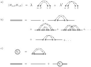
Figure 4: (a) Diagrammatic rules for the ensemble average using Random Matrix Theory. The weight factors depend on the symmetry present: $\lambda^{\prime}=\lambda$ in the presence of time reversal symmetry, while $\lambda^{\prime}$ is reduced in the presence of a weak magnetic field and $\lambda^{\prime}=0$ where time reversal symmetry is fully broken. (b) Expansion of the full matrix propagator in terms of single propagators $1/(\varepsilon+i\pi\nu WW^{\dagger})$, depicted by single lines, and the matrix elements $H_{\alpha\beta}$, depicted by two open circles. (c) Dyson equation for the self energy $\Sigma$.

IV.2.1 Average Green function

We first discuss the calculation of the ensemble average of the Green function, $\langle G^{\rm R}_{ij}(\varepsilon)\rangle$ and $\langle G^{\rm A}_{ij}(\varepsilon)\rangle$. Following the diagrammatic rules laid out in Fig. 4 and keeping diagrams in the non-crossing approximation only,Abrikosov et al. (1963) i.e. diagrams without crossing double lines, one finds that the ensemble averaged Green function $\langle G^{\rm R}_{ij}(\varepsilon)\rangle$ satisfies the Dyson equation

$$\langle G^{\rm R}_{ij}(\varepsilon)\rangle=G^{\rm R}_{0}(\varepsilon)_{ij}+\sum_{k}G^{\rm R}_{0}(\varepsilon)_{ik}\Sigma_{k}\langle G^{\rm R}_{kj}(\varepsilon)\rangle,$$ (68)

where the self energy $\Sigma_{k}$ is

$$\Sigma^{\rm R}_{k}(\varepsilon)=\frac{\lambda_{k}}{M_{k}}\mbox{tr}\,\langle G^{\rm R}_{kk}(\varepsilon)\rangle,$$ (69)

and $G^{\rm R}_{0}(\varepsilon)$ is the solution of Eq. (LABEL:eq:GReq) with $H_{i}=0$. Combining Eqs. (68) and (69) gives a self-consistent equation for $\Sigma^{\rm R}$. In the limit $M_{i}\gg g_{i1}^{\prime}+g_{i2}^{\prime}+\sum_{j\neq i}g_{ij}$, one finds

$$\langle G^{\rm R}_{ij}(\varepsilon)\rangle = \langle G^{\rm A}_{ji}(\varepsilon)\rangle^{\dagger}$$ (70)

$$= -\frac{i\pi}{M_{i}+\Delta_{i}}\tilde{\nu}_{ij}-\sqrt{\frac{\pi^{2}\nu_{i}\nu_{j}}{4M_{i}M_{j}}}t_{ij}$$

$$\mbox{}+\frac{\pi}{2M_{i}^{2}}\left(\pi\nu_{i}\varepsilon-i\mbox{tr}\,\frac{\Delta_{i}}{M_{i}+\Delta_{i}}\right)\tilde{\nu}_{ij},$$

where $\tilde{\nu}_{ij}$ and $t_{ij}$ are given in Eq. (15) and (59) above and $\Delta_{i}$ is an hermitian $M_{i}\times M_{i}$ matrix,

$$\Delta_{i}\,=\,\pi^{2}\nu_{i}\sum_{k\neq i}^{N_{\rm D}}\frac{1}{M_{k}}V_{ik}\nu_{k}V_{ki}+\pi^{2}\nu_{i}\sum_{a=1}^{2}W_{ia}\nu_{a}W_{ai}.$$ (71)

IV.2.2 Classical conductance

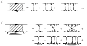
Figure 5: Diffuson ladder (a) and Cooperon ladder (b).

To leading order in the average number $N$ of transmitting channels per dot, the calculation of the average conductance involves the calculation of geometric series involving the ensemble averaged Green functions. Diagrammatically, these geometric series correspond to “ladder diagrams”, as shown in Fig. 5. Such ladders are the equivalent of the “diffuson” propagator in diagrammatic perturbation theory. The building block of the geometric series is

$$\mbox{ tr}\langle G^{\rm R}_{ij}(\varepsilon)\rangle\langle G^{\rm A}_{ji}(\varepsilon^{\prime})\rangle = \frac{\pi^{2}\nu_{i}^{2}}{M_{i}}\delta_{ij}$$

$$\mbox{}-\frac{\pi^{2}\nu_{i}\nu_{j}}{4M_{i}M_{j}}\left[\tilde{g}-i2\pi(\varepsilon-\varepsilon^{\prime})\tilde{\nu}\right]_{ij},$$

where $\tilde{g}_{ij}$ was defined in Eq. (9) above. Summing the geometric series in Fig. 5a then gives the Diffuson matrix

$$D_{ij}(\varepsilon,\varepsilon^{\prime}) = \frac{2M_{i}}{\pi\nu_{i}}\left[\tilde{g}-i2\pi(\varepsilon-\varepsilon^{\prime})\tilde{\nu}\right]^{-1}_{ij}\frac{2M_{j}}{\pi\nu_{j}}.$$ (73)

For the calculation of the mean conductance one also needs a trace that involves the lead indices,

$$D_{ia}^{\prime} = \pi\nu_{a}\mbox{tr}\,\left[W_{ai}\langle G^{\rm R}_{ii}\rangle\langle G^{\rm A}_{ii}\rangle W_{ia}\right]$$ (74)

$$= \pi\nu_{i}\frac{g_{ai}^{\prime}}{4M_{i}},\ \ a=1,2.$$

Combining everything, we then find the leading conductance of the system

$$\langle g\rangle=g_{1\cdot}^{\prime}(\tilde{g}^{-1})_{\cdot\cdot}g_{\cdot 2}^{\prime},$$

which is equation (20) of section II.

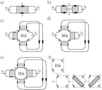
Figure 6: (a) Diagrammatic representation of the leading contribution $g^{\rm cl}$ to the ensemble-averaged conductance $\langle g\rangle$. (b)–(e) Diagrams contributing to the weak localization correction $\delta g^{\rm WL}$. (f) Definition of the Hikami-box used in (c)–(e).

IV.2.3 Weak localization correction

The above calculation gives the conductance to leading order in $g$. A correction to sub-leading order in $g$ is given by a class of diagrams that contains a maximally crossed ladder, as shown in Fig. 5b. These contributions are analogous to the “Cooperon” contributions in diagrammatic perturbation theory.Altshuler and Aronov (1985) The summation of the geometric series promotes the contribution to be of order $1/N$ instead of $1/M$, as is the naive expectations for diagrams that contain one crossed line.

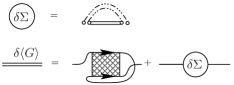
Figure 7: Dyson equation for corrections to $\langle G_{ii}\rangle$ due to the possibility of Cooperon like ladders in the time reversal symmetric case. Double-hatching indicates a retarded-retarded or advanced-advanced pairing. These ladders are parametrically small, and for that reason can also not extend across multiple dots.

In contrast to the diffuson propagator discussed above, the cooperon propagator is sensitive to magnetic flux. Proceeding as before, we find

$$C_{ij}(\varepsilon,\varepsilon^{\prime})\,=\,\frac{2M_{i}}{\pi\nu_{i}}\left[\tilde{g}_{\rm H}+\tilde{g}-2\pi i\tilde{\nu}(\varepsilon-\varepsilon^{\prime})\right]^{-1}_{ij}\frac{2M_{j}}{\pi\nu_{j}},$$ (75)

with $g_{\rm H}$ defined in Eq. (14). For the calculations below, we also need geometric series of Green functions of the same type. These read

$$C_{ij}^{\rm RR}(\varepsilon,\varepsilon^{\prime}) = C_{ij}^{\rm AA}(\varepsilon,\varepsilon^{\prime})^{*}$$ (76)

$$= \frac{1}{16\pi^{2}\nu_{i}\nu_{j}}\Big{(}\big{(}8M_{i}+\tilde{g}_{{\rm H},ii}+\tilde{g}_{ii}$$

$$\mbox{}-i2\pi(\varepsilon+\varepsilon^{\prime})\nu_{i}\big{)}\delta_{ij}-\tilde{g}_{ij}\left(1-\delta_{ij}\right)\Big{)}.~{}~{}~{}~{}$$

Cooperon ladders give a correction to the self-energy appearing in the calculation of the average Green function, as depicted in Fig. 7. Calculation of the self-energy correction $\delta\Sigma_{i}$ to leading order in $g/M$ then gives

$$\delta\Sigma_{i} = \frac{\lambda_{i}}{M_{i}}\mbox{ tr}\left[\langle G^{\rm R}_{ii}\rangle(C^{\rm RR}_{ii}\langle G^{\rm R}_{ii}\rangle+\delta\Sigma_{i})\langle G^{\rm R}_{ii}\rangle\right]$$ (77)

$$= \frac{i}{4\pi\nu_{i}}\mbox{.}$$

As this contribution is already small as $1/M$, one may neglect the effect of a weak magnetic field on this term. The self energy correction $\delta\Sigma$ affects the diffusion ladders as $D\to D+\delta D$, with

$$\delta D_{ij}=-\frac{\pi^{2}\nu_{i}^{2}}{2M_{i}^{2}}\delta_{ij}\mbox{.}$$ (78)

This contribution is depicted in figure 6b.

In the diagrams for the weak localization correction to the conductance, the Cooperon and diffuson propagators are connected in a so-called “Hikami box”.Hikami (1981) In our diagrammatic analysis the analogue of a Hikami box is depicted in figure 6f. We consider the general case of a Hikami box with four energy arguments. We write $\varepsilon_{1}$ ($\varepsilon_{1}^{\prime}$) for the energy argument of the retarded (advanced) matrix propagator on the left side, and $\varepsilon_{2}$ ($\varepsilon_{2}^{\prime}$) for the energy argument of the retarded (advanced) propagator on the right. For the calculation of the weak localization correction one only needs the case of equal arguments, $\varepsilon_{1}=\varepsilon_{1}^{\prime}=\varepsilon_{2}=\varepsilon_{2}^{\prime}$. For dephasing and interaction corrections, some arguments differ. Explicit calculation shows that the Hikami box depends on the combination $\omega=\varepsilon_{1}^{\prime}-\varepsilon_{1}+\varepsilon_{2}^{\prime}-\varepsilon_{2}$ only. Hence we write $B_{ij,kl}(\omega)$, where the indices $i$ and $j$ refer to the left and right (Diffuson) ladders and the indices $k$ and $l$ refer to the bottom and top (Cooperon) ladders.

The calculation is essential but technical; we outline it in the appendix A. The Hikami box $B_{ij,kl}(\omega)$ is zero except where at most two different indices appear,

$$B_{ij,kl}(\omega) = \frac{\pi^{4}\nu_{i}\nu_{j}\nu_{k}\nu_{l}}{16M_{i}M_{j}M_{k}M_{l}}\left[2\pi i\nu_{i}\omega\delta_{ij}\delta_{jk}\delta_{kl}+(\delta_{il}\delta_{jk}+\delta_{ik}\delta_{jl})(\tilde{g}_{ij}+\tilde{g}_{{\rm H},ij}-\tilde{f}_{ij})\right.$$ (79)

$$\left.\mbox{}+(\delta_{ik}\delta_{il}+\delta_{jk}\delta_{jl})\tilde{f}_{ij}+(\delta_{ij}\delta_{ki}+\delta_{ij}\delta_{li})\tilde{f}_{kl}-\delta_{ij}\delta_{kl}\tilde{f}_{ik}\right].$$

For the evaluation of the weak localization correction, one also needs to consider Hikami boxes that are connected to the leads, not only to Diffuson propagators inside the quantum dot network. The two contributions of this type are depicted in figure 6c and d. They are

$$B^{\prime}_{aj,jj} = B^{\prime}_{ja,jj}$$ (80)

$$= -\frac{\pi^{3}\nu_{j}^{3}}{16M_{j}^{3}}f^{\prime}_{aj}.$$

Combining everything, we have (see Fig. 6)

$$\delta g^{\rm WL} = 2D_{1\cdot}^{\prime}D_{\cdot\cdot}\delta D_{\cdot\cdot}D_{\cdot\cdot}D_{\cdot 2}^{\prime}+2\sum_{i,j=1}^{\mathcal{N}_{\rm D}}C_{ij}\left(D_{1\cdot}^{\prime}D_{\cdot\cdot}B^{\prime}_{\cdot 2,ji}+B^{\prime}_{1\cdot,ji}D_{\cdot\cdot}D_{\cdot 2}^{\prime}+D_{1\cdot}^{\prime}D_{\cdot\cdot}B_{\cdot\cdot,ji}(0)D_{\cdot\cdot}D_{\cdot 2}^{\prime}\right),$$ (81)

where $D_{ia}^{\prime}=D_{ai}^{\prime}$ was defined in Eq. (74) above and we have suppressed superscripts as well as inconsequential energy arguments of $D^{\rm RA}(\varepsilon,\varepsilon)$, $C^{\rm RA}(\varepsilon,\varepsilon)$, cf. Eqs. (73), (76). The four terms correspond to the four diagrams b - e of Fig. 6. Substituting our results for the Hikami box $B$, the Cooperon and Diffuson propagators $C$ and $D$, and the interaction propagator $L$, we arrive at Eq. (21) of Sec. II, with the zero-temperature Cooperon $\tilde{c}=(\tilde{g}+\tilde{g}_{\rm H})^{-1}$.

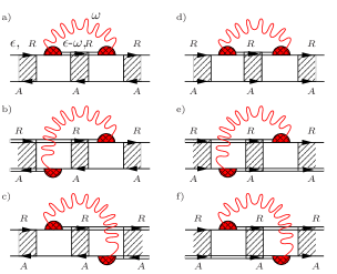
Figure 8: Diagrams for the first-order dephasing correction. Diagrams depicted in (b), (c) and (e), (f) are weighed with a factor $1/2$, in line with Eq. (65). Together (a), (b) and (c) constitute the correction to the Diffuson propagator, which cancels to leading order. Hence the only relevant contributions are the corrections to the Cooperon in (d), (e) and (f). In both cases, complex conjugate contributions exist which are obtained by placing the vertices on the opposite matrix propagation lines.

So far we have not taken into account electron-electron interactions. To lowest order in perturbation theory in the interaction Hamiltonian $\hat{H}_{\rm int}$, the dominant interaction correction to weak localization comes from $\delta g^{\rm deph}$ in Eq. (65). The corresponding diagrams are depicted in Fig. 8. We now calculate that correction. This interaction correction is nonzero only if both interaction vertices appear inside the Cooperon propagator. (This is why this interaction correction does not affect the leading contribution $g_{0}$ to the conductance.)

To calculate the interaction correction, one notices that the interaction vertices are “dressed”, as is shown in Fig. 9. For this case energy arguments may be neglected, as they lead to corrections small in $g/M$. Labeling the dot in which the interaction takes place by the index $\alpha$, the dressed interaction then reads

$$I^{\rm R}_{\alpha,ij} = (I^{\rm A}_{\alpha,ij})^{*}$$ (82)

$$= \mbox{ tr}\left[\langle G^{\rm R}_{ii}\rangle\left(1+\mbox{ tr}\left[\langle G^{\rm R}_{ii}\rangle\langle G^{\rm R}_{ii}\rangle\right]D^{\rm RR}_{ii}\right)\langle G^{\rm R}_{ii}\rangle\langle G^{\rm A}_{ii}\rangle\right]\delta_{\alpha i}\delta_{\alpha j}$$

$$= \frac{\pi\nu_{i}}{2M_{i}}\left(-i2\pi\tilde{\nu}_{ij}\delta_{\alpha i}\right)\frac{\pi\nu_{i}}{2M_{i}}$$

where

$$D_{ij}^{\rm RR}(\varepsilon,\varepsilon^{\prime}) = D_{ij}^{\rm AA}(\varepsilon,\varepsilon^{\prime})^{*}$$ (83)

$$= \frac{1}{16\pi^{2}\nu_{i}\nu_{j}}\Big{[}\big{(}8M_{i}+\tilde{g}_{ii}-i2\pi(\varepsilon+\varepsilon^{\prime})\nu_{i}\big{)}\delta_{ij}-\tilde{g}_{ij}\left(1-\delta_{ij}\right)\Big{]}.$$

The interaction correction $\delta C$ to the equal-energy Cooperon propagator $C(\varepsilon,\varepsilon)$ then becomes

$$\delta C_{ij} = \int d\varepsilon\int\frac{d\omega}{2\pi}\left[-\partial_{\varepsilon}f(\varepsilon)\right]\left[\coth(\omega/2T)+\tanh((\varepsilon-\omega)/2T)\right]\,\sum_{\alpha,\beta=1}^{\mathcal{N}_{\rm D}}\mbox{Im}\,[L^{\rm R}_{\alpha\beta}(\omega)]$$ (84)

$$\mbox{}\times\left[C_{i\cdot}(\varepsilon,\varepsilon)I^{\rm R}_{\alpha,\cdot\cdot}C_{\cdot\cdot}(\varepsilon-\omega,\varepsilon)I^{\rm R}_{\beta,\cdot\cdot}C_{\cdot j}(\varepsilon,\varepsilon)+C_{i\cdot}(\varepsilon-\omega,\varepsilon)I^{\rm A}_{\alpha,\cdot\cdot}C_{\cdot\cdot}(\varepsilon-\omega,\varepsilon-\omega)I^{\rm R}_{\beta,\cdot\cdot}C_{\cdot j}(\varepsilon,\varepsilon-\omega)+\mbox{c.c.}\right].~{}~{}~{}~{}$$

Performing the energy integration and passing to dimensionless propagators, we then find

$$\delta c_{ij} = \int\frac{d\omega}{2\pi}\frac{\omega}{2T\sinh^{2}(\omega/2T)}\sum_{\alpha,\beta=1}^{\mathcal{N}_{\rm D}}\mbox{Im}\,[4\pi^{2}\nu_{\alpha}\nu_{\beta}L^{\rm R}_{\alpha\beta}(\omega)]$$

$$\mbox{}\times\left\{\left(\tilde{g}+\tilde{g}_{\rm H}+i2\pi\omega\tilde{\nu}\right)^{-1}_{i\alpha}\left(\tilde{g}+\tilde{g}_{\rm H}\right)^{-1}_{\alpha\beta}\left(\tilde{g}+\tilde{g}_{\rm H}-i2\pi\omega\tilde{\nu}\right)^{-1}_{\beta j}-\left(\tilde{g}+\tilde{g}_{\rm H}\right)^{-1}_{i\alpha}\left(\tilde{g}+\tilde{g}_{\rm H}+i2\pi\omega\tilde{\nu}\right)^{-1}_{\alpha\beta}\left(\tilde{g}+\tilde{g}_{\rm H}\right)^{-1}_{\beta j}\right.$$

$$\left.\mbox{}+\left(\tilde{g}+\tilde{g}_{\rm H}-i2\pi\omega\tilde{\nu}\right)^{-1}_{i\alpha}\left(\tilde{g}+\tilde{g}_{\rm H}\right)^{-1}_{\alpha\beta}\left(\tilde{g}+\tilde{g}_{\rm H}+i2\pi\omega\tilde{\nu}\right)^{-1}_{\beta j}-\left(\tilde{g}+\tilde{g}_{\rm H}\right)^{-1}_{i\alpha}\left(\tilde{g}+\tilde{g}_{\rm H}-i2\pi\omega\tilde{\nu}\right)^{-1}_{\alpha\beta}\left(\tilde{g}+\tilde{g}_{\rm H}\right)^{-1}_{\beta j}\right\}.$$

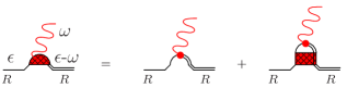
Figure 9: Renormalization of the interaction vertex by ladder diagrams involving Green’s functions of the same type (retarded-retarded or advanced-advanced).

Let us now inspect the integral in Eq. (IV.2.3). The term between brackets $\{\ldots\}$ is proportional to $\omega^{-2}$ if $\omega\gtrsim\hbar/\tau_{\rm D}$, where $\hbar/\tau_{\rm D}\sim g/\nu$ is the inverse dwell time of a dot in the network. Since $\mbox{Im}\,L^{\rm R}(\omega)\propto\omega$ for $\omega\sim\hbar/\tau_{\rm D}$, one thus concludes that the integral in Eq. (IV.2.3) converges at $\omega\sim\min(\hbar/\tau_{\rm D},T)$. We focus on the regime $T\gg\hbar/\tau_{\rm D}$, in which the convergence is at $\omega\sim\hbar/\tau_{\rm D}$. In this regime the inequality $\omega\ll T$ is obeyed for all frequencies $\omega$ contributing to the integral, so that all relevant interaction modes that contribute to dephasing can be described using the classical fluctuation-dissipation theorem. Indeed, one verifies that in this regime the first-order interaction correction (IV.2.3) agrees with the interaction correction to $\tilde{c}$ obtained in the semiclassical framework of Sec. III, taken to first order in the interaction propagator $L$.

Estimating the magnitude of the first-order correction $\delta\tilde{c}_{ij}$ for $T\gg\hbar/\tau_{\rm D}$, we find that $\delta\tilde{c}_{ij}\sim\tilde{c}_{ij}T/T_{\phi}$, where $T_{\phi}\sim\hbar g/\tau_{\rm D}$ [see Eq. (30) above]. This observation has two consequences: First, it implies that the regimes of validity of first-order perturbation theory and the semiclassical approach of Sec. III overlap: Both approaches are valid if $\hbar/\tau_{\rm D}\ll T\ll T_{\phi}$. Second, it implies that interactions give no significant correction to the weak localization correction $\delta g^{\rm WL}$ if $T\lesssim\hbar/\tau_{\rm D}$, so that we may ignore the difference between the fully quantum-mechanical interaction correction $\delta\tilde{c}_{ij}$ of Eq. (IV.2.3) and the semiclassical result in the low-temperature regime $T\lesssim\hbar/\tau_{\rm D}$ within the limiting procedure outlined in Sec. II. (Both approaches give essentially no interaction correction to weak localization at these temperatures.) When combined, these two observations justify the semiclassical considerations of Sec. III, as well as the expressions (21) – (II.2) for the weak localization correction $\delta g^{\rm WL}$ that followed from these considerations.

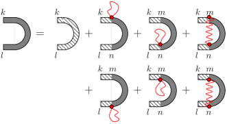
Figure 10: Dyson equation for the Cooperon obtained by perturbation theory in the high temperature limit. The hatched boxes indicate noninteracting Cooperon ladders, while gray shading indicates that interactions are taken into account. Wiggly lines indicate the equal time interaction propagator, which can either connect back to the same propagation line, or to the opposite, time reversed one.

For completeness, we mention that the full temperature dependence of $\delta g^{\rm WL}$ can also be obtained from diagrammatic perturbation theory. Following the above arguments, in the limit $T\gg\hbar/\tau_{\rm D}$ all factors $\coth(\omega/2T)+\tanh(\varepsilon-\omega)/2T$ appearing in the calculation may be replaced by $2T/\omega$, irrespective of the value of $\varepsilon$. This considerably simplifies the calculation, and the $m$ interaction propagators that appear in $m$th order in perturbation theory may then be placed independently of each other along the cooperon ladder. Using Eq. (47) for the interaction propagator and writing the Cooperon ladders (without interaction corrections) in an integral form similar to Eq. (40),

$$\left(\tilde{g}+\tilde{g}_{\rm H}+2\pi i\omega\tilde{\nu}\right)^{-1}\,=\,\left(2\pi\hbar\tilde{\nu}\right)^{-1}\int_{0}^{\infty}d\tau e^{-\tilde{\gamma}\tau-i\omega\tau},$$ (86)

one may perform the frequency integrations. The resulting expression consists solely of time integrations with instantaneous interactions. The remaining combinatorial problem leads to a Dyson equation of the form shown in Fig. 10. Here the first term on the right hand side is the noninteracting Cooperon $\tilde{c}_{kl}=(\tilde{g}+\tilde{g}_{\rm H})^{-1}_{kl}$ and the six other terms are obtained by different placements of the interaction propagators. [Note that where beginning and end are on the same Green’s function line, an additional weight of $1/2$ arises from a factor $\int_{0}^{\infty}d\tau\delta(\tau)=1/2$.] Adding the six different contributions gives a vertex proportional to $(4\pi T/d_{\rm s}\hbar)(\tilde{g}^{-1}_{mm}+\tilde{g}^{-1}_{nn}-2\tilde{g}^{-1}_{mn})$, so that one arrives at the Dyson equation

$$\tilde{c}_{kl}\,=\,\left(\tilde{g}+\tilde{g}_{\rm H}\right)^{-1}_{kl}-\sum_{m,n=1}^{\mathcal{N}_{\rm D}}\left[\left(\Gamma+\Gamma_{\rm H}\right)^{-1}\Gamma_{\phi}\right]_{km,ln}\tilde{c}_{mn},$$ (87)

where $\Gamma$, $\Gamma_{\rm H}$, and $\Gamma_{\phi}$ are rank-four tensors whose definition is given below Eq. (II.2). With a little algebra, one verifies that Eq. (87) is equivalent to the result (22) derived using semiclassical arguments.

Equation (IV.2.3) can also be used to calculate the magnitude of energy quanta $\omega$ exchanged with the fluctuating electromagnetic field in the quantum dots. Hereto, we note that the sum of the second and fourth terms between brackets $\{\ldots\}$ in Eq. (IV.2.3) is proportional to (minus) the probability $p_{1}(\omega)$ for emission or absorption of a photon along the electron’s trajectory, so that

$$p_{1}(\omega) = \frac{1}{g^{\prime}_{1\cdot}\tilde{g}^{-1}_{\cdot\cdot}g^{\prime}_{\cdot 2}}\sum_{\alpha,\beta=1}^{\mathcal{N}_{\rm D}}\frac{\omega}{2\pi T\sinh^{2}{\omega/2T}}\mbox{Im}[4\pi^{2}\nu_{\alpha}\nu_{\beta}L^{\rm R}_{\alpha\beta}(\omega)]\,\mbox{Re}\big{[}g^{\prime}_{1\cdot}\tilde{g}^{-1}_{\cdot\alpha}\left(\tilde{g}+i2\pi\omega\tilde{\nu}\right)^{-1}_{\alpha\beta}\tilde{g}^{-1}_{\beta\cdot}g^{\prime}_{\cdot 2}\big{]}$$ (88)

$$= \frac{16T\pi^{2}}{g^{\prime}_{1\cdot}\tilde{g}^{-1}_{\cdot\cdot}g^{\prime}_{\cdot 2}}\sum_{\alpha,\beta=1}^{\mathcal{N}_{\rm D}}\nu_{\alpha}\tilde{g}^{-1}_{\alpha\beta}\nu_{\beta}\,\mbox{Re}\,[g^{\prime}_{1\cdot}\tilde{g}^{-1}_{\cdot\alpha}\left(\tilde{g}+i2\pi\omega\tilde{\nu}\right)^{-1}_{\alpha\beta}\tilde{g}^{-1}_{\beta\cdot}g^{\prime}_{\cdot 2}],$$

where, in the second equality, we took the limit $T\gg\hbar/\tau_{\rm D}$. The probability that one inelastic scattering event of arbitrary frequency occurs is $P_{1}=\int d\omega p_{1}(\omega)$. Equation (88) is valid as long as $P_{1}\ll 1$, so that first-order perturbation theory is sufficient.

From Eq. (88) we conclude that the energy of photons that are emitted or absorbed is limited by $\min(\hbar/\tau_{\rm D},T)$. The temperature $T_{\phi}$ at which the interaction correction to weak localization becomes relevant is the temperature at which the probability that at least one energy quantum is exchanged becomes of order unity. However, the typical exchanged energy remains of order $\hbar/\tau_{\rm D}$ for all temperatures. This implies that the broadening of the distribution function by inelastic processes is parametrically smaller than the temperature $T$, by a factor $1/g\ll 1$. Transport in the quantum dot network is thus quasielastic for all temperatures. (Inelastic processes become relevant only if $T\gtrsim E_{{\rm Th},i}g^{1/2}$, where $E_{{\rm Th},i}$ is the Thouless energy of an individual quantum dot.)

IV.2.4 Interaction corrections to the conductance

The relevant diagrams for the interaction correction to the conductance $\delta g^{\rm int}$ are shown in Fig. 11. These diagrams do not involve Cooperon propagators. The diagram shown in Fig. 11a is analogous to the ones we have already encountered in calculating the (first-order) dephasing correction to weak localization. It gives an interaction correction to the diffuson propagator $D(\varepsilon,\varepsilon)$ that depends on the frequency $\omega$ of the interaction propagator,

$$\delta D_{\beta\alpha,ij}(\omega)^{(a)} = D_{i\cdot}(\varepsilon,\varepsilon)I^{\rm R}_{\beta,\cdot\cdot}D_{\cdot\cdot}(\varepsilon-\omega,\varepsilon)I^{\rm R}_{\alpha,\cdot\cdot}D_{\cdot j}$$ (89)

$$= -\frac{4M_{i}\nu_{\beta}}{\nu_{i}}\tilde{g}^{-1}_{i\beta}\left(\tilde{g}+i2\pi\omega\tilde{\nu}\right)^{-1}_{\beta\alpha}\tilde{g}^{-1}_{\alpha j}\frac{4M_{j}\nu_{\alpha}}{\nu_{j}}$$

(The frequency $\omega$ will be integrated over in the final expression.) For the remaining diagrams, we need to consider an interaction vertex that connects an advanced and a retarded Green function. Such an interaction vertex is dressed by a Diffuson propagator, which allows the interaction vertex to be placed in a dot different from the one that appears at the outer end of the dressed interaction vertex,

$$\tilde{I}_{\alpha,i}(\omega) = \delta_{\alpha i}+\sum_{k}D_{ik}(\varepsilon-\omega,\varepsilon)\mbox{tr}\,\langle G^{\rm A}_{k\alpha}(\varepsilon)\rangle\langle G^{\rm R}_{\alpha k}(\varepsilon-\omega)\rangle$$ (90)

$$= \frac{4M_{i}\nu_{\alpha}}{\nu_{i}}\left(\tilde{g}+i2\pi\omega\tilde{\nu}\right)^{-1}_{i\alpha}.$$

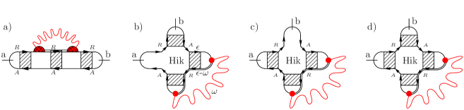
Figure 11: Diagrams contributing to $\delta g^{\rm int}$. The Hikami box is defined in Fig. 6.

With this interaction vertex, the diagrams of Fig. 11b–d (without the outer diffusion ladders) can be represented by Hikami boxes $B_{ij,kl}(\omega)$ and $B^{\prime}_{aj,kl}$ of Eqs. (79) and (80), but with $g_{\rm H}\to 0$ because no Cooperon ladders are involved. Combining the two interaction contributions to the interaction correction we find

$$\delta g^{\rm int} = -4\,\int\frac{d\omega}{2\pi}\left(\frac{\partial}{\partial\omega}\omega\coth\frac{\omega}{2T}\right)\sum_{\alpha\beta}^{N_{\rm D}}\sum_{k,l=1}^{N_{\rm D}}\mbox{Im}\Big{[}L^{\rm A}_{\alpha\beta}(\omega)D_{1\cdot}^{\prime}\delta D_{\beta\alpha,\cdot\cdot}(\omega)^{(a)}D_{\cdot 2}^{\prime}$$ (91)

$$\mbox{}+L^{\rm A}_{\alpha\beta}(\omega)\tilde{I}_{k\alpha}\tilde{I}_{l\beta}\left(B_{1l,\cdot k}^{\prime}D_{\cdot\cdot}D_{\cdot 2}^{\prime}+D_{1\cdot}^{\prime}D_{\cdot\cdot}B^{\prime}_{\cdot l,2k}+D_{1\cdot}^{\prime}D_{\cdot\cdot}B_{\cdot l,\cdot k}(\omega)D_{\cdot\cdot}D_{\cdot 2}^{\prime}\right)\Big{]}.$$

Expressing the propagators in terms of the matrices $\tilde{g}$ and $\tilde{f}$, we find that $\delta g^{\rm int}$ naturally separates into two contributions, which are given by equations (26)–(28) of Sec. II. Both corrections are small for all temperatures, and it is not necessary to consider higher order contributions involving more than one interaction propagator $L$.

V Application to double quantum dot

We now apply the theory of the previous sections to the case of a double quantum dot. There are two cases of interest: A linear configuration, in which each dot is coupled to one reservoir, see Fig. 12a, and a side-coupled configuration, in which both reservoirs are connected to the same quantum dot, see Fig. 12b.

V.1 Linear configuration

The conductance matrix for the linear double quantum dot reads

$$\tilde{g} = \left(\begin{array}[]{cc}g_{11}^{\prime}+g_{12}&-g_{12}\\ -g_{12}&g_{22}^{\prime}+g_{12}\end{array}\right)\mbox{,}$$ (94)

where $g_{11}^{\prime}$ and $g_{22}^{\prime}$ are the dimensionless conductances of the contacts connecting the two dots to the reservoirs, and $g_{12}$ is the dimensionless conductance of the contact between the two dots, see Fig. 12. The form factor matrix $\tilde{f}$ has a similar structure, with $g_{11}^{\prime}$, $g_{22}^{\prime}$, and $g_{12}$ replaced by $f_{11}^{\prime}$, $f_{22}^{\prime}$, and $f_{12}$, respectively. The classical conductance of the system is $G_{\rm cl}=(d_{\rm s}e^{2}/h)g_{\rm cl}$, with

$$g_{\rm cl}^{-1}=g_{11}^{\prime-1}+g_{22}^{\prime-1}+g_{12}^{-1},$$ (95)

see Sec. II, Eq. (20).

V.1.1 Weak localization

The zero temperature weak localization correction to the conductance $\delta G^{\rm WL}=(d_{\rm s}e^{2}/h)\delta g^{\rm WL}$ follows from substitution of the zero-temperature Cooperon $\tilde{c}(0)$ of Eq. (24) into Eq. (21),

$$\frac{\delta g^{\rm WL}}{g_{\rm cl}^{2}} = -\frac{f_{11}^{\prime}/g_{11}^{\prime 2}+f_{12}/g_{12}^{2}}{g_{11}^{\prime}+g_{{\rm H},1}+g_{12}-g_{12}^{2}/(g_{22}^{\prime}+g_{{\rm H},2}+g_{12})}$$

$$\mbox{}-\frac{f_{22}^{\prime}/g_{22}^{\prime 2}+f_{12}/g_{12}^{2}}{g_{22}^{\prime}+g_{{\rm H},2}+g_{12}-g_{12}^{2}/(g_{11}^{\prime}+g_{{\rm H},1}+g_{12})}$$

$$\mbox{}-\frac{2(g_{12}-f_{12})/g_{12}}{(g_{11}^{\prime}+g_{{\rm H},1}+g_{12})(g_{22}^{\prime}+g_{{\rm H},2}+g_{12})-g_{12}^{2}}.$$

Here $g_{{\rm H},2}$ and $g_{{\rm H},1}$ are dimensionless numbers describing the effect of an applied magnetic field, see Eq. (14). The limit of zero magnetic field $g_{{\rm H},2}=g_{{\rm H},1}=0$ agrees with the result obtained previously by Golubev and Zaikin.Golubev and Zaikin (2006) The high-temperature limit of $\delta g^{\rm WL,d}$ of the weak localization correction is found by taking the diagonal contribution $\tilde{c}^{\rm d}$ of Eq. (25) for the Cooperon propagator,

$$\frac{\delta g^{\rm WL,d}}{g_{\rm cl}^{2}} = -\frac{f_{11}^{\prime}/g_{11}^{\prime 2}+f_{12}/g_{12}^{2}}{g_{11}^{\prime}+g_{{\rm H},1}+g_{12}}-\frac{f_{12}/g_{12}^{2}+f_{22}^{\prime}/g_{22}^{\prime 2}}{g_{22}^{\prime}+g_{{\rm H},2}+g_{12}}.$$

Note that $|\delta g_{\rm WL}^{\rm d}|<|\delta g_{\rm WL}|$. The remainder of the weak localization correction, $\delta g^{\rm WL}-\delta g^{\rm WL,d}$, is temperature dependent because of dephasing from electron-electron interactions. Taking the temperature-dependent Cooperon from Eq. (22), we find that the temperature dependence of the full matrix $\tilde{c}(T)$ is encoded in a single scalar function $f(T)$,

$$\tilde{c}(T)=\tilde{c}(0)-[\tilde{c}(0)-\tilde{c}^{\rm d}]f(T).$$ (98)

Equation (98) immediately implies that

$$\delta g^{\rm WL}(T)=\delta g^{\rm WL,d}+[\delta g^{\rm WL}(0)-\delta g^{\rm WL,d}][1-f(T)],$$ (99)

where $\delta g^{\rm WL}(0)$ and $\delta g^{\rm WL,d}$ are given in Eqs. (LABEL:eq:ddwl) and (V.1.1), respectively. In the regime where temperature is large enough for dephasing effects to give a sizeable correction to the weak localization correction to the conductance, we obtain $f(T)$ from Eq. (22),

$$f(T)=\frac{T}{T_{\phi}+T},$$ (100)

with

$$\frac{T_{\phi}}{d_{\rm s}}=\frac{\hbar(\tau_{1}+\tau_{2})(g_{11}^{\prime}g_{22}^{\prime}+g_{11}^{\prime}g_{12}+g_{22}^{\prime}g_{12})}{4\pi\tau_{+}\tau_{-}(g_{11}^{\prime}+g_{22}^{\prime})}.$$ (101)

Here $\tau_{1}$ and $\tau_{2}$ are the (classical) dwell times of the two dots, modified for the presence of a magnetic field,

$$\tau_{1} = \frac{2\pi\hbar\nu_{1}}{g_{11}^{\prime}+g_{{\rm H},1}+g_{12}}\mbox{, }\,\tau_{2}\,=\,\frac{2\pi\hbar\nu_{2}}{g_{22}^{\prime}+g_{{\rm H},2}+g_{12}},$$ (102)

whereas $\tau_{\pm}$ are time scales representing the relaxation of symmetric ($+$) or antisymmetric ($-$) charge configurations in the double dot,

$$\frac{1}{\tau_{\pm}}=\frac{1}{2\tau_{1}}+\frac{1}{2\tau_{2}}\mp\frac{1}{2}\sqrt{\left(\frac{1}{\tau_{1}}-\frac{1}{\tau_{2}}\right)^{2}+\frac{g_{12}^{2}}{\pi^{2}\hbar^{2}\nu_{1}\nu_{2}}}.$$ (103)

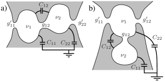
Figure 12: Schematic drawings of two double quantum dots. Panel (a) shows a linear configuration; Panel (b) shows a side-coupled configuration.

It is instructive to compare Eq. (100) with the expression for $f(T)$ obtained in first-order perturbation theory,

$$f(T) = \int\frac{d\omega}{2\pi}\frac{\omega/2T}{\sinh^{2}(\omega/2T)}\frac{2\omega^{2}}{(1+\omega^{2}\tau_{+}^{2}/\hbar^{2})(1+\omega^{2}\tau_{-}^{2}/\hbar^{2})}\,$$

$$\mbox{}\times\frac{\tau_{+}^{3}\tau_{-}^{3}}{\hbar^{4}\tau_{1}\tau_{2}}\mbox{Im}\,[L^{\rm R}_{11}(\omega)+L^{\rm R}_{22}(\omega)-2L^{\rm R}_{12}(\omega)].$$

The integral in Eq. (LABEL:eq:fT) converges for frequencies $\omega/\hbar$ of order $\tau_{\pm}^{-1}$. For these frequencies, we may neglect the capacitance $C$ in the expression for the interaction propagator $L$ since $C/e^{2}\ll\nu$. The resulting frequency integration yields

$$f(T) = \frac{2\pi T\tau_{+}\tau_{-}}{3\hbar(\tau_{+}-\tau_{-})}\frac{T}{T_{\phi}}$$ (105)

$$\mbox{}\times\left[{\cal F}_{1}(2\pi T\tau_{-}/\hbar)-{\cal F}_{1}(2\pi T\tau_{+}/\hbar)\right]$$

where

$${\cal F}_{1}(x)=\frac{3}{x^{2}}\left\{\frac{1}{x}\left[2\psi^{\prime}\left(\frac{1}{x}\right)-x^{2}\right]-2\right\},$$ (106)

$\psi^{\prime}$ being the derivative of the digamma function. With the asymptotic behavior of ${\cal F}_{1}(x)$,

$${\cal F}_{1}(x)=\left\{\begin{array}[]{ll}1-\frac{1}{5}x^{2}+\frac{1}{7}x^{4}+\ldots,&\,x\ll 1,\\ \frac{3}{x}-\frac{6}{x^{2}}+\frac{\pi^{2}}{x^{3}}+\ldots,&\,x\gg 1,\end{array}\right.$$ (107)

we identify three different regimes for the temperature dependence of the dephasing correction:

$$f(T)=\frac{1}{15}\tau_{+}\tau_{-}(\tau_{+}+\tau_{-})\left(\frac{2\pi T}{\hbar}\right)^{3}\frac{T}{T_{\phi}}$$ (108)

if $T\ll\hbar/\tau_{+}$,

$$f(T)=\frac{2\pi T\tau_{-}}{3\hbar}\frac{T}{T_{\phi}}$$ (109)

if $\hbar/\tau_{+}\ll T\ll\hbar/\tau_{-}$, and

$$f(T)=T/T_{\phi}$$ (110)

if $\hbar/\tau_{-}\ll T$, where $T_{\phi}$ is given by Eq. (101) above. The intermediate temperature regime exists only if $\tau_{+}\gg\tau_{-}$. A comparison of Eq. (110) with Eqs. (100) shows that the two expressions for $f(T)$ agree in the temperature regime $\hbar/\tau_{-}\ll T\ll T_{\phi}$ where both expressions are valid. It is in this temperature regime that the factor $(\omega/2T)/\sinh^{2}(\omega/2T)$ in Eq. (LABEL:eq:fT) can be approximated by $2T/\omega$, which is the appropriate weight appearing in the classical fluctuation-dissipation theorem.

It should be noted that the low temperature corrections, Eqs. (108) and (109), result in contributions to the conductance of order $\mathcal{O}(1/g)$. Such contributions are beyond the accuracy achieved in the limiting procedure outlined in Sec. II. Further contributions of the same order might be obtained by calculating, e.g., weak localization corrections to the interaction corrections $\delta g^{{\rm int},1}$ and $\delta g^{{\rm int},2}$. For disordered metals such contributions have been considered explicitly in Ref. Aleiner et al., 1999.

The above equations take a simpler form in the limiting cases of large and small interdot coupling $g_{12}$ and of a large magnetic field. For small interdot coupling $g_{12}\ll\min(g_{11}^{\prime},g_{22}^{\prime})$, one has

$$\delta g^{\rm WL} = -\frac{f_{11}^{\prime}g_{12}^{2}+f_{12}g_{11}^{\prime 2}}{g_{11}^{\prime 2}(g_{11}^{\prime}+g_{{\rm H},1})}-\frac{f_{22}^{\prime}g_{12}^{2}+f_{12}g_{22}^{\prime 2}}{g_{22}^{\prime 2}(g_{22}^{\prime}+g_{{\rm H},2})}$$ (111)

$$\mbox{}-\frac{2(g_{12}-f_{12})g_{12}}{(g_{11}^{\prime}+g_{{\rm H},1})(g_{22}^{\prime}+g_{{\rm H},2})}\frac{T_{\phi}}{T_{\phi}+T},~{}~{}~{}~{}$$

$$\frac{T_{\phi}}{d_{\rm s}} = g_{11}^{\prime}g_{22}^{\prime}\frac{(g_{11}^{\prime}+g_{{\rm H},1})\nu_{1}^{-1}+(g_{22}^{\prime}+g_{{\rm H},2})\nu_{2}^{-1}}{8\pi^{2}(g_{11}^{\prime}+g_{22}^{\prime})},~{}~{}~{}~{}$$ (112)

so that only a small part of the total weak localization correction is temperature dependent. In the limit of a large interdot conductance, $g_{12}\gg\max(g_{11}^{\prime},g_{22}^{\prime},g_{{\rm H},1},g_{{\rm H},2})$, the full weak localization correction acquires a temperature dependence,

$$\delta g^{\rm WL} = -\frac{g_{22}^{\prime 2}f_{11}^{\prime}+g_{11}^{\prime 2}f_{22}^{\prime}}{(g_{11}^{\prime}+g_{22}^{\prime})^{2}(g_{11}^{\prime}+g_{{\rm H},1}+g_{22}^{\prime}+g_{{\rm H},2})}$$

$$\mbox{}\times\frac{T_{\phi}}{T_{\phi}+T},$$

$$\frac{T_{\phi}}{d_{\rm s}} = g_{12}\frac{(g_{11}^{\prime}+g_{{\rm H},1}+g_{22}^{\prime}+g_{{\rm H},2})(\nu_{1}^{-1}+\nu_{2}^{-1})}{8\pi^{2}}.~{}~{}~{}~{}$$ (113)

Finally, in the limit of large magnetic field, $g_{{\rm H},1},g_{{\rm H},2}\gg\max(g_{11}^{\prime},g_{22}^{\prime},g_{12})$, we have

$$\delta g^{\rm WL} = -g_{\rm cl}^{2}\frac{f_{11}^{\prime}/g_{11}^{\prime 2}+f_{12}/g_{12}^{2}}{g_{{\rm H},1}}-g_{\rm cl}^{2}\frac{f_{22}^{\prime}/g_{22}^{\prime 2}+f_{12}/g_{12}^{2}}{g_{{\rm H},2}}$$ (114)

$$\mbox{}-g_{\rm cl}^{2}\frac{g_{12}-f_{12}}{g_{12}g_{{\rm H},1}g_{{\rm H},2}}\frac{T_{\phi}}{T_{\phi}+T},$$

$$\frac{T_{\phi}}{d_{\rm s}} = \frac{g_{12}}{8\pi^{2}}\left(g_{{\rm H},1}\nu_{1}^{-1}+g_{{\rm H},2}\nu_{2}^{-1}\right).$$ (115)

A special case of two weakly coupled quantum dots ($g_{12}\ll g_{11}^{\prime},g_{22}^{\prime}$) with tunneling contacts ($f_{11}^{\prime}\ll g_{11}^{\prime}$, $f_{22}^{\prime}\ll g_{22}^{\prime}$, $f_{12}\ll g_{12}$) has been considered recently by Golubev and Zaikin.Golubev and Zaikin (2007) While our calculation agrees with that of Ref. Golubev and Zaikin, 2007 in the high temperature regime $T\gg T_{\phi}$, significant differences appear in the low temperature limit. In particular, Golubev and Zaikin find a finite dephasing correction to weak localization at zero temperature, whereas we find no such effect. A similar discrepancy has been found previously in the context of dephasing from the electron-electron interaction in disordered metals.Golubev and Zaikin (1998); Aleiner et al. (1999) In this case the neglect of recoil effects in the influence functional approach used by Golubev and Zaikin has been identified as the cause of the problem.von Delft (2005) This causes an ultraviolet divergence, which does not appear in the perturbation theory, where it is avoided by the $\tanh$-term in the factor $\coth({\omega/2T})+\tanh{((\varepsilon-\omega)/2T)}$ that sets the magnitude of the dephasing correction at low temperatures, see, e.g., Eq. (65) and Refs. Aleiner et al., 1999; von Delft, 2005. (Neglect of recoil amounts to neglecting the $\omega$-dependence of the argument of the $\tanh$, which causes this factor to no longer approach zero at large frequencies $\omega$.) We believe that the discrepancy between our result and that of Ref. Golubev and Zaikin, 2007 has the same origin.

V.1.2 Interaction corrections

The interaction corrections $\delta g^{{\rm int},1}$ and $\delta g^{{\rm int},2}$ do not depend on the magnetic field. Hence, the relevant time scales do not involve $g_{{\rm H},1}$ and $g_{{\rm H},2}$, and we define

$$\tau_{i}=\frac{2\pi\hbar\nu_{i}}{g_{ii}^{\prime}+g_{12}},\ \ i=1,2.$$ (116)

Again, we introduce time scales $\tau_{\pm}$ related to $\tau_{1}$ and $\tau_{2}$ as in Eq. (103) above. For the first interaction correction $\delta g^{{\rm int},1}$ we then find

$$\delta g^{{\rm int},1} = \frac{g_{\rm cl}^{3}}{d_{\rm s}g_{11}^{\prime}g_{12}g_{22}^{\prime}}\int d\omega\left(\frac{\partial}{\partial\omega}\omega\coth\frac{\omega}{2T}\right)$$ (117)

$$\times\mbox{Im}\frac{(\tau_{+}+\tau_{-})/\hbar}{(1+i\omega\tau_{+}/\hbar)(1+i\omega\tau_{-}/\hbar)}.$$

This result was obtained previously in Ref. Brouwer and Kupferschmidt, 2007 for the symmetric case $g_{11}^{\prime}=g_{22}^{\prime}$, $\nu_{1}=\nu_{2}$ and in Ref. Golubev and Zaikin, 2004a for the case $g_{11}^{\prime}=g_{22}^{\prime}=g_{12}$, $\nu_{1}=\nu_{2}$. The frequency integral in Eq. (117) can be evaluated in terms of digamma functions. We have

$$\int d\omega\left(\frac{\partial}{\partial\omega}\omega\coth\frac{\omega}{2T}\right)\mbox{Im}\left[\frac{1}{(1+i\omega\tau_{\alpha}/\hbar)(1+i\omega\tau_{\beta}/\hbar)}\right]=\frac{2\hbar}{\tau_{\alpha}-\tau_{\beta}}\left[{\cal F}_{2}\left(\frac{\hbar}{2\pi T\tau_{\alpha}}\right)-{\cal F}_{2}\left(\frac{\hbar}{2\pi T\tau_{\beta}}\right)\right],~{}~{}~{}~{}~{}~{}~{}~{}$$ (118)

where

$${\cal F}_{2}(x)\,=\,\psi(1+x)+x\psi^{\prime}(1+x)$$ (119)

and $\psi(x)$ is the digamma function.Golubev and Zaikin (2004a) From the asymptotic behavior of ${\cal F}_{2}$,

$${\cal F}_{2}(x)=\left\{\begin{array}[]{ll}-\gamma+\frac{\pi^{2}}{3}x-3\zeta(3)x^{2}+\ldots,&\,x\ll 1,\\ 1+\ln x+\frac{1}{12x^{2}}+\ldots,&\,x\gg 1,\end{array}\right.$$ (120)

with $\gamma$ the Euler-Mascheroni constant, we obtain the high and low temperature limit of the interaction correction $\delta g^{{\rm int},1}$

$$\delta g^{{\rm int},1}=-\frac{2g_{\rm cl}^{3}}{d_{\rm s}g_{11}^{\prime}g_{12}g_{22}^{\prime}}\times\left\{\begin{array}[]{ll}\displaystyle{\frac{\tau_{+}+\tau_{-}}{\tau_{+}-\tau_{-}\vphantom{M^{M}_{M}}}\ln\frac{\tau_{+}}{\tau_{-}}},&T\ll\hbar/\tau_{\pm},\\ \displaystyle{\frac{\pi\hbar(\tau_{+}+\tau_{-})\vphantom{M^{M}_{M}}}{6T\tau_{+}\tau_{-}}},&T\gg\hbar/\tau_{\pm}.\end{array}\right.$$ (121)

The second interaction correction $\delta g^{{\rm int},2}$ is expressed in terms of interaction-induced shifts $\delta g_{11}^{\prime}$, $\delta g_{22}^{\prime}$, and $\delta g_{12}$ to the conductances $g_{11}^{\prime}$, $g_{22}^{\prime}$, and $g_{12}$, respectively, see Eq. (27). In contrast to the interaction correction $\delta g^{{\rm int},1}$ considered above, the frequency integrations needed to calculate $\delta g_{11}^{\prime}$, $\delta g_{22}^{\prime}$, and $\delta g_{12}$ converge only if we account for the finite (nonzero) capacitances of the quantum dots, see Eq. (28). [The integration in Eq. (28) diverges logarithmically if the limit $C_{ii}/e^{2}\nu_{i}\to 0$ is taken.]

Below we give explicit expressions for the case of a symmetric double dot only, $g_{11}^{\prime}=g_{22}^{\prime}=g^{\prime}$, $f_{11}^{\prime}=f_{22}^{\prime}=f^{\prime}$, $\nu_{1}=\nu_{2}$, and $C=C_{11}=C_{22}$. In this case, the logarithmic divergence of the integration in Eq. (II.2) is cut off at the inverse of the charge-relaxation times,

$$\tau_{\rm c+} = \frac{\tau_{+}}{d_{\rm s}e^{2}\nu/C},\ \ \tau_{\rm c-}=\frac{\tau_{-}}{d_{\rm s}e^{2}\nu/(C+2C_{12})}\mbox{,}~{}~{}~{}~{}~{}$$ (122)

and the corrections $\delta g_{11}^{\prime}=\delta g_{22}^{\prime}=\delta g^{\prime}$ and $\delta g_{12}$ are found to be

$$\delta g^{\prime} = \frac{g^{\prime}-f^{\prime}}{d_{\rm s}g^{\prime}}\sum_{\sigma=\pm}\frac{\tau_{\sigma}}{\tau_{+}}\left[{\cal F}_{2}\left(\frac{\hbar}{2\pi T\tau_{\sigma}}\right)-{\cal F}_{2}\left(\frac{\hbar}{2\pi T\tau_{{\rm c}\sigma}}\right)\right],$$ (123)

$$\delta g_{12} = \frac{2(g_{12}-f_{12})}{d_{\rm s}g_{12}}\frac{\tau_{+}-\tau_{-}}{\tau_{+}}\left[{\cal F}_{2}\left(\frac{1}{2\pi T\tau_{-}/\hbar}\right)-{\cal F}_{2}\left(\frac{1}{2\pi T\tau_{{\rm c}-}/\hbar}\right)\right]\mbox{.}$$ (124)

For the case $g^{\prime}=g_{12}$, $f^{\prime}=f_{12}$ and $C_{12}=0$, Eqs. (123) and (124) agree with results obtained previously in Ref. Golubev and Zaikin, 2004a. [ The result of Ref. Golubev and Zaikin, 2004a differs from Eqs. (123) and (124) if $C_{12}>0$ because Ref. Golubev and Zaikin, 2004a includes cross capacitances between each dot and adjacent reservoir of the same magnitude as the cross capacitance $C_{12}$ between the two dots.] Equation (123) simplifies to the renormalization of the contact conductance for a single quantum dot in the limit $g_{12}\to\infty$.Golubev and Zaikin (2004b); Brouwer et al. (2005a, b) Again making use of the asymptotic behavior of the digamma function, we find that the above expressions simplify to

$$\delta g^{\prime}=-\frac{g^{\prime}-f^{\prime}}{d_{\rm s}g^{\prime}}\times\left\{\begin{array}[]{ll}\displaystyle{\ln\frac{\tau_{+}}{\tau_{{\rm c}+}}+\frac{\tau_{-}}{\tau_{+}}\ln\frac{\tau_{-}}{\tau_{{\rm c}-}}},&T\ll\hbar/\tau_{\pm},\\ \displaystyle{\ln\frac{e^{1+\gamma}}{2\pi T\tau_{{\rm c}+}}+\frac{\tau_{-}}{\tau_{+}}\ln\frac{e^{1+\gamma}}{2\pi T\tau_{{\rm c}-}}},&\hbar/\tau_{\pm}\ll T\ll\hbar/\tau_{{\rm c}\pm},\\ \displaystyle{\frac{\pi\hbar}{6T\tau_{+}}\left(\frac{\tau_{+}}{\tau_{{\rm c}+}}+\frac{\tau_{-}}{\tau_{{\rm c}-}}\right)},&\hbar/\tau_{{\rm c}\pm}\ll T,\end{array}\right.$$ (125)

$$\delta g_{12}=-\frac{4(g_{12}-f_{12})}{d_{\rm s}g_{12}}\frac{\tau_{+}-\tau_{-}}{\tau_{+}}\times\left\{\begin{array}[]{ll}\displaystyle{\ln\frac{\tau_{-}}{\tau_{{\rm c}-}}},&T\ll\hbar/\tau_{\pm},\\ \displaystyle{\ln\frac{e^{1+\gamma}}{2\pi T\tau_{{\rm c}-}}},&\hbar/\tau_{-}\ll T\ll\hbar/\tau_{{\rm c}-},\\ \displaystyle{\frac{\pi\hbar}{6T\tau_{{\rm c}-}}},&\hbar/\tau_{{\rm c}\pm}\ll T.\end{array}\right.$$ (126)

V.2 Side-coupled quantum dot

For the side-coupled double dot configuration of figure 12 the structure of the weak localization correction and the interaction corrections is essentially the same as for the linear configurations. The classical conductance is

$$g_{\rm cl}^{-1}=g_{11}^{\prime-1}+g_{12}^{\prime-1}.$$ (127)

The weak localization correction to the conductance is

$$\delta g^{\rm WL} = -\frac{f_{22}^{\prime}g_{11}^{\prime 2}+f_{11}^{\prime}g_{12}^{\prime 2}}{(g_{11}^{\prime}+g_{12}^{\prime})^{2}(g_{11}^{\prime}+g_{12}^{\prime}+g_{12}+g_{{\rm H},1})}\left\{1+\frac{g_{12}^{2}[1-f(T)]}{(g_{11}^{\prime}+g_{12}^{\prime}+g_{{\rm H},1})(g_{12}+g_{{\rm H},2})+g_{12}g_{{\rm H},2}}\right\},$$

where $f(T)=T/(T_{\phi}+T)$,

$$\frac{T_{\phi}}{d_{\rm s}}\,=\,\frac{1}{4\pi}\frac{\tau_{1}+\tau_{2}}{\tau_{+}\tau_{-}}g_{12},$$ (128)

and

$$\tau_{1} = \frac{2\pi\hbar\nu_{1}}{g_{11}^{\prime}+g_{12}^{\prime}+g_{{\rm H},1}+g_{12}}\mbox{, }\,\tau_{2}\,=\,\frac{2\pi\hbar\nu_{2}}{g_{12}+g_{{\rm H},2}},~{}~{}~{}$$ (129)

with $\tau_{\pm}$ given in terms of $\tau_{1}$ and $\tau_{2}$ as in Eq. (103).

Again, it is instructive to compare to what one finds to lowest order in perturbation theory. The result is identical to Eq. (105), where $\tau_{1},\tau_{2}$ and $T_{\phi}$ are those of the side-coupled system, Eqs. (128) and (129). Simplified expressions for the function $f(T)$ in the regimes $T\ll\hbar/\tau_{+}$, $\hbar/\tau_{+}\ll T\ll\hbar/\tau_{-}$, and $\hbar/\tau_{-}\ll T$ are as in Eqs. (108)–(110).

In the limit of small interdot coupling $g_{12}\to 0$ only a very small fraction of the weak localization correction is temperature dependent,

$$\delta g^{\rm WL} = -\frac{f_{22}^{\prime}g_{11}^{\prime 2}+f_{11}^{\prime}g_{12}^{\prime 2}}{(g_{11}^{\prime}+g_{12}^{\prime})^{2}(g_{11}^{\prime}+g_{12}^{\prime}+g_{{\rm H},1})}$$

$$\mbox{}\times\left[1+\frac{g_{12}^{2}}{(g_{11}^{\prime}+g_{12}^{\prime}+g_{{\rm H},1})g_{{\rm H},2}}\frac{T_{\phi}}{T_{\phi}+T}\right],$$

$$\frac{T_{\phi}}{d_{\rm s}} = \frac{g_{12}}{8\pi^{2}}\left[(g_{11}^{\prime}+g_{12}^{\prime}+g_{{\rm H},1})\nu_{1}^{-1}+g_{{\rm H},2}\nu_{2}^{-1}\right].~{}~{}~{}~{}~{}$$ (130)

In the opposite limit of a large interdot conductance the entire weak localization correction is temperature dependent. In this limit there is no difference between the linear and side-coupled configurations, and one finds that $\delta g^{\rm WL}$ is given by Eq. (113) above, with $g_{22}^{\prime}$ replaced by $g_{12}^{\prime}$. Finally, in the limit of large magnetic fields we find

$$\delta g_{\rm WL} = -\frac{g_{12}^{\prime 2}f_{11}^{\prime}+g_{11}^{\prime 2}f_{22}^{\prime}}{(g_{11}^{\prime}+g_{12}^{\prime})^{2}g_{{\rm H},1}}\left(1+\frac{g_{12}^{2}}{g_{{\rm H},1}g_{{\rm H},2}}\frac{T_{\phi}}{T_{\phi}+T}\right),$$

$$\frac{T_{\phi}}{d_{\rm s}} = \frac{g_{12}}{8\pi^{2}}\left(g_{{\rm H},1}\nu_{1}^{-1}+g_{{\rm H},2}\nu_{2}^{-1}\right).$$ (131)

With a side coupled quantum dot, the interaction correction $\delta g^{{\rm int},1}$ to the conductance vanishes. The interaction correction $\delta g^{{\rm int},2}$ coming from the renormalization of the contact conductances remains. The detailed expressions are rather lengthy and will not be reported here.

VI Conclusion

We have calculated the quantum corrections to the conductance of a network of quantum dots, including the full dependence on temperature and magnetic field. Our results are valid in the limit that the quantum dot network has conductance $g$ much larger than the conductance quantum, so that the quantum corrections are small in comparison to the classical conductance, and in the limit that the electron dynamics inside each quantum dot is ergodic. Following the literature, we separated the quantum corrections into the weak localization correction $\delta g^{\rm WL}$ and two interaction corrections $\delta g^{{\rm int},1}$, $\delta g^{{\rm int},2}$. Our results for the interaction corrections agree with previous calculations of $\delta g^{{\rm int},1}$ and $\delta g^{{\rm int},2}$ by Golubev and ZaikinGolubev and Zaikin (2004a) for a linear array of quantum dots, and are closely related to similar interaction corrections in a granular metal, see Ref. Beloborodov et al., 2003a. Our result for $\delta g^{\rm WL}$ agrees with the literature in the limit of zero temperatureCampagnano and Nazarov (2006); Golubev and Zaikin (2006) and in the high temperature limit,Blanter et al. (2006) but we are not aware of a calculation of the full temperature dependence of $\delta g^{\rm WL}$ in the literature. (The exception is a calculation of $\delta g^{\rm WL}$ for a double quantum dot by Golubev and Zaikin which, however, gives an unphysical result in the limit of zero temperature.Golubev and Zaikin (2007))

We have formulated our final results in such a way that the evaluation of quantum corrections for a network of a relatively small number $\mathcal{N}_{\rm D}$ of quantum dots does not require more than the inversion of an $\mathcal{N}_{\rm D}$-dimensional matrix. All quantum corrections to the conductance can be expressed in terms of the inter-dot conductances, form factors, and the capacitances only. In principle, these parameters can be measured independently. This makes a small quantum dot network an ideal model system to compare theory and experiment, and to unambiguously identify the mechanisms responsible for dephasing. (Capacitances and form factors play a role only if the dots are connected via non-ideal contacts in which one or more transmission eigenvalues are smaller than one. For lateral quantum dot networks defined in semiconductor heterostructures, contacts are typically ballistic, and the only relevant parameters are the quantized conductances of the contacts between the quantum dots.)

The simplest example of a small quantum dot network is a ‘double quantum dot’, which consists of two quantum dots coupled to each other and to electron reservoirs via point contacts. Several groups have reported transport measurements on such double dots,Waugh et al. (1995); Livermore et al. (1996); Oosterkamp et al. (1998); Holleitner et al. (2001) or even on triple dots.Waugh et al. (1995) (Double quantum dots also play a prominent role in recent attempts to achieve quantum computation.van der Wiel et al. (2003) However, the dots used in these experiments typically hold one or two electrons each and can not be described by random matrix theory.) Although, in principle, the contact conductances in lateral double and triple quantum dot networks are fully tunable, the experiments of Refs. Waugh et al., 1995; Livermore et al., 1996; Oosterkamp et al., 1998; Holleitner et al., 2001 were performed for the case that the devices are weakly coupled to the source and drain reservoirs. In that limit, transport is dominated by the Coulomb blockade. Our theory applies to the opposite regime in which all dots in the network are open, well coupled to source and/or drain reservoirs. We hope that the availability of quantitative theoretical predictions will lead to renewed experimental interest in quantum transport through open quantum dots.

Appendix A Hikami Box calculation

In this appendix we provide details on the derivation of Eqs. (79) and (80) of Sec. IV. The explicit expression for the Hikami box is an essential part of the calculation of the quantum corrections to the conductance, but we have not found the explicit expression of Eq. (79), nor its derivation, in the literature.

We refer to the text surrounding Eq. (79) for the notations used in this appendix. In general, the Hikami box $B_{ij,kl}(\omega)$ will be nonzero only if the four indices span at most two adjacent quantum dots. We here show the calculation of $B_{ii,ii}(\omega)$. There are three contributions to $B_{ii,ii}(\omega)$, which are shown in Fig. 13ii,ii a–c. They read

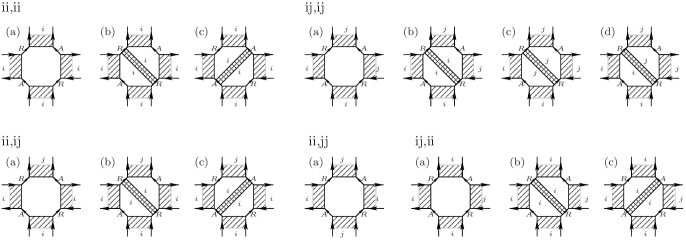
Figure 13: Diagrammatic depiction of Hikami boxes. Different diagrams contribute depending on where the cooperon and diffuson like ladders end and begin.

$$B_{ii,ii}^{(a)}(\omega) = \mbox{ tr}\left[\langle G^{\rm R}_{ii}(\varepsilon_{1})\rangle\langle G^{\rm A}_{ii}(\varepsilon_{2}^{\prime})\rangle\langle G^{\rm R}_{ii}(\varepsilon_{2})\rangle\langle G^{\rm A}_{ii}(\varepsilon_{1}^{\prime})\rangle\right]$$ (132)

$$= \frac{\pi^{4}\nu_{i}^{4}}{M_{i}^{3}}\left(1+\frac{i\pi\nu_{i}(\varepsilon_{1}-\varepsilon_{1}^{\prime}+\varepsilon_{2}-\varepsilon_{2}^{\prime})}{2M_{i}}+\mbox{tr}\,\left[\frac{-2\Delta_{i}(M_{i}-\Delta_{i})}{(M_{i}+\Delta_{i})^{3}}+\frac{\Delta_{i}^{4}}{M_{i}(M_{i}+\Delta_{i})^{4}}\right]\right),$$

$$B_{ii,ii}^{(b)}(\omega) = \left(\mbox{ tr}\left[\langle G^{\rm R}_{ii}(\varepsilon_{1})\rangle\langle G^{\rm A}_{ii}(\varepsilon_{2}^{\prime})\rangle\langle G^{\rm R}_{ii}(\varepsilon_{2})\right]\right)C^{\rm RR}_{ii}(\varepsilon_{1},\varepsilon_{2})\left(\mbox{ tr}\left[\langle G^{\rm R}_{ii}(\varepsilon_{1})\rangle\langle G^{\rm R}_{ii}(\varepsilon_{2})\langle G^{\rm A}_{ii}(\varepsilon_{1}^{\prime})\rangle\right]\right)$$ (133)

$$= -\frac{\pi^{4}\nu_{i}^{4}}{2M_{i}^{3}}\left(1+\frac{\tilde{g}_{ii}-\tilde{g}_{{\rm H},ii}+i2\pi(3\varepsilon_{1}-2\varepsilon_{1}^{\prime}+3\varepsilon_{2}-2\varepsilon_{2}^{\prime})}{8M_{i}}+\frac{1}{M_{i}}\mbox{ tr}\left[\frac{\Delta_{i}^{3}-3M_{i}^{2}\Delta_{i}}{(M_{i}+\Delta_{i})^{3}}\right]\right),$$

$$B_{ii,ii}^{(c)}(\omega) = \left(\mbox{ tr}\left[\langle G^{\rm R}_{ii}(\varepsilon_{1})\rangle\langle G^{\rm A}_{ii}(\varepsilon_{2}^{\prime})\rangle\langle G^{\rm A}_{ii}(\varepsilon_{1}^{\prime})\right]\right)C^{\rm AA}_{ii}(\varepsilon_{2}^{\prime},\varepsilon_{1}^{\prime})\left(\mbox{ tr}\left[\langle G^{\rm A}_{ii}(\varepsilon_{2}^{\prime})\rangle\langle G^{\rm R}_{ii}(\varepsilon_{2})\rangle\langle G^{\rm A}_{ii}(\varepsilon_{1}^{\prime})\right]\right)$$ (134)

$$= -\frac{\pi^{4}\nu_{i}^{4}}{2M_{i}^{3}}\left(1+\frac{\tilde{g}_{ii}-\tilde{g}_{{\rm H},ii}+i2\pi(2\varepsilon_{1}-3\varepsilon_{1}^{\prime}+2\varepsilon_{2}-3\varepsilon_{2}^{\prime})}{8M_{i}}+\frac{1}{M_{i}}\mbox{ tr}\left[\frac{\Delta_{i}^{3}-3M_{i}^{2}\Delta_{i}}{(M_{i}+\Delta_{i})^{3}}\right]\right),$$

where the $M_{i}\times M_{i}$ matrix $\Delta_{i}$ was defined in Eq. (71) above and $\omega=\varepsilon_{1}^{\prime}-\varepsilon_{1}+\varepsilon_{2}^{\prime}-\varepsilon_{2}$. Traces involving the matrices $\Delta_{i}$ can be calculated using the identities

$$\mbox{ tr}\left[\frac{\Delta_{i}}{(M_{i}+\Delta_{i})^{2}}\right] = \sum_{k}\frac{g_{ik}}{4M_{i}},$$ (135)

$$\mbox{ tr}\left[\frac{\Delta_{i}^{2}}{(M_{i}+\Delta_{i})^{4}}\right] = \sum_{k}\frac{f_{ik}}{16M_{i}^{2}}.$$ (136)

Addition of Eqs. (132)–(134) gives

$$B_{ii,ii}(\omega) = \frac{\pi^{4}\nu_{i}^{4}}{16M_{i}^{4}}\left[2\pi i\nu_{i}\omega+2(\tilde{g}_{{\rm H},ii}+\tilde{g}_{ii})+\tilde{f}_{ii}\right].~{}~{}~{}~{}$$ (137)

The diagrams for the relevant contributions to $B_{ij,kl}(\omega)$ in which the indices differ are shown in the other panels of Fig. 13. Expressing these contributions in terms of the matrices $\Delta_{i}$ and performing the traces with the help of Eqs. (135) and (136), we find

$$B_{ij,ij}(\omega) = \frac{\pi^{4}\nu_{i}^{2}\nu_{j}^{2}}{16M_{i}^{2}M_{j}^{2}}\left(f_{ij}-g_{ij}\right),$$ (138)

$$B_{ii,ij}(\omega) = \frac{\pi^{4}\nu_{i}^{3}\nu_{j}}{16M_{i}^{3}M_{j}}\left(-f_{ij}\right),$$ (139)

$$B_{ii,jj}(\omega) = \frac{\pi^{4}\nu_{i}^{2}\nu_{j}^{2}}{16M_{i}^{2}M_{j}^{2}}f_{ij},$$ (140)

for $i\neq j$. Other contributions are related by symmetry. Rewriting the general case $B_{ij,kl}(\omega)$ in terms of the matrices $\tilde{g}$ and $\tilde{f}$ for contact conductances and form factors, we obtain the result given in Eq. (79) of Sec. IV.

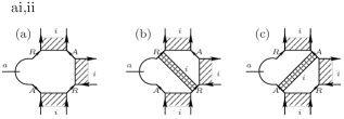
Figure 14: Diagrammatic depiction of contribution from Hikami boxes placed adjacent to leads.

If a Hikami box is placed adjacent to a lead, one finds the three contributions shown in Fig. 14. Adding these we find, with the help of Eq. (136),

$$B_{aj,jj}^{\prime} = \frac{\pi^{5}\nu_{a}\nu_{j}^{4}}{M_{j}^{4}}\mbox{ tr}\left[W_{ja}W_{aj}\frac{-M_{j}^{3}\Delta_{j}}{(M_{j}+\Delta_{j})^{4}}\right]$$ (141)

$$= -\frac{\pi^{3}\nu_{j}^{3}}{16M_{j}^{3}}f_{aj}^{\prime}.$$

This is the result reported in Eq. (80) of the main text.

References

• Altshuler and Aronov (1985) B. L. Altshuler and A. G. Aronov, in Electron-Electron Interactions in Disordered Systems, edited by A. L. Efros and M. Pollak (Elsevier, Amsterdam, 1985).
• Altshuler and Simons (1995) B. L. Altshuler and B. D. Simons, in Mesoscopic Quantum Physics, edited by E. Akkermans, G. Montambaux, J.-L. Pichard, and J. Zinn-Justin (North-Holland, 1995).
• Imry (2002) Y. Imry, Introduction to mesoscopic physics (Oxford University Press, 2002).
• Anderson et al. (1979) P. W. Anderson, E. Abrahams, and T. V. Ramakrishnan, Phys. Rev. Lett. 43, 718 (1979).
• Gorkov et al. (1979) L. P. Gorkov, A. I. Larkin, and D. E. Khmelnitskii, Pis’ma Zh. Eksp. Teor. Fiz. 30, 248 (1979) [JETP Lett. 30, 228 (1979)].
• Altshuler and Aronov (1979a) B. L. Altshuler and A. G. Aronov, Zh. Eksp. Teor. Fiz. 77, 2028 (1979a).
• Aleiner et al. (1999) I. L. Aleiner, B. L. Altshuler, and M. E. Gershenson, Waves in Random Media 9, 201 (1999).
• Zala et al. (2001) G. Zala, B. N. Narozhny, and I. L. Aleiner, Phys. Rev. B 64, 214204 (2001).
• Bouchiat (1995) H. Bouchiat, in Mesoscopic Quantum Physics, edited by E. Akkermans, G. Montambaux, J.-L. Pichard, and J. Zinn-Justin (North-Holland, 1995).
• Pierre et al. (2003) F. Pierre, A. B. Gougam, A. Anthore, H. Pothier, D. Esteve, and N. O. Birge, Phys. Rev. B 68, 085413 (2003).
• (11) Apparent contradictions between theory and experiment Pothier et al. (1997); Mohanty et al. (1997) have lead to improved understanding of the role of magnetic impurities and of the sample purity required to observe the intrinsic temperature dependence caused by electron-electron interactions alone, see Refs. Pierre and Birge, 2002; Pierre et al., 2003; Huard et al., 2005 and references therein.
• Pothier et al. (1997) H. Pothier, S. Guéron, N. O. Birge, D. Esteve, and M. H. Devoret, Phys. Rev. Lett. 79, 3490 (1997).
• Mohanty et al. (1997) P. Mohanty, E. M. Q. Jariwala, and R. A. Webb, Phys. Rev. Lett. 78, 3366 (1997).
• Pierre and Birge (2002) F. Pierre and N. O. Birge, Phys. Rev. Lett. 89, 206804 (2002).
• Huard et al. (2005) B. Huard, A. Anthore, N. O. Birge, H. Pothier, and D. Esteve, Phys. Rev. Lett. 95, 036802 (2005).
• Marcus et al. (1997) C. M. Marcus, S. R. Patel, A. G. Huibers, S. M. Cronenwett, M. Switkes, I. H. Chan, R. M. Clarke, J. A. Folk, S. F. Godijn, K. Campman et al., Chaos, Solitons & Fractals 8, 1261 (1997).
• Sivan et al. (1994) U. Sivan, Y. Imry, and A. G. Aronov, Europhys. Lett. 28, 115 (1994).
• Ya. M. Blanter (1996) Ya. M. Blanter, Phys. Rev. B 54, 12807 (1996).
• (19) Equation (1) was originally proposed as the dephasing rate in closed quantum dots, see Ref. Sivan et al., 1994. It has later been corrected to include effects following from the discrete spectrum. For open quantum dots the spectrum is continuous and the original estimate is expected to be applicable.
• Marcus et al. (1993) C. M. Marcus, R. M. Westervelt, P. F. Hopkins, and A. C. Gossard, Phys. Rev. B 48, 2460 (1993).
• Clarke et al. (1995) R. M. Clarke, I. H. Chan, C. M. Marcus, C. I. Duruöz, J. S. Harris, K. Campman, and A. C. Gossard, Phys. Rev. B 52, 2656 (1995).
• Baranger and Mello (1995) H. U. Baranger and P. A. Mello, Phys. Rev. B 51, 4703 (1995).
• Brouwer (1995) P. W. Brouwer, Phys. Rev. B 51, 16878 (1995).
• Beenakker and Michaelis (2005) C. W. J. Beenakker and B. Michaelis, J. Phys. A: Math. Gen. 38, 10639 (2005).
• Forster et al. (2007) H. Forster, P. Samuelsson, S. Pilgram, and M. Buttiker, Phys. Rev. B 75, 035340 (2007).
• Nazarov (1994) Yu. V. Nazarov, Physical Review Letters 73, 1420 (1994).
• (27) For quantum dots in semiconductor heterostructures that are defined by metal gates, the contact conductances are set independently by gate voltages. Each contact conductance can be measured by choosing gate voltages such that all other contacts are open, whereas the capacitances can be measured by closing off all contacts so that the device is in the Coulomb blockade regime. See e.g., Ref. Livermore et al., 1996, where this procedure is used for a double quantum dot.
• Livermore et al. (1996) C. Livermore, C. H. Crouch, R. M. Westervelt, K. L. Campman, and A. C. Gossard, Science 274, 1332 (1996).
• Beloborodov et al. (2003a) I. S. Beloborodov, K. B. Efetov, A. V. Lopatin, and V. M. Vinokur, Phys. Rev. Lett. 91, 246801 (2003a).
• Golubev and Zaikin (2004a) D. S. Golubev and A. D. Zaikin, Phys. Rev. B 70, 165423 (2004a).
• Brouwer and Kupferschmidt (2007) P. W. Brouwer and J. N. Kupferschmidt, arXiv:0712.1055 (2007).
• Devoret et al. (1990) M. H. Devoret, D. Esteve, H. Grabert, G.-L. Ingold, H. Pothier, and C. Urbina, Phys. Rev. Lett. 64, 1824 (1990).
• Girvin et al. (1990) S. M. Girvin, L. I. Glazman, M. Jonson, D. R. Penn, and M. D. Stiles, Phys. Rev. Lett. 64, 3183 (1990).
• Yu. V. Nazarov (1989) Yu. V. Nazarov, Pis’ma Zh. Eksp. Teor. Fiz. 49, 105 (1989) [JETP Lett. 49, 126 (1989)].
• Flensberg (1993) K. Flensberg, Phys. Rev. B 48, 11156 (1993).
• Furusaki and Matveev (1995a) A. Furusaki and K. A. Matveev, Phys. Rev. Lett. 75, 709 (1995a).
• Furusaki and Matveev (1995b) A. Furusaki and K. A. Matveev, Phys. Rev. B 52, 16676 (1995b).
• Golubev and Zaikin (2001) D. S. Golubev and A. D. Zaikin, Phys. Rev. Lett. 86, 4887 (2001).
• Levy Yeyati et al. (2001) A. Levy Yeyati, A. Martin-Rodero, D. Esteve, and C. Urbina, Phys. Rev. Lett. 87, 046802 (2001).
• Kindermann and Yu. V. Nazarov (2003) M. Kindermann and Yu. V. Nazarov, Phys. Rev. Lett. 91, 136802 (2003).
• Golubev and Zaikin (2004b) D. S. Golubev and A. D. Zaikin, Phys. Rev. B 69, 075318 (2004b).
• Bagrets and Yu. V. Nazarov (2005) D. A. Bagrets and Yu. V. Nazarov, Phys. Rev. Lett. 94, 056801 (2005).
• Brouwer et al. (2005a) P. W. Brouwer, A. Lamacraft, and K. Flensberg, Phys. Rev. Lett. 94, 136801 (2005a).
• Brouwer et al. (2005b) P. W. Brouwer, A. Lamacraft, and K. Flensberg, Phys. Rev. B 72, 075316 (2005b).
• Altshuler and Aronov (1979b) B. L. Altshuler and A. G. Aronov, Solid State Commun. 30, 115 (1979b).
• Ahmadian et al. (2005) Y. Ahmadian, G. Catelani, and I. L. Aleiner, Phys. Rev. B 72, 245315 (2005).
• Aleiner et al. (2002) I. L. Aleiner, P. W. Brouwer, and L. I. Glazman, Phys. Rep. 358, 309 (2002).
• Baranger and Mello (1994) H. U. Baranger and P. A. Mello, Phys. Rev. Lett. 73, 142 (1994).
• Jalabert et al. (1994) R. A. Jalabert, J.-L. Pichard, and C. W. J. Beenakker, Europhys. Lett 27, 255 (1994).
• Efetov (1995) K. B. Efetov, Phys. Rev. Lett. 74, 2299 (1995).
• Argaman (1995) N. Argaman, Phys. Rev. Lett. 75, 2750 (1995).
• Argaman (1996) N. Argaman, Phys. Rev. B 53, 7035 (1996).
• Aleiner and Larkin (1996) I. L. Aleiner and A. I. Larkin, Phys. Rev. B 54, 14423 (1996).
• Brouwer and Beenakker (1996) P. W. Brouwer and C. W. J. Beenakker, J. Math. Phys. 37, 4904 (1996).
• Vavilov and Aleiner (1999) M. G. Vavilov and I. L. Aleiner, Phys. Rev. B 60, R16311 (1999).
• Richter and Sieber (2002) K. Richter and M. Sieber, Phys. Rev. Lett. 89, 206801 (2002).
• Whitney (2007) R. S. Whitney, Phys. Rev. B 75, 235404 (2007).
• Seelig and Büttiker (2001) G. Seelig and M. Büttiker, Phys. Rev. B 64, 245313 (2001).
• Seelig et al. (2003) G. Seelig, S. Pilgram, and M. Buttiker, Turk. J. Phys. 27, 331 (2003).
• (60) Y. Takane, J. Phys. Soc. Jpn. 67, 3003 (1998), claims that the uniform mode can suppress weak localization, but his calculation fails to take into account that both trajectories involved in the weak localization correction experience the same phase shift from the uniform interaction mode.
• Campagnano and Nazarov (2006) G. Campagnano and Yu. V. Nazarov, Phys. Rev. B 74, 125307 (2006).
• Golubev and Zaikin (2006) D. S. Golubev and A. D. Zaikin, Phys. Rev. B 74, 245329 (2006).
• Golubev and Zaikin (2007) D. S. Golubev and A. D. Zaikin, arXiv:cond-mat/0702207 (2007).
• Texier and Montambaux (2004) C. Texier and G. Montambaux, Phys. Rev. Lett. 92, 186801 (2004).
• Texier and Montambaux (2007) C. Texier and G. Montambaux, Phys. Rev. B 76, 094202 (2007).
• Beloborodov et al. (2007) I. S. Beloborodov, A. V. Lopatin, V. M. Vinokur, and K. B. Efetov, Rev. Mod. Phys. 79, 469 (2007).
• Beloborodov et al. (2001) I. S. Beloborodov, K. B. Efetov, A. Altland, and F. W. J. Hekking, Physical Review B 63, 115109 (2001).
• Beloborodov et al. (2003b) I. S. Beloborodov, A. V. Andreev, and A. I. Larkin, Phys. Rev. B 68, 024204 (2003b).
• Efetov and Tschersich (2003) K. B. Efetov and A. Tschersich, Phys. Rev. B 67, 174205 (2003).
• Beloborodov et al. (2004) I. S. Beloborodov, A. V. Lopatin, and V. M. Vinokur, Phys. Rev. B 70 205120 (2004).
• Blanter et al. (2006) Y. M. Blanter, V. M. Vinokur, and L. I. Glazman, Phys. Rev. B 73, 165322 (2006).
• Altshuler et al. (1982) B. L. Altshuler, A. G. Aronov, and D. E. Khmelnitskii, J. Phys. C 15, 7367 (1982).
• Landau and Lifshitz (1958) L. D. Landau and E. M. Lifshitz, Statistical Physics, vol. 5 of Course of Theoretical Physics (Pergamon, London, 1958).
• Zee (2003) A. Zee, Quantum Field Theory in a nutshell (Princeton University Press, 2003).
• Melsen et al. (1996) J. A. Melsen, P. W. Brouwer, K. M. Frahm, and C. W. J. Beenakker, Europhys. Lett. 35, 7 (1996).
• Clerk and Ambegaokar (2000) A. A. Clerk and V. Ambegaokar, Phys. Rev. B 61, 9109 (2000).
• Vavilov et al. (2001) M. G. Vavilov, V. Ambegaokar, and I. L. Aleiner, Phys. Rev. B 63, 195313 (2001).
• Abrikosov et al. (1963) A. Abrikosov, L. P. Gorkov, and I. E. Dzyaloshinski, Methods of quantum field theory in statistical physics (Prentice-Hall, 1963).
• Hikami (1981) S. Hikami, Physical Review B 24, 2671 (1981).
• Golubev and Zaikin (1998) D. S. Golubev and A. D. Zaikin, Phys. Rev. Lett. 81, 1074 (1998).
• von Delft (2005) J. von Delft, Int. J. Mod. Phys. B 22, 727 (2008); arXiv:cond-mat/0510563 (2005).
• Waugh et al. (1995) F. R. Waugh, M. J. Berry, D. J. Mar, R. M. Westervelt, K. L. Campman, and A. C. Gossard, Phys. Rev. Lett. 75, 705 (1995).
• Oosterkamp et al. (1998) T. H. Oosterkamp, S. F. Godijn, M. J. Uilenreef, Yu. V. Nazarov, N. C. van der Vaart, and L. P. Kouwenhoven, Phys. Rev. Lett. 80, 4951 (1998).
• Holleitner et al. (2001) A. W. Holleitner, C. R. Decker, H. Qin, K. Eberl, and R. H. Blick, Phys. Rev. Lett. 87, 256802 (2001).
• van der Wiel et al. (2003) W. G. van der Wiel, S. De Franceschi, J. M. Elzerman, T. Fujisawa, S. Tarucha, and L. P. Kouwenhoven, Rev. Mod. Phys. 75, 1 (2003).