Superconductivity in one dimension

Abstract

Superconducting properties of metallic nanowires can be entirely different from those of bulk superconductors because of the dominating role played by thermal and quantum fluctuations of the order parameter. For superconducting wires with diameters below $\sim 50$ nm quantum phase slippage is an important process which can yield a non-vanishing wire resistance down to very low temperatures. Further decrease of the wire diameter, for typical material parameters down to $\sim 10$ nm, results in proliferation of quantum phase slips causing a sharp crossover from superconducting to normal behavior even at $T=0$. A number of interesting phenomena associated both with quantum phase slips and with the parity effect occur in superconducting nanorings. We review recent theoretical and experimental activities in the field and demonstrate dramatic progress in understanding of the phenomenon of superconductivity in quasi-one-dimensional nanostructures.

I Introduction

The phenomenon of superconductivity was discovered Kamerlingh-Onnes as a sudden drop of resistance to immeasurably small value. With the development of the topic it was realized that the superconducting phase transition is frequently not at all ”sudden” and the measured dependence of the sample resistance $R(T)$ in the vicinity of the critical temperature $T_{C}$ may have a finite width. One possible reason for this behavior – and frequently the dominating factor – is the sample inhomogeneity, i.e. the sample might simply consist of regions with different local critical temperatures. However, with improving fabrication technologies it became clear that even for highly homogeneous samples the superconducting phase transition may remain broadened. This effect is usually very small in bulk samples and becomes more pronounced in systems with reduced dimensions. A fundamental physical reason behind such smearing of the transition is superconducting fluctuations.

An important role of fluctuations in reduced dimension is well known. Above $T_{C}$ such fluctuations yield an enhanced conductivity of metallic systems almt ; Maki ; Thomson ; LV . For instance, the so-called Aslamazov-Larkin fluctuation correction to conductivity $\delta\sigma_{AL}\sim(T-T_{C})^{-(2-D/2)}$ becomes large in the vicinity of $T_{C}$ and this effect increases with decreasing dimensionality $D$. Below $T_{C}$ – according to the general theorem HMW ; Mermin 1966 – fluctuations should destroy the long-range order in low dimensional superconductors. Thus, it could naively be concluded that low dimensional conductors cannot exhibit superconducting properties because of strong phase fluctuation effects.

This conclusion, however, turns out to be somewhat premature. For instance, 2D structures undergo Berezinskii-Kosterlitz-Thouless (BKT) phase transition b ; kt ; Kosterlilz 1974 as a result of which the decay of correlations in space changes from exponential at high enough $T$ to power law at low temperatures. This result implies that at low $T$ long range phase coherence essentially survives in samples of a finite size and, hence, 2D films can well exhibit superconducting properties.

Can superconductivity survive also in (quasi)-1D systems or do fluctuations suppress phase coherence thus disrupting any supercurrent? The answer to this question would clearly be of both fundamental interest and practical importance. On one hand, investigations of this subject definitely help to encover novel physics and shed more light on the crucial role of superconducting fluctuations in 1D wires. On the other hand, rapidly progressing miniaturization of nanodevices opens new horizons for applications of superconducting nanocircuits and requires better understanding of fundamental limitations for the phenomenon of superconductivity in reduced dimension. A detailed review of the present status of this field is the main purpose of this paper.

It was first pointed out by Little Little that quasi-one-dimensional wires made of a superconducting material can acquire a finite resistance below $T_{C}$ of a bulk material due to the mechanism of thermally activated phase slips (TAPS). Within the Ginzburg-Landau theory one can describe a superconducting wire by means of a complex order parameter $\Psi(x)=|\Psi(x)|e^{i\varphi(x)}$. Thermal fluctuations cause deviations of both the modulus and the phase of this order parameter from their equilibrium values. A non-trivial fluctuation corresponds to temporal suppression of $|\Psi(x)|$ down to zero in some point (e.g., $x=0$) inside the wire, see Fig. 1. As soon as the modulus of the order parameter $|\Psi(0)|$ vanishes the phase $\varphi(0)$ becomes unrestricted and can jump by the value $2\pi n$, where $n$ is any integer number. After this process the modulus $|\Psi(0)|$ gets restored, the phase becomes single valued again and the system returns to its initial state accumulating the net phase shift $2\pi n$. Provided such phase slip events are sufficiently rare, one can restrict $n$ by $n=\pm 1$ and totally disregard fluctuations with $|n|\geq 2$.

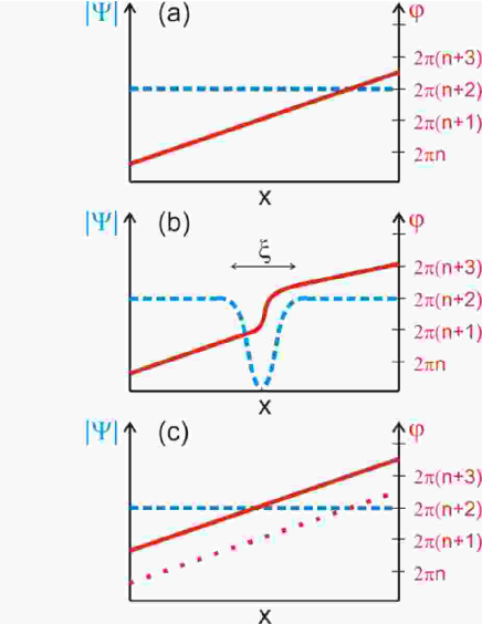
Figure 1: Schematics of the phase slip process. Spatial variation of the amplitude of the order parameter $|\Psi|$ (left axis, dashed line) and phase $\varphi$ (right axis solid line) at various moments of time: (a) before, (b) during  and (c) after the phase slippage.

According to the Josephson relation $V=\hbar\dot{\varphi}/2e$ each such phase slip event causes a nonzero voltage drop $V$ across the wire. In the absence of any bias current the net average numbers of ”positive” ($n=+1$) and ”negative” ($n=-1$) phase slips are equal, thus the net voltage drop remains zero. Applying the current $I\propto\mid\Psi\mid^{2}\nabla\varphi$ one creates nonzero phase gradient along the wire and makes ”positive” phase slips more likely than ”negative” ones. Hence, the net voltage drop $V$ due to TAPS differs from zero, i.e. thermal fluctuations cause non-zero resistance $R=V/I$ of superconducting wires even below $T_{C}$. We would also like to emphasize that, in contrast to the so-called phase slip centers Meyer IV ; Tidecks ; ivko ; Kopnin book produced by a large current above the critical one $I>I_{C}$, here we are dealing with fluctuation-induced phase slips which can occur at arbitrarily small values $I$.

A quantitative theory of the TAPS phenomenon was first proposed by Langer and Ambegaokar la and then completed by McCumber and Halperin mh . This LAMH theory predicts that the TAPS creation rate and, hence, resistance of a superconducting wire $R$ below $T_{C}$ are determined by the activation exponent

$$R(T)\propto\exp(-U/T),\;\;\;\;\;\;\;U\sim\frac{N_{0}\Delta_{0}^{2}(T)}{2}s\xi(T),$$ (1)

where $U(T)$ is the effective potential barrier for TAPS proportional to the superconducting condensation energy ($N_{0}$ is the metallic density of states at the Fermi energy and $\Delta_{0}(T)$ is the BCS order parameter) for a part of the wire of a volume $s\xi$ where superconductivity is destroyed by thermal fluctuations ($s$ is the wire cross section and $\xi(T)$ is the superconducting coherence length). At temperatures very close to $T_{C}$ eq. (1) yields appreciable resistivity which was indeed detected experimentally Webb R(T) in Sn whiskers ; Tinkham R(T) in Sn whiskers . Close to $T_{C}$ the experimental results fully confirm the activation behavior of $R(T)$ expected from eq. (1). However, as the temperature is lowered further below $T_{C}$ the number of TAPS inside the wire decreases exponentially and no measurable wire resistance is predicted by the LAMH theory la ; mh except in the immediate vicinity of the critical temperature.

Experiments Webb R(T) in Sn whiskers ; Tinkham R(T) in Sn whiskers were done on small whiskers of typical diameters $\sim 0.5$ $\mu$m. Recent progress in nanolithographic technique allowed to fabricate samples with much smaller diameters down to – and even below – 10 nm. In such systems one can consider a possibility for phase slips to occur not only due to thermal, but also due to quantum fluctuations of the superconducting order parameter. The physical picture of quantum phase slippage is qualitatively similar to that of TAPS (see Fig. 1) except the order parameter $|\Psi(x)|$ gets virtually suppressed due the process of quantum tunneling.

Following the standard quantum mechanical arguments one can expect that the probability of such tunneling process should be controlled by the exponent $\sim\exp(-U/\hbar\omega_{0})$, i.e. instead of temperature in the activation exponent (1) one should just substitute $\hbar\omega_{0}$, where $\omega_{0}$ is an effective attempt frequency. This is because the order parameter field $\Psi(x)$ now tunnels under the barrier $U$ rather than overcomes it by thermal activation. Since such tunneling process should obviously persist down to $T=0$ one arrives at a fundamentally important conclusion that in nanowires superconductivity can be destroyed by quantum fluctuations at any temperature including $T=0$. Accordingly, such nanowires should demonstrate a non-vanishing resistivity down to zero temperature. Assuming that $\hbar\omega_{0}\sim\Delta_{0}(T)$ one would expect that at $\Delta_{0}(T)\lesssim T<T_{C}$ the TAPS dependence (1) applies while at lower $T\lesssim\Delta_{0}(T)$ quantum phase slips (QPS) take over, eventually leading to saturation of the temperature dependence $R(T)$ to a non-zero value in the limit $T\ll\Delta_{0}$.

This behavior was indeed observed: Giordano Giordano QPS PRL 1988 performed experiments which clearly demonstrated a notable resistivity of ultra-thin superconducting wires far below $T_{C}$. These observations could not be adequately interpreted within the TAPS theory and were attributed to QPS. Later other groups also reported noticeable deviations from the LAMH theory in thin (quasi-)1D wires. These experiments will be discussed in Chapter 6.

It should be noted, however, that despite these developments the idea that in realistic samples superconductivity can be destroyed by quantum fluctuations was initially received with a large portion of scepticism. On one hand, this was due to a number of unsuccessful attempts to experimentally observe the QPS phenomenon. On the other hand, some early theoretical efforts have led to the results strongly underestimating the actual QPS rate. Also, unambiguous interpretation of the observations Giordano QPS PRL 1988 in terms of QPS was questioned because of possible granularity of the samples used in those experiments. If that was indeed the case, QPS could easily be created inside weak links connecting neighboring grains. Also in this case superconducting fluctuations play a very important role sz however – in contrast to the case of uniform wires – the superconducting order parameter needs not to be destroyed during a QPS event.

First attempts to theoretically analyze the QPS effects sm ; Duan ; Chang – as well as a number of later studies – were based on the so-called time-dependent Ginzburg-Landau (TDGL) equations. Unfortunately the TDGL approach is by far insufficient for the problem in question for a number of reasons: (i) A trivial reason is that the Ginzburg-Landau (GL) expansion applies only at temperatures close to $T_{C}$ whereas in order to describe QPS one usually needs to go to lower temperatures down to $T\to 0$. (ii) More importantly, also at $T_{C}-T\ll T_{C}$ TDGL equation remains applicable only in a special limit of gapless superconductors, while it fails in a general situation considered here. (iii) TDGL approach does not account for dissipation effects due to quasiparticles inside the QPS core (in certain cases also outside this core) which are expected to reduce the probability of QPS events similarly to the standard problem of quantum tunneling with dissipation cl ; cl1 ; weiss . (iv) TDGL approach is not fully adequate to properly describe excitation of electromagnetic modes around the wire during a QPS event (this effect turns out to be particularly important for sufficiently long wires). Thus, TDGL-based description of QPS effects simply cannot be trusted, and a much more elaborate theory is highly desirable in this situation.

A microscopic theory of QPS processes in superconducting nanowires was developed ZGOZ ; ZGOZ2 ; GZ01 with the aid of the imaginary time effective action technique GZ01 ; ogzb . This theory remains applicable down to $T=0$ and properly accounts for non-equilibrium, dissipative and electromagnetic effects during a QPS event. One of the main conclusions of this theory is that in sufficiently dirty superconducting nanowires with diameters in the 10 nm range QPS probability can already be large enough to yield experimentally observable phenomena. Also, further interesting effects including quantum phase transitions caused by interactions between quantum phase slips were predicted ZGOZ ; ZGOZ2 .

An important parameter of this theory is the QPS fugacity

$$y\sim S_{\mathrm{core}}\exp(-S_{\mathrm{core}}),\quad S_{\mathrm{core}}\sim g_{\xi},$$

where $g_{\xi}$ is the dimensionless conductance of the wire segment of length $\xi$. Provided $g_{\xi}$ is very large, typically $g_{\xi}\gtrsim 100$, the fugacity $y$ remains vanishingly small, QPS events are very rare and in many cases can be totally neglected. In such case the standard BCS mean field description should apply and a finite (though possibly sufficiently long) wire remains essentially superconducting outside an immediate vicinity of $T_{C}$. For smaller $g_{\xi}\lesssim 10\div 20$ QPS effects already become important down to $T\to 0$. Finally, at even smaller $g_{\xi}\sim 1$ strong fluctuations should wipe out superconductivity everywhere in the wire. We also point out that in the case of nanowires considered here the parameter $g_{\xi}$ is related to the well known Ginzburg number as $Gi_{\mathrm{1D}}\sim 1/g_{\xi}^{2/3}$, i.e. the condition $g_{\xi}\sim 1$ also implies that the fluctuation region becomes of order $T_{C}$.

Another important parameter is the ratio between the (”superconducting”) quantum resistance unit $R_{q}=\pi\hbar/2e^{2}=6.453$ k$\Omega$ and the wire impedance $Z_{w}=\sqrt{\tilde{L}/C}$:

$$\mu=R_{q}/2Z_{w},$$

where $C$ is the wire capacitance per unit length, $\tilde{L}=4\pi\lambda_{L}^{2}/s$ is the wire kinetic inductance and $\lambda_{L}$ is the London penetration depth. Provided this parameter becomes of order one, $\mu\sim 1$, superconductivity in sufficiently long wires gets fully suppressed due to intensive fluctuations of the phase $\varphi$ of the superconducting order parameter. We note that both $g_{\xi}$ and $\mu$ scale with the wire cross section $s$ respectively as $g_{\xi}\propto s$ and $\mu\propto\sqrt{s}$. It follows immediately that with decreasing the cross section below a certain value the wire inevitably looses intrinsic superconducting properties due to strong fluctuation effects. For generic parameters both conditions $g_{\xi}\sim 1\div 10$ and $\mu\sim 1$ are typically met for wire diameters in the range $\sqrt{s}\lesssim 10$ nm.

A number of recent experimental observations are clearly consistent with the above theoretical conclusions. Perhaps the first unambiguous evidence for QPS effects in quasi-1D wires was reported by Bezryadin, Lau and Tinkham BT who fabricated sufficiently uniform superconducting wires with thicknesses down to $3\div 5$ nm and observed that several samples showed no signs of superconductivity even at temperatures well below the bulk critical temperature. Those results were later confirmed and substantially extended by different experimental groups. At present there exists an overwhelming experimental evidence for QPS effects in superconducting nanowires fabricated to be sufficiently uniform and homogeneous. Below we will analyze the main experimental results and compare them with theoretical predictions.

Yet another interesting issue is related to persistent currents (PC) in superconducting nanorings. It was demonstrated MLG that QPS effects can significantly modify PC in such systems and even lead to exponential suppression of supercurrent for sufficiently large ring perimeters. Another important factor that can substantially affect PC in isolated superconducting nanorings at low $T$ is the electron parity number. Of particular interest is the behavior of rings with odd number of electrons which can develop spontaneous supercurrent in the ground state without any externally applied magnetic flux SZ .

The structure of our Review is as follows. A theory of superconducting fluctuations in nanowires will be addressed in Chapters 2-5. In Chapter 2 we discuss a general derivation of the real time effective action of a superconductor suitable for further investigations of fluctuation effects at temperatures below $T_{C}$. We also formulate the Langevin equations and analyze their relation to TDGL-type of equations frequently used in the literature. In Chapter 3 we adopt our general formalism to the case of superconducting nanowires and demonstrate the importance of superconducting fluctuations in such structures. In Chapter 4 we will briefly review LAMH theory of thermally activated phase slips. Quantum phase slip effects will be analyzed in details in Chapter 5. Chapter 6 is devoted to an elaborate discussion of key experiments in the field and their interpretation in terms of existing theories. In Chapter 7 we will analyze persistent currents in superconducting nanorings. Chapter 8 contains a brief summary of our main observations and conclusions. Some technical details are presented in Appendix.

II Effective action, Langevin and Ginzburg-Landau equations

II.1 General formulation

The starting point of our analysis is the formal expression for the quantum evolution operator on the Keldysh contour or the so-called Keldysh “partition function”. As usually sz , the kernel of the evolution operator ${\mathcal{J}}$ can be expressed in the form of a path integral over quantum fields defined both at the forward (below denoted by the subscript _F) and the backward (denoted by the subscript _B) branches of the Keldysh contour. We have

$${\mathcal{J}} =\int{\mathcal{D}}\psi_{F/B}^{\alpha}\,{\mathcal{D}}\bar{\psi}_{F/B}^{\alpha}{\mathcal{D}}\Delta_{F/B}\,{\mathcal{D}}V_{F/B}\,{\mathcal{D}}{\bm{A}}_{F/B}$$

$$\times\,e^{iS[\psi_{F}^{\alpha},\Delta_{F},V_{F},\bm{A}_{F}]-iS[\psi_{B}^{\alpha},\Delta_{B},V_{B},\bm{A}_{B}]},$$ (2)

Here $\psi_{F/B}^{\alpha},\bar{\psi}_{F/B}^{\alpha}$ are electron Grasmann fields, $\alpha=\uparrow,\downarrow$ is the spin index, $\Delta_{F/B}$ are superconducting complex order parameter fields (which emerge as a result of the standard Hubbard-Stratonovich decoupling of the BCS coupling term sz ), $V_{F/B}$ and ${\bm{A}}_{F/B}$ are respectively the scalar and vector potentials. The action $S$ is defined as follows

$$iS =\sum_{\alpha}\int d^{4}X\bigg{[}\bar{\psi}^{\alpha}\bigg{(}i\frac{\partial}{\partial t}+\frac{1}{2m}\left(\nabla+i\frac{e}{c}\bm{A}\right)^{2}$$

$$+\,\epsilon_{F}-U(\bm{r})+eV\bigg{)}\psi^{\alpha}-\Delta\bar{\psi}^{\uparrow}\bar{\psi}^{\downarrow}-\Delta^{*}\psi^{\downarrow}\psi^{\uparrow}\bigg{]}$$

$$+\,\int d^{4}X\left(\frac{{\bm{E}}^{2}-{\bm{H}}^{2}}{8\pi}-\frac{N_{0}|\Delta|^{2}}{\lambda}\right).$$ (3)

Here $\epsilon_{F}$ is the Fermi energy, $U({\bm{r}})$ is the disorder potential, $N_{0}$ is the density of states per unit spin at the Fermi level, and $\lambda$ is the BCS coupling constant. In our notations the electron charge is $e^{*}=-e$, i.e. we define $e>0$. Here and below we employ the notation $d^{4}X=dt\,d^{3}{\bm{r}}$.

As the above action is quadratic in the electron fields one can integrate them out exactly. After that one arrives at the path integral

$${\mathcal{J}}=\int{\mathcal{D}}\Delta_{F/B}\,{\mathcal{D}}V_{F/B}\,{\mathcal{D}}{\bm{A}}_{F/B}\;e^{iS_{\mathrm{eff}}[\Delta_{F/B},V_{F/B},{\bm{A}}_{F/B}]},$$ (4)

where the effective action reads

$$iS_{\mathrm{eff}}=i\int d^{4}X\left(\frac{{\bm{E}}^{2}-{\bm{H}}^{2}}{8\pi}-\frac{N_{0}|\Delta|^{2}}{\lambda}\right)+\,\mathrm{Tr}\,\ln\check{\mathcal{G}}^{-1}.$$ (5)

The inverse $4\times 4$ matrix Green-Keldysh function $\check{\mathcal{G}}^{-1}$ can be split into $2\times 2$ sub-blocks (indicated by a hat):

$$\check{\mathcal{G}}^{-1}=\left(\begin{array}[c]{cc}\hat{\mathcal{G}}^{-1}_{11}&-\hat{\sigma}_{z}\hat{\Delta}\\ -\hat{\sigma}_{z}\hat{\Delta}&\hat{\mathcal{G}}^{-1}_{22}\end{array}\right)$$ (8)

where

$$\hat{\mathcal{G}}^{-1}_{11} =\hat{\sigma}_{z}\left(i\frac{\partial}{\partial t}-H_{0}+\frac{i}{2}\{\nabla,\hat{\bm{v}}_{S}\}-\frac{m\hat{\bm{v}}_{S}^{2}}{2}+e\hat{\Phi}\right)$$

$$\hat{\mathcal{G}}^{-1}_{22} =\hat{\sigma}_{z}\left(i\frac{\partial}{\partial t}+H_{0}+\frac{i}{2}\{\nabla,\hat{\bm{v}}_{S}\}+\frac{m\hat{\bm{v}}_{S}^{2}}{2}-e\hat{\Phi}\right).$$ (9)

Here $H_{0}=-\nabla^{2}/2m+U(\bm{r})-\epsilon_{F}$ is the single electron Hamiltonian,

$$\hat{\bm{v}}_{S}=\frac{1}{2m}\left(\begin{array}[c]{cc}\nabla\varphi_{F}+\frac{2e}{c}{\bm{A}}_{F}&0\\ 0&\nabla\varphi_{B}+\frac{2e}{c}{\bm{A}}_{B}\end{array}\right),$$ (12)

$$\hat{\Phi}=\left(\begin{array}[c]{cc}V_{F}-\frac{\dot{\varphi}_{F}}{2e}&0\\ 0&V_{B}-\frac{\dot{\varphi}_{B}}{2e}\end{array}\right),$$ (15)

define the gauge invariant combiantions of the superconducting order parameter phase $\varphi$ and the electromagnetic potentials. The matrix $\hat{\Delta}$ is constructed analogously. It reads

$$\hat{\Delta}=\left(\begin{array}[c]{cc}\Delta_{F}&0\\ 0&\Delta_{B}\end{array}\right).$$ (18)

Note that both fields $\Delta_{F}$ and $\Delta_{B}$ are now real since we have already decoupled the phase factors $\varphi_{F/B}$ by the gauge transformation.

II.2 Perturbation theory

Although the above expression for the effective action $S_{\mathrm{eff}}$ (5) is exact it remains too complicated for practical calculations. In order to proceed let us – analogously to the derivation in the Matsubara technique ogzb ; GZ01 – restrict our analysis to quadratic fluctuations. For this purpose we split the order parameter into the BCS mean field term $\Delta_{0}$ and the fluctuating part. Performing a shift $\Delta_{F/B}\to\Delta_{0}+\Delta_{F/B}$ we re-define the order parameter field in a way to describe fluctuations by the fields $\Delta_{F/B}$. Expanding the effective action (5) in powers of $\hat{\Delta}$, $\hat{\bm{v}}_{S}$ and $\hat{\Phi}$ to the second order we obtain the action describing the quadratic fluctuations in the system

$$iS_{\mathrm{eff}}^{(2)}=iS_{1}+iS_{\Delta}+iS_{\mathrm{em}}+iS_{\varphi\Delta},$$ (19)

where

$$iS_{1} =\,\mathrm{Tr}\,\bigg{[}\hat{\sigma}_{z}\frac{i}{2}\{\nabla,\hat{v}_{S}\}(\hat{G}+\hat{\bar{G}})$$

$$+\,\hat{\sigma}_{z}e\hat{\Phi}(\hat{G}-\hat{\bar{G}})-\hat{\sigma}_{z}\hat{\Delta}(\hat{F}+\hat{\bar{F}})\bigg{]}$$ (20)

defines the first order (in $\hat{\Phi},\hat{\bm{v}}_{S},\hat{\Delta}$) contribution to the action,

$$iS_{\Delta}=-i\frac{N_{0}}{\lambda}\int d^{4}X\,\big{(}|\Delta_{0}+\Delta_{F}|^{2}-|\Delta_{0}+\Delta_{B}|^{2}\big{)}$$

$$-\,\frac{1}{2}\,\mathrm{Tr}\,\left\{(\hat{F}\hat{\sigma}_{z}\hat{\Delta})^{2}+(\hat{\bar{F}}\hat{\sigma}_{z}\hat{\Delta})^{2}+2\hat{\bar{G}}\hat{\sigma}_{z}\hat{\Delta}\hat{G}\hat{\sigma}_{z}\hat{\Delta}\right\},\;\;\;\;$$ (21)

accounts for fluctuations of the absolute value of the order parameter field,

$$iS_{\mathrm{em}}=i\int d^{4}X\;\frac{\bm{E}_{F}^{2}-\bm{E}_{B}^{2}-\bm{H}_{F}^{2}+\bm{H}_{B}^{2}}{8\pi}$$

$$-\,\frac{1}{2}\,\mathrm{Tr}\,\bigg{\{}m\hat{\bm{v}}_{S}^{2}(\hat{G}-\hat{\bar{G}})+\left[\hat{\sigma}_{z}\left(\frac{i}{2}\{\nabla,\hat{\bm{v}}_{S}\}+e\hat{\Phi}\right)\hat{G}\right]^{2}$$

$$+\hat{\sigma}_{z}\left(\frac{i}{2}\{\nabla,\hat{\bm{v}}_{S}\}+e\hat{\Phi}\right)\hat{F}\hat{\sigma}_{z}\left(\frac{i}{2}\{\nabla,\hat{\bm{v}}_{S}\}-e\hat{\Phi}\right)\hat{\bar{F}}$$

$$+\,\left[\hat{\sigma}_{z}\left(\frac{i}{2}\{\nabla,\hat{\bm{v}}_{S}\}-e\hat{\Phi}\right)\hat{\bar{G}}\right]^{2}\bigg{\}}$$ (22)

describes electromagnetic fields and their coupling to the phase of the order parameter field and

$$iS_{\varphi\Delta}=\,\mathrm{Tr}\,\bigg{\{}\hat{\sigma}_{z}\left(\frac{i}{2}\{\nabla,\hat{\bm{v}}_{S}\}+e\hat{\Phi}\right)\hat{F}\hat{\sigma}_{z}\hat{\Delta}\hat{G}$$

$$+\,\hat{\sigma}_{z}\left(\frac{i}{2}\{\nabla,\hat{\bm{v}}_{S}\}+e\hat{\Phi}\right)\hat{G}\hat{\sigma}_{z}\hat{\Delta}\hat{\bar{F}}$$

$$+\,\hat{\sigma}_{z}\left(\frac{i}{2}\{\nabla,\hat{\bm{v}}_{S}\}-e\hat{\Phi}\right)\hat{\bar{G}}\hat{\sigma}_{z}\hat{\Delta}\hat{F}$$

$$+\,\hat{\sigma}_{z}\left(\frac{i}{2}\{\nabla,\hat{\bm{v}}_{S}\}-e\hat{\Phi}\right)\hat{\bar{F}}\hat{\sigma}_{z}\hat{\Delta}\hat{\bar{G}}\bigg{\}}.$$ (23)

is responsible for coupling of electromagnetic and phase fluctuations to the absolute value of the order parameter field.

All the above contributions to the action are expressed in terms of equilibrium non-perturbed normal and anomalous $2\times 2$ Green-Keldysh matrices which enter as sub-blocks $\hat{G},\hat{F},\hat{\bar{G}},\hat{\bar{F}}$ into the $4\times 4$ matrix

$$\check{\mathcal{G}}_{0}=\left(\begin{array}[c]{cc}\hat{G}&\hat{F}\\ \hat{\bar{F}}&\hat{\bar{G}}\end{array}\right),$$ (26)

obtained by inverting the expression (8) at $\hat{\Phi}=0$, $\hat{\bm{A}}=0$ and $\Delta_{F}=\Delta_{B}=\Delta_{0}$. The formal expressions for the sub-blocks $\hat{G},\hat{F},\hat{\bar{G}},\hat{\bar{F}}$ are defined in Appendix A.1.

One can demonstrate that the matrix Green-Keldysh functions satisfy the Ward identities (237) and (238) specified in Appendix A.2. Making use of eq. (237) we can rewrite the first order contribution to the action in the form

$$iS_{1} =-\,\mathrm{Tr}\,\left[\hat{\sigma}_{z}\hat{\Delta}(\hat{F}+\hat{\bar{F}})\right]+i\Delta_{0}\,\mathrm{Tr}\,\left[\hat{\sigma}_{z}\hat{\varphi}(\hat{F}-\hat{\bar{F}})\right]$$

$$+\,\frac{ie}{2mc}\,\mathrm{Tr}\,\left[\hat{\sigma}_{z}\{\nabla,\hat{\bm{A}}\}(\hat{G}+\hat{\bar{G}})\right]+e\,\mathrm{Tr}\,\left[\hat{\sigma}_{z}\hat{V}(\hat{G}-\hat{\bar{G}})\right].$$

Observing that $\hat{F}=\hat{\bar{F}}$ and introducing the current $\bm{j}_{0}$ and the charge density $\rho_{0}$ in the non-perturbed state we further transform the action $iS_{1}$ and get

$$iS_{1} = -2\,\mathrm{Tr}\,\left[\hat{\sigma}_{z}\hat{\Delta}\hat{F}\right]-\frac{i}{c}\int d^{4}X\,{\bm{j}}_{0}({\bm{A}}_{F}-{\bm{A}}_{B})$$ (27)

$$-\,i\int d^{4}X\,\rho_{0}(V_{F}-V_{B}).$$

In addition, assuming the non-perturbed system state to be in thermodynamic equlibrium, we set both the current and the charge density equal zero. Then we obtain

$$iS_{1}=-2\,\mathrm{Tr}\,\left[\hat{\sigma}_{z}\hat{\Delta}\hat{F}\right].$$ (28)

Finally, we assume that the equilibrium value of the order parameter $\Delta_{0}(T)$ satisfies the standard BCS gap equation

$$\frac{1}{\lambda}=\int_{0}^{\omega_{D}}d\xi_{p}\frac{\tanh\frac{\sqrt{\xi_{p}^{2}+\Delta_{0}^{2}}}{2T}}{\sqrt{\xi_{p}^{2}+\Delta_{0}^{2}}},$$ (29)

where $\omega_{D}$ is the Debye frequency. In this case $iS_{1}$ is cancelled by the first order contribution coming from $iS_{\Delta}$ and the action does not contain the first order terms in $\delta\hat{\Delta}$ any more.

The Ward identities (237) and (238) also allow one to transform the contribution $iS_{\mathrm{em}}$ (22) and cast it to the form

$$iS_{\mathrm{em}}=iS_{J}+iS_{L}+iS_{D},$$

where the terms $iS_{J}$, $iS_{L}$ and $iS_{D}$ define the terms of a different physical origin which we will identify respectively as Josephson, London and Drude contributions to the effective action. They read

$$iS_{J}=2e^{2}\,\mathrm{Tr}\,\left[\hat{\sigma}_{z}\hat{\Phi}\hat{F}\hat{\sigma}_{z}\hat{\Phi}\hat{\bar{F}}\right],$$ (30)

$$iS_{L} = -i\int d^{4}X\;\frac{\bm{H}_{F}^{2}-\bm{H}_{B}^{2}}{8\pi}$$ (31)

$$+\,2\,\mathrm{Tr}\,\left[\hat{\sigma}_{z}\{\nabla,\hat{\bm{v}}_{S}\}\hat{F}\hat{\sigma}_{z}\{\nabla,\hat{\bm{v}}_{S}\}\hat{\bar{F}}\right],$$

$$iS_{D}=i\int d^{4}X\;\frac{\bm{E}_{F}^{2}-\bm{E}_{B}^{2}}{8\pi}$$

$$+\,\frac{1}{2}\,\mathrm{Tr}\,\bigg{[}\left(\hat{\sigma}_{z}\{\nabla,\hat{\bm{u}}\}\hat{G}\right)^{2}+\left(\hat{\sigma}_{z}\{\nabla,\hat{\bm{u}}\}\hat{\bar{G}}\right)^{2}$$

$$-\,2\hat{\sigma}_{z}\{\nabla,\hat{\bm{u}}\}\hat{F}\hat{\sigma}_{z}\{\nabla,\hat{\bm{u}}\}\hat{\bar{F}}-4m\hat{\sigma}_{z}\hat{\bm{u}}^{2}(\hat{G}-\hat{\bar{G}})\bigg{]},\;\;$$ (32)

where

$$\hat{\bm{u}}=\frac{e}{2m}\left(\int_{t_{0}}^{t}dt^{\prime}\,\nabla\hat{V}+\frac{1}{c}\hat{\bm{A}}\right).$$ (33)

At low frequencies and temperatures the Josephson contribution $iS_{J}$ can be large, thus suppressing fluctuations of the gauge invariant potential $\hat{\Phi}$. In this case one can set $\hat{\Phi}=0$ and get $\hat{\dot{\phi}}=2e\hat{V}$, which is just the well known Josephson relation between the phase and the electric potential. Note that for ultra-thin superconducting wires the Josephson relation can be violated, as it will be demonstrated below.

The London contribution $iS_{L}$ is responsible for the screening of the magnetic field penetrating inside the superconductor. Finally, the Drude contribution $iS_{D}$ remains non-zero in the normal state where it accounts for Ohmic dissipation due to flowing electric currents. Since the correction to the magnetic susceptibility in normal metals is usually small, one can ignore the vector potential in the expression for $\hat{\bm{u}}$ (33). Afterwards one can again apply the Ward identities (238) and rewrite $iS_{D}$ in the form

$$iS_{D} =i\int d^{4}X\;\frac{\bm{E}_{F}^{2}-\bm{E}_{B}^{2}}{8\pi}$$

$$-\,\frac{e^{2}}{2}\,\mathrm{Tr}\,\bigg{[}\left(\hat{\sigma}_{z}\hat{V}\hat{G}\right)^{2}+\left(\hat{\sigma}_{z}\hat{V}\hat{\bar{G}}\right)^{2}+2\hat{\sigma}_{z}\hat{V}\hat{F}\hat{\sigma}_{z}\hat{V}\hat{\bar{F}}\bigg{]}.\;\;\;\;\;$$ (34)

At last, let us consider the cross term $iS_{\varphi\Delta}$. Again applying the identity (237) we cast this term to the form similar to eq. (27):

$$iS_{\varphi\Delta} =-\,\mathrm{Tr}\,\left[\hat{\sigma}_{z}\hat{\Delta}\left(\delta\hat{F}-\delta\hat{\bar{F}}\right)\right]$$

$$-\frac{i}{c}\int d^{4}X\,\delta{\bm{j}}_{0}({\bm{A}}_{F}-{\bm{A}}_{B})-i\int d^{4}X\,\delta\rho_{0}(V_{F}-V_{B}),$$

where $\delta{\bm{j}},\delta\rho_{0}\propto\Delta_{F},\Delta_{B}$ define the first order corrections to the current and the charge density due to fluctuating order parameter fields. One can verify that in the absence of both particle-hole asymmetry and charge imbalance these corrections vanish. Likewise, in this case we have $\delta\hat{F}=\delta\hat{\bar{F}}$. Thus, we conclude that

$$iS_{\varphi\Delta}=0.$$ (35)

For clarity, we now summarize again the results derived this section. The complete expression for the effective action describing quadratic fluctuations in a superconductor reads

$$iS_{\mathrm{eff}}^{(2)}=iS_{1}+iS_{\Delta}+iS_{J}+iS_{L}+iS_{D},$$ (36)

where the terms $iS_{1}$, $iS_{\Delta}$, $iS_{J}$, $iS_{L}$ and $iS_{D}$ are defined respectively in eqs. (28), (21), (30), (31) and (34).

II.3 Gaussian fluctuations in dirty superconductors

Below we will mainly be interested in the limit of so-called dirty superconductors, i.e. we assume that the concentration of defects in the system is sufficiently high and the electron motion is diffusive. In the case of ultra-thin superconducting channels only this limit appears to be of practical interest, since usually the electron elastic mean free path $l$ does not exceed the diameter of the wire. Since we will mainly focus our attention on wires with diameters in the 10 nm range, realistic values of $l$ should be typically in the same range, i.e. we have $l\ll\xi_{0}\sim\hbar v_{F}/\Delta_{0}\sim 1$ $\mu$m and $l\ll\lambda_{L}$.

In order to account for processes with characteristic length scales exceeding the electron mean free path $l$ it will be convenient for us to perform disorder averaging directly in the effective action. To this end we substitute explicit expressions for the Green functions (229) into the effective action derived in the previous section and then apply the standard rules of averaging for the electron wave functions. In the diffusion approximation we have

$$\sum_{mn}\left\langle\delta(\xi_{n}-\xi_{1})\delta(\xi_{m}-\xi_{2})\chi_{n}(\bm{r})\chi_{n}(\bm{r}^{\prime})\chi_{m}(\bm{r}^{\prime})\chi_{m}(\bm{r})\right\rangle$$

$$=\frac{N_{0}}{\pi}\,\mathrm{Re}\,{\mathcal{D}}(\xi_{1}-\xi_{2},\bm{r},\bm{r}^{\prime}),$$

$$\sum_{mn}\left\langle\delta(\xi_{n}-\xi_{1})\delta(\xi_{m}-\xi_{2})\left(\nabla^{\alpha}_{\bm{r}_{1}}-\nabla^{\alpha}_{\bm{r}_{4}}\right)\left(\nabla^{\beta}_{\bm{r}_{3}}-\nabla^{\beta}_{\bm{r}_{2}}\right)\right.$$

$$\left.\chi_{n}(\bm{r}_{1})\chi_{n}(\bm{r}_{2})\chi_{m}(\bm{r}_{3})\chi_{m}(\bm{r}_{4})\right\rangle\big{|}_{\bm{r}_{4}=\bm{r}_{1}=\bm{r},\;\bm{r}_{3}=\bm{r}_{4}=\bm{r}^{\prime}}$$

$$=\,\frac{4m^{2}D}{\pi}\delta_{\alpha\beta}\,\mathrm{Re}\,\big{[}i(\xi_{1}-\xi_{2}){\mathcal{D}}(\xi_{1}-\xi_{2},\bm{r},\bm{r}^{\prime})\big{]}.$$ (37)

Here $D=v_{F}l/3$ is the diffusion constant and ${\mathcal{D}}(\omega,\bm{r},\bm{r}^{\prime})$ is the diffuson defined as a solution of the diffusion equation

$$\left(-i\omega-D\nabla^{2}_{\bm{r}}\right){\mathcal{D}}(\omega,\bm{r},\bm{r}^{\prime})=\delta(\bm{r}-\bm{r}^{\prime}).$$ (38)

In the following we will mainly consider spatially extended systems in which case one has

$${\mathcal{D}}(\omega,\bm{r},\bm{r}^{\prime})=\int\frac{d^{3}\bm{q}}{(2\pi)^{3}}\,\frac{e^{i\bm{q}(\bm{r}-\bm{r}^{\prime})}}{-i\omega+Dq^{2}}.$$ (39)

Employing eqs. (37) we arrive at the following expression for the effective action

$$iS_{\mathrm{eff}}^{(2)} =i\int d^{4}X\,\frac{\bm{E}^{-}\bm{E}^{+}-\bm{H}^{-}\bm{H}^{+}}{4\pi}$$

$$+\,i\int d^{4}Xd^{4}X^{\prime}\bigg{\{}\Delta^{-}(X)K_{\Delta}^{X,X^{\prime}}\Delta^{+}(X^{\prime})$$

$$+\,\Phi^{-}(X)K_{J}^{X,X^{\prime}}\Phi^{+}(X^{\prime})-{\bm{v}}_{S}^{-}(X)K_{L}^{X,X^{\prime}}{\bm{v}}_{S}^{+}(X^{\prime})$$

$$+\,{\bm{E}}^{-}(X)K_{D}^{X,X^{\prime}}{\bm{E}}^{+}(X^{\prime})\bigg{\}}$$

$$-\,\int d^{4}Xd^{4}X^{\prime}\bigg{\{}\Delta^{-}(X)\tilde{K}_{\Delta}^{X,X^{\prime}}\Delta^{-}(X^{\prime})$$

$$+\,\Phi^{-}(X)\tilde{K}_{J}^{X,X^{\prime}}\Phi^{-}(X^{\prime})-{\bm{v}}_{S}^{-}(X)\tilde{K}_{L}^{X,X^{\prime}}{\bm{v}}_{S}^{-}(X^{\prime})$$

$$+\,{\bm{E}}^{-}(X)\tilde{K}_{D}^{X,X^{\prime}}{\bm{E}}^{-}(X^{\prime})\bigg{\}},$$ (40)

where we introduced ”classical” $\Delta^{+}=(\Delta_{F}+\Delta_{B})/2$ and ”quantum” $\Delta^{-}=\Delta_{F}-\Delta_{B}$ components of the order parameter field and used analogous definitions for other fluctuating variables ${\bm{v}}_{S}^{\pm}$, $\Phi^{\pm}$ and ${\bm{E}}^{\pm}$. The four kernels $K_{j}^{X,X^{\prime}}$ ($j=\Delta,L,J,D$) are defined as follows

$$K_{j}^{X,X^{\prime}} =\int\frac{d^{4}Q}{(2\pi)^{4}}\,e^{-i\omega(t-t^{\prime})+i\bm{q}(\bm{r}-\bm{r}^{\prime})}\chi_{j}(Q),$$

$$\tilde{K}_{j}^{X,X^{\prime}} =\int\frac{d^{4}Q}{(2\pi)^{4}}\,e^{-i\omega(t-t^{\prime})+i\bm{q}(\bm{r}-\bm{r}^{\prime})}\,\frac{\mathrm{Im}\,[\chi_{j}(Q)]}{2}\coth\frac{\omega}{2T},$$ (41)

where we denote $d^{4}Q=d\omega d^{3}\bm{q}$.

Explicit expressions for the functions $\chi_{\Delta}$, $\chi_{J}$, $\chi_{L}$ and $\chi_{D}$ are rather cumbersome. They are presented in Appendix A.3 respectively in eqs. (242), (243), (244) and (245). Here we provide simple analytical expressions valid in some limiting cases.

Let us first concentrate on the low temperature limit $T\ll\Delta_{0}$. In this limit at small frequencies and wave vectors $\omega,Dq^{2}\ll\Delta_{0}$ we find

$$\chi_{\Delta} = -2N_{0}\left(1-\frac{\omega^{2}}{12\Delta_{0}^{2}}+\frac{\pi Dq^{2}}{8\Delta_{0}}\right),$$

$$\chi_{J} = 2e^{2}N_{0}\left(1+\frac{\omega^{2}}{6\Delta_{0}^{2}}-\frac{\pi Dq^{2}}{8\Delta_{0}}\right),$$

$$\chi_{L} = 2\pi m^{2}N_{0}D\Delta_{0},$$

$$\chi_{D} = \frac{e^{2}N_{0}D}{4\Delta_{0}},$$ (42)

while in the limit $|\omega|,Dq^{2}\gg\Delta_{0}(0)\equiv\pi e^{-\gamma}T_{C}$ ($\gamma\simeq 0.577$ is the Euler constant) one finds

$$\chi_{\Delta} =-2N_{0}\ln\frac{-i\omega+Dq^{2}}{\Delta_{0}(0)},$$

$$\chi_{J} =-\frac{8e^{2}N_{0}\Delta_{0}^{2}(T)}{\omega(\omega^{2}+D^{2}q^{4})}$$

$$\times\,\left[\omega\ln\frac{-i\omega+Dq^{2}}{\Delta_{0}(0)}-iDq^{2}\ln\frac{-i\omega}{2\Delta_{0}(0)}\right],$$

$$\chi_{L} =\frac{8m^{2}N_{0}D\Delta_{0}^{2}(T)}{\omega^{2}+D^{2}q^{4}}$$

$$\times\,\left[Dq^{2}\ln\frac{-i\omega+Dq^{2}}{\Delta_{0}(0)}+i\omega\ln\frac{-i\omega}{2\Delta_{0}(0)}\right],$$

$$\chi_{D} =\frac{\sigma}{-i\omega+Dq^{2}},$$ (43)

where $\sigma=2e^{2}N_{0}D$ is the normal state Drude conductivity. Here we explicitly indicated the temperature dependence of the superconducting gap $\Delta_{0}(T)$ in order to emphasize that these asymptotic expressions are valid at all temperatures rather than only in the limit $T\ll\Delta_{0}$.

Let us now consider higher temperatures $|T-T_{C}|\ll T_{C}$. At $T>T_{C}$ our general expression for $\chi_{\Delta}$ reduces to the standard result

$$\chi_{\Delta} =-2N_{0}\left[\ln\frac{T}{T_{C}}+\Psi\left(\frac{1}{2}+\frac{-i\omega+Dq^{2}}{4\pi T}\right)-\Psi\left(\frac{1}{2}\right)\right],$$ (44)

$\chi_{D}$ is again defined by the Drude formula (43), while two other $\chi$-functions vanish identically in this temperature interval, $\chi_{J}=\chi_{L}=0$. The latter observation implies that phase fluctuations remain unrestricted in this case. Hence, no Taylor expansion of the action in the phase $\varphi$ can be performed. In this case it is more convenient to undo the gauge transformation restoring the initial dependence of the action on the complex order parameter field and then to expand the action in this field. For simplicity ignoring electromagnetic fields and expanding the action to the second order in $\Delta^{\pm}$ we find

$$iS_{\mathrm{eff}}^{(2)}=\frac{i}{2}\int d^{4}Xd^{4}X^{\prime}\left\{\left(\Delta^{-}(X)\right)^{*}K_{\Delta}^{X,X^{\prime}}\Delta^{+}(X^{\prime})\right.$$

$$\left.+\,\Delta^{-}(X)K_{\Delta}^{X,X^{\prime}}\left(\Delta^{+}(X^{\prime})\right)^{*}\right\}$$

$$-\,\int d^{4}Xd^{4}X^{\prime}\left(\Delta^{-}(X)\right)^{*}\tilde{K}_{\Delta}^{X,X^{\prime}}\Delta^{-}(X^{\prime}).$$ (45)

In the limit of small frequencies and wave vectors $|\omega|,Dq^{2}\ll 2\pi T_{C}$ one recovers the standard expression

$$\chi_{\Delta}=-2N_{0}\ln\frac{T}{T_{C}}-\frac{\pi N_{0}}{4T}(-i\omega+Dq^{2}),$$ (46)

which usually serves as a starting point for the derivation of the so-called time dependent Ginzburg-Landau equation (TDGL) which we will address shortly below.

Turning to temperatures below the critical one, $T<T_{C}$, and expanding the $\chi$-functions (242)-(245) in powers of $\Delta_{0}$ we obtain

$$\chi_{\Delta} = -\frac{7\zeta(3)}{2\pi^{2}}\frac{N_{0}\Delta_{0}^{2}}{T^{2}}$$

$$-\,\frac{\pi N_{0}}{4T}(-i\omega+Dq^{2})-\frac{\pi N_{0}}{2T}\frac{\Delta_{0}^{2}}{-i\omega+Dq^{2}},$$

$$\chi_{J} = \frac{7\zeta(3)}{2\pi^{2}}\frac{e^{2}N_{0}\Delta_{0}^{2}}{T^{2}}$$

$$+\,\frac{\pi e^{2}N_{0}\Delta_{0}^{2}}{T}\left(\frac{1}{-i\omega+Dq^{2}}+\frac{\Delta_{0}^{2}}{\omega^{2}}\frac{-2i\omega+Dq^{2}}{\left(-i\omega+Dq^{2}\right)^{2}}\right),$$

$$\chi_{L} = \frac{\pi m^{2}N_{0}D\Delta_{0}^{2}}{T}\left(\frac{-2i\omega+Dq^{2}}{-i\omega+Dq^{2}}-\frac{\Delta_{0}^{2}}{\left(-i\omega+Dq^{2}\right)^{2}}\right),$$

$$\chi_{D} = \frac{2e^{2}N_{0}D}{-i\omega+Dq^{2}}\left(1-\frac{7\zeta(3)}{2\pi^{2}}\frac{\Delta_{0}^{2}}{T^{2}}\right)$$ (47)

$$-\,\frac{\pi e^{2}N_{0}D\Delta_{0}^{2}}{2T}\frac{1}{(-i\omega+Dq^{2})^{2}}.$$

These results apply for $\Delta_{0}\ll|\omega|,Dq^{2}$ and in the limit of small wave vectors and frequencies, $|\omega|,Dq^{2}\ll 2\pi T_{C}$. Here $\Delta_{0}(T)$ obeys the standard BCS self-consistency gap equation at $T\sim T_{C}$:

$$\ln\frac{T_{C}}{T}=\frac{7\zeta(3)}{8\pi^{2}}\frac{\Delta_{0}^{2}}{T^{2}}+\mathcal{O}\left(\frac{\Delta_{0}^{4}}{T^{4}}\right).$$ (48)

For $|\omega|,Dq^{2}\ll\Delta_{0}$ we obtain non-analytic expressions. For example, $\chi_{J}$ in this limit reads

$$\chi_{J}=\frac{e^{2}N_{0}\Delta_{0}}{2T}\bigg{\{}\frac{7\zeta(3)}{\pi^{2}}\frac{\Delta_{0}}{T}$$

$$+\,\frac{-i\omega}{\sqrt{\omega^{2}+D^{2}q^{4}}}\bigg{[}\ln\frac{\sqrt{\omega^{2}+D^{2}q^{4}}+Dq^{2}}{\sqrt{\omega^{2}+D^{2}q^{4}}-Dq^{2}}+\pi i\frac{\omega}{|\omega|}\bigg{]}\bigg{\}}.$$ (49)

More accurate expressions for the kernels $\chi_{\Delta}$, $\chi_{J}$ and $\chi_{L}$ valid at temeperatures close to $T_{C}$ and at any $|\omega|,Dq^{2}\ll 2\pi T_{C}$ are given in Appendix, see Eqs. (248-253). Only in the limit $|\omega|\ll Dq^{2}\ll\Delta_{0}$ those expressions match with the well known results for the coefficients of the linearized (time-independent) Ginzburg-Landau equation:

$$\chi_{\Delta}=-\frac{7\zeta(3)}{2\pi^{2}}\frac{N_{0}\Delta_{0}^{2}}{T^{2}},\;\;\chi_{J}=\frac{7\zeta(3)}{2\pi^{2}}\frac{e^{2}N_{0}\Delta_{0}^{2}}{T^{2}},\;\;$$

$$\chi_{L}=\frac{\pi m^{2}N_{0}D\Delta_{0}^{2}}{T}.$$ (50)

At frequencies $Dq^{2}\ll|\omega|\ll\Delta_{0}$ the functions $\chi_{\Delta}$ and $\chi_{J}$ turn out to be parametrically different taking much higher values:

$$\chi_{\Delta}=-\frac{\pi N_{0}\Delta_{0}}{4T},\;\;\chi_{J}=\frac{\pi e^{2}N_{0}\Delta_{0}}{4T},$$ (51)

while $\chi_{L}$ is still given by Eq. (50). The Drude susceptibility $\chi_{D}$ may be taken in the usual form (43) in both cases. Thus, already at small frequencies (well below the gap $\Delta_{0}\ll T_{C}$) microscopic results can strongly deviate from those frequently used within semi-phenomenological TDGL approach. At higher frequencies and/or wave vectors $|\omega|+Dq^{2}\gg\Delta_{0}$ this difference becomes even more pronounced, cf. eqs. (47).

One can demonstrate that these kernels are not independent and obey the following exact identity

$$\chi_{\Delta}=-\frac{\chi_{J}}{e^{2}}+\frac{\omega^{2}}{4e^{2}\Delta_{0}^{2}}\chi_{J}-\frac{q^{2}}{4m^{2}\Delta_{0}^{2}}\chi_{L},$$ (52)

which directly follows from the Ward identities (238). In addition, in the diffusive limit the kernels $\chi_{J}$ and $\chi_{L}$ are related to each other as

$$\chi_{L}(\omega,\bm{q})=\chi_{L}(\omega,0)-\frac{m^{2}D^{2}q^{2}}{e^{2}}\chi_{J}(\omega,\bm{q}).$$ (53)

This latter relation applies only for dirty superconductors.

For clarity, it is worthwhile to display the relation between the $\chi$-kernels derived here and some other quantities analyzed in the literature. For example, one can introduce the complex conductivity $\sigma(Q)$ of a superconductor MB

$$\bm{j}_{Q}=\sigma(Q)\bm{E}_{Q},$$ (54)

where $\bm{j}_{Q}$ and $\bm{E}_{Q}$ are the Fourier components of respectively the current density and the electric field. In Ref. AG the function ${\mathcal{Q}}(Q)$ was analyzed which expresses the current via the vector potential:

$$\bm{j}_{Q}=-{\mathcal{Q}}(Q)\bm{A}_{Q}.$$ (55)

Both ${\mathcal{Q}}(Q)$ and $\sigma(Q)$ are related to the kernels $\chi_{L}$ and $\chi_{D}$ as follows

$${\mathcal{Q}}(Q)=\frac{-i\omega}{c}\sigma(Q)=\frac{1}{c}\left[\frac{e^{2}}{m^{2}}\chi_{L}(Q)-\omega^{2}\chi_{D}(Q)\right].$$ (56)

II.4 Langevin equations

Let us now rewrite our results in a slightly different manner. The effective action $S^{(2)}_{\mathrm{eff}}$ can be equivalently defined by means of the following formula

$$e^{iS^{(2)}_{\mathrm{eff}}}=\left\langle e^{iS_{\xi}[\Delta^{\pm},{\bm{v}}_{S}^{\pm},\Phi^{\pm},{\bm{E}}^{\pm},{\bm{H}}^{\pm},\xi_{\Delta},\xi_{J},{\bm{\xi}}_{L}]}\right\rangle_{\xi_{j}},$$ (57)

where

$$iS_{\xi} =i\int d^{4}X\,\frac{\bm{E}^{-}\bm{E}^{+}-\bm{H}^{-}\bm{H}^{+}}{4\pi}$$

$$+\,i\int d^{4}Xd^{4}X^{\prime}\bigg{\{}\Delta^{-}(X)K_{\Delta}^{X,X^{\prime}}\Delta^{+}(X^{\prime})$$

$$+\,\Phi^{-}(X)K_{J}^{X,X^{\prime}}\Phi^{+}(X^{\prime})+{\bm{E}}^{-}(X)K_{D}^{X,X^{\prime}}{\bm{E}}^{+}(X^{\prime})$$

$$-\,\ {\bm{v}}_{S}^{-}(X)K_{L}^{X,X^{\prime}}{\bm{v}}_{S}^{+}(X^{\prime})\bigg{\}}$$

$$-\,i\int d^{4}X\,\big{[}\xi_{\Delta}\Delta^{-}+\xi_{J}\Phi^{-}+{\bm{\xi}}_{L}{\bm{v}}_{S}^{-}\big{]},$$ (58)

and averaging is performed over three different stochastic variables $\xi_{\Delta}$, $\xi_{J}$, ${\bm{\xi}}_{L}$ defined by the pair correlators

$$\langle\xi_{\Delta}(t,{\bm{r}})\xi_{\Delta}(0,0)\rangle =\int\frac{d^{4}Q}{(2\pi)^{4}}\,e^{-i\omega t+i{\bm{q}r}}\,\coth\frac{\omega}{2T}\,$$

$$\times\,\mathrm{Im}\,\big{[}\chi_{\Delta}(Q)\big{]},$$

$$\langle\xi_{J}(t,{\bm{r}})\xi_{J}(0,0)\rangle =\int\frac{d^{4}Q}{(2\pi)^{4}}\,e^{-i\omega t+i{\bm{q}r}}\,\coth\frac{\omega}{2T}\,$$

$$\times\,\mathrm{Im}\,\big{[}\chi_{J}(Q)+q^{2}\chi_{D}(Q)\big{]},$$

$$\langle\xi_{L}^{\alpha}(t,{\bm{r}})\xi_{L}^{\beta}(0,0)\rangle =\delta_{\alpha\beta}\int\frac{d^{4}Q}{(2\pi)^{4}}\,e^{-i\omega t+i{\bm{q}r}}\,\coth\frac{\omega}{2T}\,$$

$$\times\,\mathrm{Im}\,\left[-\chi_{L}(Q)+\frac{m^{2}\omega^{2}}{e^{2}}\chi_{D}(Q)\right],$$

$$\langle{\bm{\xi}}_{L}(t,{\bm{r}})\xi_{J}(0,0)\rangle =-\int\frac{d^{4}Q}{(2\pi)^{4}}\,e^{-i\omega t+i{\bm{q}r}}\,\coth\frac{\omega}{2T}\,$$

$$\times\,\frac{m\omega{\bm{q}}}{e}\,\mathrm{Im}\,\left[\chi_{D}(Q)\right].$$ (59)

All other cross correlators of the above stochastic variables are equal to zero.

The representation (57) is just the result of the standard Hubbard-Stratonovich decoupling transformation in the effective action (40). We have also used the identity

$${\bm{E}}^{-}=-\nabla V^{-}-\frac{1}{c}\frac{\partial{\bm{A}}}{\partial t}=-\nabla\Phi^{-}-\frac{m}{e}\frac{\partial{\bm{v}}_{S}}{\partial t}.$$ (60)

Let us now find the least action paths for $S_{\xi}$. Setting the variational derivatives of the action (58) with respect to quantum fields $\Delta^{-}$, $\varphi^{-}$, $V^{-}$ and ${\bm{A}}^{-}$ equal to zero we arrive at four different equations for the fields $\Delta^{+}$, $\varphi^{+}$, $V^{+}$ and ${\bm{A}}^{+}$ which provide the minimum for the action $S_{\xi}$ (58). The first equation describes fluctuations of the absolute value of the order parameter. It reads

$$\int d^{4}X^{\prime}\,K_{\Delta}^{X,X^{\prime}}\;\Delta^{+}(X^{\prime})=\xi_{\Delta}(X).$$ (61)

The second one is the continuity equation for the supercurrent. We obtain

$$\frac{\partial\rho_{S}}{\partial t}+\nabla\bm{j}_{S}=-\frac{\partial\xi_{J}}{\partial t}+\frac{e}{m}\nabla{\bm{\xi}}_{L},$$ (62)

where we introduced the superconducting density $\rho_{S}$ and the superconducting current density $\bm{j}_{S}$

$$\rho_{S} =-\int d^{4}X^{\prime}\,K_{J}^{X,X^{\prime}}\Phi^{+}(X^{\prime}),$$

$${\bm{j}}_{S} =-\frac{e}{m}\int d^{4}X^{\prime}\,K_{L}^{X,X^{\prime}}{\bm{v}}_{S}^{+}(X^{\prime}).$$ (63)

The remaining two saddle point equations take the form

$$\frac{\nabla{\bm{E}}^{+}(X)}{4\pi}+\int d^{4}X^{\prime}\,K_{D}^{X,X^{\prime}}\;\nabla{\bm{E}}^{+}(X^{\prime})-\rho_{S}(X)=\xi_{J}(X)$$ (64)

and

$$\frac{\nabla\times{\bm{H}}^{+}}{4\pi}=\frac{1}{4\pi c}\frac{\partial{\bm{E}}^{+}}{\partial t}+\frac{\bm{j}_{S}}{c}+\frac{\bm{j}_{N}}{c}-\frac{e}{m}{\bm{\xi}}_{L}.$$ (65)

Here

$${\bm{j}}_{N}=\int dX^{\prime}\,K_{D}^{X,X^{\prime}}\frac{\partial{\bm{E}}^{+}(X^{\prime})}{\partial t^{\prime}}$$ (66)

is the normal quasiparticle current.

Eqs. (61), (62), (64) and (65) together with noise correlators (59) represent the set of Langevin equations fully describing quantum dynamics of the order parameter and electromagnetic fields for dirty superconductors within the Gaussian approximation. As it is clear from our derivation, these equations remain valid provided the electron distribution function is not driven far from equilibrium. Generalization of our approach to non-equilibrium situations is also possible but will not be discussed here.

II.5 Time dependent Ginzburg-Landau equation

Now let us establish the relation between our results and the approach based on the so-called time dependent Ginzburg-Landau equation (TDGL) which is widely used to model various non-stationary effects in superconductors at temperatures close to $T_{C}$. For example, above the critical temperature this TDGL approach allows to correctly evaluate the so-called Aslamazov-Larkin fluctuation correction to the conductivity of the system. Below $T_{C}$ it enables one to describe formation of phase slip centers and the resistive state of current biased superconducting wires. Relative simplicity of the TDGL approach makes it possible to apply powerful numerical methods thus making this technique particularly appealing. In many cases the TDGL-based analysis was employed even far beyond its applicability range, e.g., in order to describe quantum phase slips in superconducting nanowires at $T\to 0$.

The TDGL equation is usually written in the following simple form LV

$$\bigg{[}\frac{\partial}{\partial t}-2ieV+\frac{1}{\tau_{GL}}-D\left(\nabla+i\frac{2e}{c}\bm{A}\right)^{2}$$

$$+\frac{7\zeta(3)}{\pi^{3}T}|\Delta|^{2}\bigg{]}\Delta=\tilde{\xi}_{\Delta},$$ (67)

where

$$\tau_{GL}=\frac{\pi}{8|T-T_{C}|}$$ (68)

is the so-called Ginzburg-Landau time and

$$\langle\tilde{\xi}_{\Delta}^{*}(t,\bm{r})\tilde{\xi}_{\Delta}(t^{\prime},\bm{r}^{\prime})\rangle=\frac{16T^{2}}{\pi N_{0}}\delta(t-t^{\prime})\delta(\bm{r}-\bm{r}^{\prime}).$$ (69)

Although this form can be justified for gapless superconductors at high concentration of magnetic impurities, in general no consistent microscopic derivation of eq. (67) was ever performed. Nevertheless, it is usually believed that eq. (67) is microscopically justified at temperatures above $T_{C}$ where the average value of the BCS order parameter is zero, $\Delta_{0}=0$. Unfortunately, our present microscopic derivation (as well as earlier imaginary time analysis GZ01 ; ogzb ) does not fully support this statement. An independent analysis based on the real-time non-linear $\sigma$-model was recently performed by Levchenko and Kamenev LK who also noticed that even at $T>T_{C}$ eq. (67) is not quite correct. These authors formulated a more accurate real-time TDGL equation in the form convenient for a comparison with eq. (67):

$$\bigg{[}\frac{\partial}{\partial t}-2ie\frac{\partial{\mathcal{K}}(X)}{\partial t}+\frac{1}{\tau_{GL}}-D\left(\nabla+i\frac{2e}{c}\bm{A}(X)\right)^{2}$$

$$+\,\frac{7\zeta(3)}{\pi^{3}T}|\Delta(X)|^{2}\bigg{]}\Delta(X)-\frac{7\zeta(3)}{\pi^{3}T}\Delta(X)\int d^{4}X^{\prime}{\mathcal{D}}(X,X^{\prime})$$

$$\times\,\left(\Delta^{*}(X^{\prime})\frac{\partial\Delta(X^{\prime})}{\partial t^{\prime}}-2ei|\Delta(X^{\prime 2}\frac{\partial{\mathcal{K}}(X^{\prime})}{\partial t^{\prime}}\right)=\tilde{\xi}_{\Delta}(X),$$ (70)

where ${\mathcal{K}}(X)=\int dX^{\prime}{\mathcal{D}(X,X^{\prime})}\big{[}V(X^{\prime})-D\nabla{\bm{A}}(X^{\prime})\big{]}$.

It is obvious that eq. (70) does not in general coincide with eq. (67). At the same time, it is satisfactory to observe that eq. (70) agrees with our results up to terms $\sim\Delta^{+},\varphi^{+}$. In order to demonstrate this fact it is necessary to identify $\Delta=(\Delta_{0}+\Delta^{+})e^{i\varphi^{+}}$ and consider terms linear in $\Delta^{+}$ and $\varphi^{+}$. In this way one arrives at our Langevin eqs. (61)-(62) with $\Delta_{0}=$const, where the functions $\chi_{\Delta}$, $\chi_{J}$, $\chi_{L}$ coincide with those given by Eq. (47) in the leading order in $\Delta_{0}$. Thus, we conclude that in the limit $\Delta_{0}\to 0$ our Langevin equations are equivalent to TDGL-type of equation LK within the order $\sim\Delta_{0}^{2}$. Some differences, however, arise for higher order terms, namely for terms $\sim\Delta_{0}^{4}$ originating from the functions $\chi_{J}$ and $\chi_{L}$ as well as for terms $\sim\Delta_{0}^{2}$ emerging from $\chi_{\Delta}$. This observation indicates that eq. (70) is still not fully justified at temperatures $T<T_{C}$.

In fact, it is not quite clear to us whether it would be of any practical importance to pursue the GL expansion up to terms $\sim\Delta^{3}$ in the TDGL-type equations. Of course, a regular expansion in powers of $\Delta^{\pm}$ can be performed in the initial effective action (5). In the order $\sim\Delta^{4}$ this expansion generates many complicated non-local (both in space and in time) terms containing the quantum field $(\Delta^{-})^{n}$ with $n$ ranging from 1 to 4. In order to recover terms $\sim\Delta^{3}$ in the TDGL equation one should disregard all terms in the action $\sim(\Delta^{-})^{n}$ with $n\geq 2$. In certain situations this approximation might be difficult to justify. In addition, the remaining terms $\sim\Delta^{3}$ are hardly tractable except in the zero frequency limit. Finally, the whole approach remains restricted to temperatures $T\sim T_{C}$. In view of all these problems it appears more appealing to perform the expansion of the effective action in superconducting fluctuations around the mean field value $\Delta_{0}$. This strategy was pursued in the bulk of this chapter. Restricting these expansion to second order terms in $\Delta^{\pm}$ we arrive at the Langevin equations (61)-(62) with $\chi_{\Delta}$, $\chi_{J}$ and $\chi_{L}$ defined in Eqs. (242-244). This approach remains applicable at all temperatures down to $T=0$ and is sufficient for practical calculations in a large number of situations.

III Thin metallic wires

We now turn to the specific case of sufficiently long and very thin superconducting wires which will be of particular interest for us here. For such systems the terms describing the action of free electro-magnetic field can be rewritten in the form

$$i\int d^{4}X\,\frac{\bm{E}^{-}\bm{E}^{+}-\bm{H}^{-}\bm{H}^{+}}{4\pi}$$

$$\rightarrow\,i\int dtdx\,\left(CV^{+}V^{-}-\frac{A^{+}A^{-}}{L}\right).$$ (71)

Here we have defined the coordinate along the wire $x$, the capacitance per unit length of the wire $C$ and the inductance times unit length $L$. $A$ stands for the component of the vector potential parallel to the wire. For a cylindric wire with radius $r_{0}$ embedded in a dielectric environment with susceptibility $\epsilon$, the capacitance $C$ and inductance $L$ are

$$C\approx\frac{\epsilon}{2\ln(R_{0}/r_{0})},\;\;\;L\approx 2\ln(R_{0}/r_{0}),$$ (72)

where $R_{0}$ is the distance from the center of the wire and the bulk metallic electrode.

In order to transform other terms one should apply a simple rule

$$\int d^{4}X\to s\int dt\,dx,\;\;\;\int\frac{d^{4}Q}{(2\pi)^{4}}\to\frac{1}{s}\int\frac{d\omega dq}{(2\pi)^{2}},$$ (73)

where $s$ is the wire cross section.

III.1 Propagating modes

In the low temperature limit $T\ll\Delta_{0}$ all $\chi$-functions (42) are real and, hence, the noise terms in all four Langevin equations (61-65) vanish. This enables propagation of electromagnetic modes along a quasi-1D superconducting wire. The equations of motion for such a wire take the form

$$\frac{1}{12\Delta_{0}^{2}}\frac{\partial^{2}\Delta^{+}}{\partial t^{2}}-\frac{\pi D}{8\Delta_{0}}\frac{\partial^{2}\Delta^{+}}{\partial x^{2}}+\Delta^{+} =0$$

$$\frac{\partial^{2}\varphi^{+}}{\partial t^{2}}-2e\frac{\partial V^{+}}{\partial t}-\pi D\Delta_{0}\left(\frac{\partial^{2}\varphi^{+}}{\partial x^{2}}+\frac{2e}{c}\frac{\partial A^{+}}{\partial x}\right) =0$$

$$CV^{+}-\frac{\sigma s}{8\Delta_{0}}\frac{\partial^{2}V^{+}}{\partial x^{2}}+2e^{2}N_{0}s\left(V^{+}-\frac{1}{2e}\frac{\partial\varphi^{+}}{\partial t}\right) =0$$

$$\frac{A^{+}}{L}+\frac{\sigma s}{8\Delta_{0}c}\left(\frac{\partial^{2}V}{\partial t\partial x}+\frac{1}{c}\frac{\partial^{2}A^{+}}{\partial t^{2}}\right)$$

$$+\,\frac{\pi\sigma\Delta_{0}s}{2ec}\left(\frac{\partial\varphi^{+}}{\partial x}+\frac{2e}{c}A^{+}\right) =0.$$

For dirty metallic wires with the diameter of the order of superconducting coherence length $\xi=\sqrt{D/\Delta_{0}}$ one finds $1/L\gg\pi\sigma\Delta_{0}s/c^{2}$ and $C\ll 2e^{2}N_{0}s$. In this case the last equation gives $A^{+}\to 0$, while the second and third equations describe the propagation of the plasmon Mooij-Schön mode ms with dispersion

$$\omega=c_{0}q,$$ (74)

where the velocity of this mode $c_{0}$ is

$$c_{0}\simeq\frac{1}{\sqrt{\tilde{L}C}}=\sqrt{\frac{\pi\sigma\Delta_{0}s}{C}}$$ (75)

and $\tilde{L}=4\pi\lambda_{L}^{2}/s=1/2\pi e^{2}N_{0}\Delta_{0}Ds$ is the kinetic inductance of a superconducting wire.

III.2 Gaussian fluctuations of the order parameter

The effective action (40) fully accounts for Gaussian fluctuations in diffusive superconducting structures. For instance, from Eqs. (61-65) one readily establishes the correlation functions for all fluctuating variables in our problem. For the order parameter fields $\Delta^{\pm}$ in a quasi-1D wire we have

$$\langle\Delta^{+}(t,r)\Delta^{+}(0,0)\rangle =-\frac{1}{s}\int\frac{d\omega\,dq}{(2\pi)^{2}}\,e^{-i\omega t+iqr}$$

$$\times\,\mathrm{Im}\,\left[\frac{1}{\chi_{\Delta}(Q)}\right]\coth\frac{\omega}{2T}.$$ (76)

Correlation functions ${\bm{v}}_{S}^{\pm}$, $\Phi^{\pm}$ and ${\bm{E}}^{\pm}$ are defined analogously via the corresponding kernels $\chi_{J}$, $\chi_{L}$ and $\chi_{D}$.

Consider Gaussian fluctuations of the order parameter in thin one-dimensional wires. The simplest possible average $\langle\Delta^{+}(0,0)\Delta^{+}(0,0)\rangle/\Delta_{0}^{2}$ is divergent since the function $\chi_{\Delta}$ grows very slowly at large $\omega$ and $\bm{q}$. Let us define and analyze a slightly different object

$${\mathcal{R}}=\frac{\left\langle\Delta^{+}\left(1/\Delta_{0},\xi\right)\;\Delta^{+}(0,0)\right\rangle}{\Delta_{0}^{2}}.$$ (77)

One can verify that, for example, the non-local kernel $K_{L}^{X,X^{\prime}}$ significantly decays as long as $|t|$ exceeds $1/\Delta_{0}$ and $|\bm{r}|$ becomes bigger than the coherence length $\xi$. Therefore, the parameter $\mathcal{R}$ provides a qualitative measure of the ratio between the fluctuation correction to the current and its mean field value.

In order to estimate the parameter $\mathcal{R}$ we note that at low temperatures $T\ll\Delta_{0}$ the kernel $\chi_{\Delta}$ (242) can be expressed in the form

$$\chi_{\Delta}=-N_{0}F_{0}\left(\omega/\Delta_{0},\xi q\right),$$

where $F(x,y)$ is a certain dimensionless function. Then we obtain

$$\mathcal{R}\approx\frac{\alpha_{0}}{sN_{0}\sqrt{D\Delta_{0}}},$$

where

$$\alpha_{0}=\frac{1}{2\pi^{2}}\int_{0}^{1}dx\int_{-1}^{1}dy\,\mathrm{Im}\,\left(\frac{1}{F_{0}(x,y)}\right)$$

is a numerical prefactor. Below we will demonstrate that the probability for quantum tunneling of the order parameter field $\Delta$ in superconducting nanowires is proportional to $\sim\exp[-S_{QPS}]$, where $S_{QPS}\sim 1/\mathcal{R}$ is the action of single quantum phase slips (QPS). Hence, for $\mathcal{R}\ll 1$ Gaussian fluctuations are small and QPS events are rare, which are important pre-conditions for the BCS mean field theory. On the other hand, at $\mathcal{R}\gtrsim 1$ one enters the regime of strong non-Gaussian fluctuations which fully suppress the mean field order parameter thus driving the wire to a normal state. The concept of QPS also becomes ill-defined in this regime of strong quantum fluctuations.

The same conclusions can be extracted from the so-called Ginzburg-Levanyuk criterion. Let us consider the Ginzburg number $Gi$ defined as the value $(T_{C}-T)/T_{C}$ at which the fluctuation correction to the specific heat becomes equal to the specific heat jump at the phase transition point. In the case of quasi-1D wires this number reads LV :

$$Gi_{\mathrm{1D}}=\frac{1.3}{(p_{F}^{2}s)^{2/3}(T_{C}\tau_{e})^{1/3}},$$ (78)

where $\tau_{e}=l/v_{F}$ is the elastic mean free time. Typically in thick wires one finds $Gi_{1D}\ll 1$ and fluctuations become strong only in a very narrow region close to $T_{C}$, i.e. at $|T_{C}-T|/T_{C}<Gi_{\mathrm{1D}}$. One can also rewrite eq. (78) as

$$Gi_{\mathrm{1D}}=\frac{0.15}{(sN_{0}\sqrt{D\Delta_{0}})^{2/3}}\sim\mathcal{R}^{2/3}\sim\frac{1}{S_{QPS}^{2/3}},$$ (79)

or simply $Gi_{\mathrm{1D}}\sim 1/g_{\xi}^{2/3}$, where $g_{\xi}$ is the dimensionless conductance of the wire segment of length $\xi$. Thus, for $g_{\xi}\sim 1$ the width of the fluctuation region $\delta T$ is comparable to $T_{C}$ and the BCS mean field approach becomes obsolete down to $T=0$.

III.3 Matsubara effective action

To complete our analysis we will briefly address the imaginary time (Matsubara) version of the effective action. Technically it is more convenient to deal with this form of the action provided one needs to account for quantum tunneling processes. This is precisely what we will do below when we describe quantum phase slips in superconducting nanowires. The calculation is described in details in Refs. ogzb ; GZ01 and is completely analogous to one carried out above in real time.

Our starting point is the path integral representation of the grand partition function

$${\mathcal{Z}}=\int{\mathcal{D}}\Delta\,{\mathcal{D}}V\,{\mathcal{D}}{\bm{A}}\;e^{-S_{E}},$$ (80)

where $S_{E}$ is the Euclidean version of the effective action, the fluctuating order parameter field $\Delta$ as well as scalar and vector potentials $V$ and ${\bm{A}}$ depend on coordinate $x$ along the wire and imaginary time $\tau$ restricted to the interval $0\leq\tau\leq\beta\equiv 1/T$. As before, assuming that deviations of the amplitude of the order parameter field from its equilibrium value $\Delta_{0}$ are relatively small we expand the effective action in powers of $\delta\Delta(x,\tau)=\Delta(x,\tau)-\Delta_{0}$ and in the electromagnetic fields up to the second order terms. The next step is to average over the random potential of impurities. After that the effective action becomes translationally invariant both in space and in time. Performing the Fourier transformation we obtain ogzb ; GZ01

$$S_{E} =\frac{s}{2}\int\frac{d\omega dq}{(2\pi)^{2}}\left\{\frac{|A|^{2}}{Ls}+\frac{C|V|^{2}}{s}+\tilde{\chi}_{D}\left|qV+\frac{\omega}{c}A\right|^{2}\right.$$

$$\left.+\,\tilde{\chi}_{J}\left|V+\frac{i\omega}{2e}\varphi\right|^{2}+\frac{\tilde{\chi}_{L}}{4m^{2}}\left|iq\varphi+\frac{2e}{c}A\right|^{2}+\tilde{\chi}_{\Delta}|\delta\Delta|^{2}\right\}.$$ (81)

The functions $\tilde{\chi}_{\Delta}$, $\tilde{\chi}_{J}$, $\tilde{\chi}_{L}$ and $\tilde{\chi}_{D}$, which depend both on the frequencies and the wave vectors, are expressed in terms of the averaged products of the Matsubara Green functions ogzb ; GZ01 . These functions represent the imaginary time version of the analogous real time functions $\chi_{j}$ already encountered above. In order to recover the expressions for $\tilde{\chi}_{j}(\omega,k)$ one just needs to substitute $-i\omega\to|\omega|$ in eqs. (242)-(245) for $\chi_{j}(\omega,k)$. The action $S_{E}$ (81) represents the imaginary time analogue of the real time effective action (40).

Note that the action $S_{E}$ (81) is quadratic both in the voltage $V$ and the vector potential $A$. Hence, these variables can be integrated out exactly. Performing this integration one arrives at the effective action which only depends on $\varphi$ and $\delta\Delta$. We obtain

$$S=\frac{s}{2}\int\frac{d\omega dq}{(2\pi)^{2}}\left\{{\mathcal{F}}(\omega,q)|\varphi|^{2}+\tilde{\chi}_{\Delta}|\delta\Delta|^{2}\right\}.$$ (82)

The general expression for ${\mathcal{F}}(\omega,q)$ and the saddle point relations between the electromagnetic potentials and the fluctuating phase $\varphi$ are presented in Appendix A.4 (eqs. (254)-(256)) for completeness.

As we already discussed, usually the wire geometric inductance remains unimportant. Therefore here and below we put $L=0$. Then eqs. (254)-(256) get simplified and read

$$\mathcal{F}(\omega,q)=\frac{\left(\frac{\tilde{\chi}_{J}}{4e^{2}}\omega^{2}+\frac{\tilde{\chi}_{L}}{4m^{2}}q^{2}\right)\left(\frac{C}{s}+\tilde{\chi}_{D}q^{2}\right)+\frac{\tilde{\chi}_{J}\tilde{\chi}_{L}}{4m^{2}}q^{2}}{\frac{C}{s}+\tilde{\chi}_{J}+\tilde{\chi}_{D}q^{2}},$$ (83)

and

$$V=\frac{\tilde{\chi}_{J}}{\frac{C}{s}+\tilde{\chi}_{J}+\tilde{\chi}_{E}q^{2}}\left(\frac{-i\omega}{2e}\varphi\right),\quad A=0.$$ (84)

Note that according to eq. (84) the Josephson relation $V=\dot{\varphi}/2e$ is in general not satisfied. This relation may approximately hold only in the limit $\tilde{\chi}_{J}\gg C/s+\tilde{\chi}_{D}q^{2}$. Making use of the results presented in Appendix one easily observes that in the important limit of small elastic mean free paths $l$ the latter condition is obeyed only at low frequencies and wave vectors $\omega/\Delta_{0}\ll 1$ and $Dq^{2}/\Delta_{0}\ll 1$.

Let us now perform yet one more approximation and expand the action in powers of $\omega$ and $q^{2}$. Keeping the terms of the order $q^{4}$ and $\omega^{2}q^{2}$ we find

$$S_{E}=\frac{s}{2}\int\frac{d\omega dq}{(2\pi)^{2}}\bigg{\{}\bigg{(}\frac{C}{s}\omega^{2}+\pi\sigma\Delta_{0}q^{2}+\frac{\pi^{2}}{8}\sigma Dq^{4}$$

$$+\,\frac{\pi\sigma}{8\Delta_{0}}\omega^{2}q^{2}\bigg{)}\left|\frac{\varphi}{2e}\right|^{2}+2N_{0}\bigg{(}1+\frac{\omega^{2}}{12\Delta^{2}_{0}}+\frac{\pi Dq^{2}}{8\Delta_{0}}\bigg{)}|\delta\Delta|^{2}\bigg{\}}.$$ (85)

The term $\propto\omega^{4}$ turns out to be equal to zero. At even smaller wave vectors, $Dq^{2}/2\Delta\ll 2C/\pi e^{2}N_{0}s\ll 1,$ we get

$$S_{E} =\frac{1}{2}\int\frac{d\omega dq}{(2\pi)^{2}}\left\{\left({C}\omega^{2}+\pi\sigma\Delta_{0}sq^{2}\right)\left|\frac{\varphi}{2e}\right|^{2}+s\tilde{\chi}_{A}|\delta\Delta|^{2}\right\}.$$ (86)

Here, as before, we have assumed $C/2e^{2}N_{0}s\ll 1$. The first two terms in this action correspond to the effective Hamiltonian of the form

$$\int dx[(\partial_{\tau}\varphi)^{2}/2+(\partial_{x}\varphi)^{2}/2]$$

which again defines the Mooij-Schön plasma modes propagating along the wire with the velocity $c_{0}$ (75).

The effective action (82) allows to directly evaluate the fluctuation correction to the order parameter in superconducting nanowires. Performing Gaussian integration over both $\varphi$ and $\delta\Delta$ we arrive at the wire free energy

$$F=F_{BCS}-\frac{T}{2}\sum_{\omega,q}\left[\ln\frac{\lambda{\mathcal{F}}(\omega,q)}{2N_{0}\Delta_{0}^{2}}+\ln\frac{\lambda\tilde{\chi}_{\Delta}(\omega,q)}{2N_{0}}\right],$$ (87)

where $F_{BCS}$ is the standard BCS free energy. The order parameter is defined by the saddle point equation $\partial F/\partial\Delta=0$ and can be written in the form $\Delta=\Delta_{0}-\delta\Delta_{0}$, where $\Delta_{0}$ is the solution of the BCS self-consistency equation $\partial F_{BCS}/\partial\Delta_{0}=0$ (29) and the fluctuation correction $\delta\Delta_{0}$ has the form

$$\delta\Delta_{0} =-\frac{T}{2}\left(\frac{\partial^{2}F_{BCS}}{\partial\Delta_{0}^{2}}\right)^{-1}$$

$$\times\,\frac{\partial}{\partial\Delta_{0}}\sum_{\omega,q}\left[\ln\frac{\lambda{\mathcal{F}}(\omega,q)}{2N_{0}\Delta_{0}^{2}}+\ln\frac{\lambda\tilde{\chi}_{\Delta}(\omega,q)}{2N_{0}}\right].$$ (88)

Making use of the above expressions for the functions ${\mathcal{F}}(\omega,q)$ and $\tilde{\chi}_{\Delta}(\omega,q)$ and having in mind that for a wire of length $X$ one has $\partial F/\partial\Delta_{0}=2N_{0}sX$, at $T\to 0$ we obtain

$$\frac{\delta\Delta_{0}}{\Delta_{0}}\sim\frac{1}{g_{\xi}}\sim Gi_{\mathrm{1D}}^{3/2}.$$ (89)

In eq. (89) fluctuations of both the phase and the absolute value of the order parameter give contributions of the same order. The estimate (89) again demonstrates that at low temperatures suppression of the order parameter in superconducting nanowires due to Gaussian fluctuations remains weak as long as $g_{\xi}\gg 1$ and it becomes important only for extremely thin wires with $Gi_{\mathrm{1D}}\sim 1$.

Finally let us return to the action (81) which we will use to illustrate a deficiency of the TDGL approach in the imaginary time. Considering the superconducting part of the action only and assuming that temperature is close to $T_{C}$ we can identify $\delta\Delta$ with $\Delta$ and set $\Delta_{0}=0$ in all the $\tilde{\chi}$-kernels. Exactly as in the real-time approach one then has $\tilde{\chi}_{J}=\tilde{\chi}_{L}=0$ and the phase fluctuations become unrestricted. For this reason one should again undo the gauge transformation and return to the complex order parameter field.

For simplicity let us ignore both the scalar and the vector potentials. The TDGL action for the wire is then usually written in the form

$$S_{\mathrm{TDGL}}=N_{0}Ts\sum_{\omega_{n}}\int dx\frac{\pi|\omega_{n}|}{8T}|\Delta|^{2}+N_{0}s\int d\tau dx$$

$$\times\,\left(\frac{\pi D}{8T}\left|\frac{\partial\Delta}{\partial x}\right|^{2}+\frac{T-T_{C}}{T_{C}}|\Delta|^{2}+\mathcal{O}(|\Delta|^{4})\right).$$ (90)

This form can be obtained from the action (81) by formally expanding the kernel $\tilde{\chi}_{\Delta}$ in Matsubara frequencies and wave vectors $\omega_{\mu},Dq^{2}\ll 4\pi T$, cf. eqs. (44) and (46). Note, however, that since the validity of the GL expansion is restricted to temperatures $T\sim T_{C}$, the Matsubara frequencies $\omega_{n}=2\pi nT$ are never really smaller than $4\pi T$. Hence, the expansion $\Psi(1/2+|\omega_{n}|/4\pi T)-\Psi(1/2)\to\pi\omega_{n}/8T$ which yields (90) is never correct except in the stationary case $\omega_{n}=0$. Already these simple arguments illustrate the failure of the TDGL action (90) in the Matsubara technique. Further problems with this TDGL approach arise in the presence of the electromagnetic potentials $V$ and $A$. We refer the reader to the paper ogzb for the corresponding analysis.

IV Thermally activated phase slips

As we already discussed, sufficiently thin superconducting wires can acquire non-zero resistance even below $T_{C}$ due to fluctuations of the superconducting order parameter. In this section we will address thermal fluctuations which are particularly important in the immediate vicinity of $T_{C}$.

The theory of thermally activated phase slips (TAPS) was developed by Langer and Ambegaokar la and then completed by McCumber and Halperin mh . Here we will briefly review this LAMH theory with minor modifications related to the fact that the TDGL-based approach is not sufficiently accurate to correctly determine the pre-exponent in the expression for the TAPS rate.

This rate $\gamma_{TAPS}$ is defined by the standard activation dependence

$$\gamma_{TAPS}=Be^{-\delta F/T}$$ (91)

where $\delta F$ is the free energy difference which determines an effective potential barrier which the system should overcome in order to create a phase slip.

IV.1 Activation exponent

In order to evaluate $\delta F$ we make use of the general expression for the Ginzburg-Landau free energy functional

$$F[\Delta(x)] =sN_{0}\int dx\bigg{(}\frac{\pi D}{8T}\left|\frac{\partial\Delta}{\partial x}\right|^{2}$$

$$+\,\frac{T-T_{C}}{T_{C}}|\Delta|^{2}+\frac{7\zeta(3)}{16\pi^{2}T^{2}}|\Delta|^{4}\bigg{)}.$$ (92)

The saddle point paths for this functional are determined by the standard GL equation

$$-\frac{\pi D}{8T}\frac{\partial^{2}\Delta}{\partial x^{2}}+\frac{T-T_{C}}{T_{C}}\Delta+\frac{7\zeta(3)}{8\pi^{2}T^{2}}|\Delta|^{2}\Delta=0.$$ (93)

In the case of a long quasi-1D wire this equation has two solutions, a trivial one

$$\Delta=\Delta_{0}\equiv\sqrt{\frac{8\pi^{2}T(T_{C}-T)}{7\zeta(3)}},$$ (94)

providing the minimum for the free energy and a metastable one

$$\Delta_{M}(x)=\Delta_{0}\tanh\left(\sqrt{\frac{4(T_{C}-T)}{\pi D}}\,x\right).$$ (95)

The potential barrier $\delta F$ in eq. (91) is set by the difference

$$\delta F=F[\Delta_{M}(x)]-F[\Delta_{0}]=\frac{16\pi^{2}}{21\zeta(3)}sN_{0}\sqrt{\pi D}(T_{C}-T)^{3/2}.$$ (96)

Note that this result applies as long as the transport current $I$ across the wire is sufficiently small. With increasing $I$ the height of the potential barrier $\delta F$ decreases and finally vanishes as $I$ approaches the critical (depairing) current of the wire. The corresponding expression for $\delta F(I)$ can be found in Refs. la ; mh . Recently a microscopic calculation of $\delta F$ in the case of a clean single channel superconducting wire was reported in Ref. ZhLKV .

IV.2 Pre-exponent

Now let us turn to the pre-exponent $B$ in the expression for the TAPS rate (91). In order to evaluate $B$ one should go beyond the stationary free energy functional (92) and include time-dependent fluctuations of the order parameter field $\Delta(x,\tau)$. In Ref. mh this task was accomplished within the framework of a TDGL-based analysis. Employing TDGL equation it is possible to re-formulate the problem in terms of the corresponding Fokker-Planck equation Langer which can be conveniently solved for the problem in question. Since the important time scale within the TDGL approach is the Ginzburg-Landau time $\tau_{GL}$ (68), this time also enters the expression for the pre-exponent $B$ derived in mh .

Unfortunately, as it was demonstrated, e.g., in Chapters 2 and 3, the TDGL approach fails below $T_{C}$. Hence, one should employ a more accurate effective action analysis. The microscopic effective action for superconducting wires is rather complicated and it cannot be easily reduced to any Fokker-Planck-type of equation. For this reason, below we will take a somewhat different route GZ08 and combine our effective action approach with the well known general formula for the decay rate of a metastable state (see, e.g., sz ; weiss )

$$\gamma(T)=2\mathrm{Im}F(T).$$ (97)

As our effective action does not contain the parameter $\tau_{GL}$ we expect that our final result for the pre-exponent will not contain this parameter either.

Following the standard procedure ABC we expand the general expression for the effective action around both saddle point solutions (94) and (95) up to quadratic terms in both the phase $\varphi$ and $\delta\Delta$. Neglecting the contributions from fluctuating electromagnetic fields we obtain

$$S_{0/M}=F[\Delta_{0/M}]+\delta^{2}S_{0/M},$$ (98)

where

$$\delta^{2}S_{0} =\frac{sT}{2}\sum_{\omega_{n}}\int dxdx^{\prime}\;$$

$$\times\,\big{[}\delta\Delta(\omega_{n},x)\tilde{\chi}_{\Delta}^{(0)}(|\omega_{n}|;x-x^{\prime})\delta\Delta(\omega_{n},x^{\prime})$$

$$+\,\varphi(\omega_{n},x)k_{\varphi}^{(0)}(|\omega_{n}|;x-x^{\prime})\varphi(\omega_{n},x^{\prime})\big{]},$$

$$\delta^{2}S_{M} =\frac{sT}{2}\sum_{\omega_{n}}\int dxdx^{\prime}\;$$

$$\times\,\big{[}\delta\Delta(\omega_{n},x)\tilde{\chi}_{\Delta}^{(M)}(|\omega_{n}|;x,x^{\prime})\delta\Delta(\omega_{n},x^{\prime})$$

$$+\,\varphi(\omega_{n},x)k_{\varphi}^{(M)}(|\omega_{n}|;x,x^{\prime})\varphi(\omega_{n},x^{\prime})\big{]}.$$ (99)

Here $\omega_{n}=2\pi Tn$ are Bose Matsubara frequencies. The functions $\tilde{\chi}_{\Delta}^{(0)}$ and $k_{\varphi}^{(0)}$ are expressed in terms of the kernels $\tilde{\chi}_{\Delta}$, $\tilde{\chi}_{J}$ and $\tilde{\chi}_{L}$ as follows:

$$\tilde{\chi}_{\Delta}^{(0)}(|\omega_{n}|;x-x^{\prime}) =\int\frac{dq}{2\pi}\,e^{iq(x-x^{\prime})}\,\tilde{\chi}_{\Delta}(\omega_{n},q),$$

$$k_{\varphi}^{(0)}(|\omega_{n}|;x-x^{\prime}) =\int\frac{dq}{2\pi}\,e^{iq(x-x^{\prime})}\,$$

$$\times\,\left(\frac{\omega_{n}^{2}}{4e^{2}}\tilde{\chi}_{J}(\omega_{n},q)+\frac{q^{2}}{4m^{2}}\tilde{\chi}_{L}(\omega_{n},q)\right).$$ (100)

The functions $\tilde{\chi}_{\Delta}^{(M)}$ and $k_{\varphi}^{(M)}$ describe the fluctuations around the coordinate dependent metastable state $\Delta_{M}(x)$, and, therefore, cannot be straitforwardly related to $\tilde{\chi}_{\Delta}$, $\tilde{\chi}_{J}$ and $\tilde{\chi}_{L}$. Fortunately, the explicit form of $\tilde{\chi}_{\Delta}^{(M)}$ and $k_{\varphi}^{(M)}$ is not important for us here.

The pre-exponent $B$ in eq. (91) is obtained by integrating over fluctuations $\delta\Delta$ in the expression for the grand partition. One arrives at a formally diverging expression which signals decay of a metastable state. After a proper analytic continuation one arrives at the decay rate in the form (91) with

$$B=2T\,\mathrm{Im}\,\prod_{\omega_{n}}\sqrt{\frac{\det\tilde{\chi}_{\Delta}^{(0)}(\omega_{n})\,\det k_{\varphi}^{(0)}(\omega_{n})}{\det\tilde{\chi}_{\Delta}^{(M)}(\omega_{n})\,\det k_{\varphi}^{(M)}(\omega_{n})}}$$ (101)

Here it is necessary to take an imaginary part since one of the eigenvalues of the operator $k_{M}(0)$ is negative.

The key point is to observe that at $T\sim T_{C}$ all Matsubara frequencies $|\omega_{n}|=2\pi T|n|$ – except for one with $n=0$ – strongly exceed the order parameter, $|\omega_{n}|\gg\Delta_{0}(T)$. Hence, for all such values the function $\chi_{\Delta}(i|\omega_{n}|)$ approaches the asymptotic form (44) which is not sensitive to superconductivity and we have $\det\tilde{\chi}_{\Delta}^{(0)}(\omega_{n})\simeq\det\tilde{\chi}_{\Delta}^{(M)}(\omega_{n})$ and $\det k_{\varphi}^{(0)}(\omega_{n})\simeq\det k_{\varphi}^{(M)}(\omega_{n})$. The corresponding determinants in eq. (101) cancel out and only the contribution from $\omega_{n}=0$ remains. It yields

$$B\simeq 2T\,\mathrm{Im}\,\sqrt{\frac{\det\tilde{\chi}_{\Delta}^{(0)}(0)\,\det k_{\varphi}^{(0)}(0)}{\det\tilde{\chi}_{\Delta}^{(M)}(0)\,\det k_{\varphi}^{(M)}(0)}}.$$ (102)

The ratio of these determinants can be evaluated with the aid of the GL free energy functional (92) with the result mh

$$\mathrm{Im}\,\sqrt{\frac{\det\tilde{\chi}_{\Delta}^{(0)}(0)\,\det k_{\varphi}^{(0)}(0)}{\det\tilde{\chi}_{\Delta}^{(M)}(0)\,\det k_{\varphi}^{(M)}(0)}}=\frac{2\sqrt{3}}{\sqrt{\pi}}\frac{X}{\xi(T)}\sqrt{\frac{\delta F}{T}},$$ (103)

where $\delta F$ is the free energy barrier (96), $X$ is the wire length and $\xi(T)=\sqrt{\pi D/4(T_{C}-T)}$ is the superconducting coherence length in the vicinity of $T_{C}$.

Combining all the above results we arrive at the TAPS rate

$$\gamma_{TAPS}=\frac{4\sqrt{3}}{\sqrt{\pi}}T\frac{X}{\xi(T)}\sqrt{\frac{\delta F}{T}}\exp\left[-\frac{\delta F}{T}\right].$$ (104)

As we expected, this result (104) does not contain the Ginzburg-Landau time $\tau_{GL}$ and exceeds the corresponding expression mh by the factor $\sim T\tau_{GL}$.

Eq. (104) is applicable at $T_{C}-T\ll T_{C}$ and as long as $\delta F\gg T$. Combining these two inequalities with eq. (96) we arrive at the condition

$$Gi_{\mathrm{1D}}\ll\frac{T_{C}-T}{T_{C}}\ll 1,$$ (105)

where the Ginzburg number $Gi_{\mathrm{1D}}$ is defined in eq. (78). The double inequality (105) is standard for the GL theory. Obviously, it also restricts the applicability range of the LAMH theory.

IV.3 Temperature-dependent resistance and noise

Every phase slip event implies changing of the superconducting phase in time in such a way that the total phase difference values along the wire before and after this event differ by $\pm 2\pi$. Since the average voltage is linked to the time derivative of the phase by means of the Josephson relation, $\langle V\rangle=\langle\dot{\varphi}/2e\rangle$, for the net voltage drop across the wire we obtain

$$V=\frac{\pi}{e}\left[\Gamma_{2\pi}(I)-\Gamma_{-2\pi}(I)\right],$$ (106)

where $\Gamma_{\pm 2\pi}$ are the TAPS rates corresponding to the phase changes by $\pm 2\pi$. In the absence of any bias current $I\rightarrow 0$ both rates are equal $\Gamma_{\pm 2\pi}=\gamma_{TAPS}$ and the net voltage drop $V$ vanishes. In the presence of a non-zero bias current the symmetry between these two rates is lifted since – in complete analogy to the case of Josephson junctions (cf., e.g., sz ) – the potential barrier for these two processes differ. As long as the bias current $I$ is sufficiently small, we obtain

$$\Gamma_{\pm 2\pi}(I)=\gamma_{TAPS}e^{\pm\pi I/2eT}.$$ (107)

Thus, at such values of $I$ and at temperatures slightly below $T_{C}$ the $I-V$ curve for quasi-1D superconducting wires takes the form

$$V=\frac{\pi}{e}\gamma_{TAPS}\,\sinh\frac{\pi I}{2eT},$$ (108)

with $\gamma_{TAPS}$ defined in eq. (104). This important result la ; mh implies that thermal fluctuations effectively destroy long range phase coherence in the system and the wire acquires non-vanishing resistance $R=V/I$ even below $T_{C}$. This resistance demonstrates strong (exponential) dependence on temperature and the wire cross section

$$R(T)\propto\exp(-\delta F(T)/T),$$ (109)

leading to effective fluctuation-induced broadening of the superconducting phase transition which can be detected experimentally. The corresponding discussion is presented in Chapter 6.

To complete our description of thermal fluctuations in superconducting wires we point out that in addition to non-zero resistance (109) TAPS also cause the voltage noise below $T_{C}$. Treating TAPS as independent events one immediately concludes that they should obey Poissonian statistics. Hence, the voltage noise power $S_{V}=\langle VV\rangle$ is proportional to the TAPS rate $\gamma_{TAPS}$. The contributions from TAPS changing the phase by $\pm 2\pi$ add up and we obtain

$$S_{V}=\frac{4\pi^{2}}{e^{2}}\;\gamma_{TAPS}\;\cosh\frac{\pi I}{2eT}.$$ (110)

Similarly to the wire resistance the voltage noise rapidly decreases as one lowers the temperature away from $T_{C}$. Only in the vicinity of the critical temperature this noise remains appreciable and can be detected in experiments.

V Theory of quantum phase slips in superconducting nanowires

As temperature goes down thermal fluctuations decrease and, hence, TAPS become progressively less important and eventually die out in the limit $T\to 0$. At low enough temperatures quantum fluctuations of the order parameter field $\Delta$ take over and essentially determine the behavior of ultra-thin superconducting wires. As we have already discussed, the most important quantum fluctuations in such wires are Quantum Phase Slips (QPS). Each QPS event involves suppression of the order parameter in the phase slip core and a winding of the superconducting phase around this core. This configuration describes quantum tunneling of the order parameter field through an effective potential barrier and can be conveniently described within the imaginary time formalism. Below we will elaborate on the microscopic theory of quantum phase slips in superconducting nanowires. In doing so, to a large extent we will follow the papers ZGOZ ; ZGOZ2 ; GZ01 .

V.1 QPS action

Let us denote the typical size of the QPS core as $x_{0}$ and the typical (imaginary time) duration of the QPS event as $\tau_{0}$. At this stage both these parameters are not yet known and remain to be determined from our subsequent analysis. It is instructive to separate the total action of a single QPS $S_{QPS}$ into a core part $S_{\mathrm{core}}$ around the phase slip center for which the condensation energy and dissipation by normal currents are important (scales $x\leq x_{0}$, $\tau\leq\tau_{0}$), and a hydrodynamic part outside the core $S_{\mathrm{out}}$ which depends on the hydrodynamics of the electromagnetic fields, i.e.

$$S_{QPS}=S_{\mathrm{core}}+S_{\mathrm{out}}.$$ (111)

Let us first evaluate the hydrodynamic part $S_{\mathrm{out}}$. This task is simplified by the fact that outside the core the absolute value of the order parameter field remains equal to its mean field value $\Delta_{0}$, and only its phase $\varphi(x,\tau)$ changes in space and time. Without loss of generality we can assume that the absolute value of the order parameter is equal to zero at $\tau=0$ and $x=0$. For sufficiently long wires and outside the QPS core the saddle point solution corresponding to a single QPS event should satisfy the identity

$$\partial_{x}\partial_{\tau}\tilde{\varphi}-\partial_{\tau}\partial_{x}\tilde{\varphi}=2\pi\delta(\tau,x)$$ (112)

which follows from the fact that after a wind around the QPS center the phase should change by $2\pi$. In a way QPS is just a vortex in space-time with the phase distribution $\varphi(x,\tau)$ described by the saddle point solution

$$\tilde{\varphi}(x,\tau)=-\arctan(x/c_{0}\tau).$$ (113)

Substitutung the solution (113) into the action (85) we obtain

$$S_{\mathrm{out}}=\mu\ln[\min(c_{0}\beta,X)/\max(c_{0}\tau_{0},x_{0})]\;,$$ (114)

where the parameter

$$\mu=\frac{\pi}{4e^{2}c_{0}(L+\tilde{L})}\simeq\frac{\pi}{4\alpha}\sqrt{\frac{sC}{4\pi\lambda_{L}^{2}}}$$ (115)

sets the scale for the the hydrodynamic contribution to the QPS action. Here and below $\alpha=e^{2}/\hbar c\simeq 1/137$ is the fine structure constant. We also note that at $T\rightarrow 0$ the contribution $S_{\mathrm{out}}$ (114) diverges logarithmically for infinitely long wires thus making single QPS events unlikely in this limit.

Let us now turn to the core contribution to the action of a single QPS. In order to exactly evaluate this contribution it is necessary to explicitly find the QPS saddle point of the full non-linear effective action. This is a formidable task which can hardly be accomplished in practice. On the other hand, this task is greatly simplified if one is aiming at estimating the term $S_{\mathrm{core}}$ up to a numerical prefactor of order one. Below we will recover the full microscopic expression for the core contribution $S_{\mathrm{core}}$ leaving only this numerical prefactor undetermined. In this way we fully capture all essential physics of QPS. The dimensionless prefactor can be regarded as a fit parameter which can be extracted, e.g., from the comparison with available experimental data.

The above strategy allows us to approximate the complex order parameter field inside the QPS core by two simple functions which should satisfy several requirements. The absolute value of the order parameter $|\Delta(x,\tau)|$ should vanish at $x=0$ and $\tau=0$ and coincide with the mean field value $\Delta_{0}$ outside the QPS core. The phase $\varphi(x,\tau)$ should flip at $x=0$ and $\tau=0$ in a way to provide the change of the net phase difference across the wire by $2\pi$. On top of that, in a short wire and outside the QPS core the phase $\varphi$ should not depend on the spatial coordinate in the zero bias limit. All sufficiently smooth functions obeying these requirements can be used to estimate $S_{\rm core}$. For concreteness, in what follows we will choose

$$|\delta\Delta(x,\tau)|=\Delta_{0}\exp(-x^{2}/2x_{0}^{2}-\tau^{2}/2\tau_{0}^{2}).$$ (116)

for the amplitude of the order parameter field and

$$\varphi(x,\tau)=-\frac{\pi}{2}\tanh\left(\frac{x\tau_{0}}{x_{0}\tau}\right).$$ (117)

for its phase. Rewriting the action (85) in the space-time domain

$$S =\frac{s}{2}\int dx\,d\tau\bigg{\{}\frac{C}{4e^{2}s}\left(\frac{\partial\varphi}{\partial\tau}\right)^{2}+\frac{\pi N_{0}D\Delta_{0}}{2}\left(\frac{\partial\varphi}{\partial x}\right)^{2}$$

$$+\,\frac{\pi\sigma}{32e^{2}\Delta_{0}}\left(\frac{\partial^{2}\varphi}{\partial x\partial\tau}\right)^{2}\bigg{\}}+sN_{0}\int dx\,d\tau$$

$$\times\,\bigg{\{}\delta\Delta^{2}+\frac{1}{12\Delta_{0}^{2}}\left(\frac{\partial\delta\Delta}{\partial\tau}\right)^{2}+\frac{\pi D}{8\Delta_{0}}\left(\frac{\partial\delta\Delta}{\partial x}\right)^{2}\bigg{\}}.$$ (118)

(where we dropped unimportant terms $\propto(Dq^{2})^{2}$) and substituting the trial functions (116), (117) into the action (118) one finds

$$S(x_{0},\tau_{0}) =\left[a_{1}\frac{C}{e^{2}}+a_{2}sN_{0}\right]\frac{x_{0}}{\tau_{0}}+a_{3}sN_{0}D\Delta_{0}\frac{\tau_{0}}{x_{0}}$$

$$+\,a_{4}\frac{s\sigma}{2e^{2}\Delta_{0}}\frac{1}{x_{0}\tau_{0}}+a_{5}sN_{0}\Delta^{2}_{0}x_{0}\tau_{0}+a_{6}\frac{\tilde{C}}{e^{2}\tau_{0}},$$ (119)

where $a_{j}$ are numerical factors of order one which depend on the precise form of the trial functions, $\tilde{C}=CX$ is the total capacitance of the wire and $X$ is the wire length. Note that fictitious divergencies emerging from a singular behavior of the function (117) at $x=x_{0}$ and $\tau=\tau_{0}$ are eliminated since the order parameter vanishes in this space-time point.

Let us first disregard capacitive effects neglecting the last term in eq. (119). Minimizing the remaining action with respect to the core parameters $x_{0}$, $\tau_{0}$ and making use of the inequality $C/e^{2}N_{0}s\ll 1$, we obtain

$$x_{0}^{4}=\frac{a_{3}a_{4}}{a_{2}a_{5}}\frac{\sigma D}{2e^{2}N_{0}\Delta_{0}^{2}},\;\;\;\;\;\;\tau_{0}^{4}=\frac{a_{2}a_{4}}{a_{3}a_{5}}\frac{\sigma}{2e^{2}N_{0}D\Delta_{0}^{4}}.$$ (120)

These values provide the minimum for the QPS action, and we find

$$S_{\mathrm{core}}=2sN_{0}(\sqrt{a_{2}a_{3}D\Delta_{0}}+\sqrt{a_{4}a_{5}\sigma\Delta_{0}/2e^{2}N_{0}}).$$ (121)

Substituting the Drude expression for the normal conductance of our wire $\sigma=2e^{2}N_{0}D$ into eqs. (120) and (121) we arrive at the final results for the core parameters

$$x_{0}=\left(\frac{a_{3}a_{4}}{a_{2}a_{5}}\right)^{1/4}\sqrt{\frac{D}{\Delta_{0}}},\;\;\;\;\;\;\tau_{0}=\left(\frac{a_{2}a_{4}}{a_{3}a_{5}}\right)^{1/4}\frac{1}{\Delta_{0}}$$ (122)

and for the core action

$$S_{\mathrm{core}}=\pi AN_{0}s\sqrt{D\Delta_{0}}=A\frac{R_{q}}{R_{N}}\frac{X}{\xi}=\frac{A}{4}g_{\xi}.$$ (123)

Here $A=2(\sqrt{a_{2}a_{3}}+\sqrt{a_{4}a_{5}})/\pi$ is the numerical prefactor $R_{N}$ is the total normal state wire resistance, $R_{q}=\pi\hbar/2e^{2}=6.453$ k$\Omega$ is the “superconducting” resistance quantum, $\xi=\sqrt{D/\Delta_{0}}$ is the superconducting coherence length and $g_{\xi}=4(R_{q}/R_{N})(X/\xi)$ is the dimensionless normal conductance of a wire segment of length $\xi$.

As it was already pointed out, the results (122) and (123) hold provided the capacitive effects are small. This is the case for relatively short wires

$$X\ll\xi\frac{e^{2}N_{0}s}{C}.$$ (124)

In the opposite limit the same minimization procedure of the action (119) yields

$$x_{0}\sim\xi,\;\;\;\;\;\Delta\tau_{0}\sim\sqrt{XC/\xi e^{2}N_{0}s}\gg 1.$$ (125)

The QPS core action then takes a somewhat more complicated form

$$S_{\mathrm{core}}=A^{\prime}\frac{R_{q}}{R_{N}}\left(\frac{X}{\xi}\right)^{3/2}\sqrt{\frac{C}{e^{2}N_{0}s}},$$ (126)

where $A^{\prime}$ is again a numerical prefactor. Eqs. (111), (114), (123) and (126) provide complete information about the action for single QPS in diffusive superconducting nanowires.

Let us analyze the above expressions. Introducing the number of conducting channels in the wire ${\mathcal{N}}=p_{F}^{2}s/4\pi$, setting $C\sim 1$ and making use of the condition $e^{2}/\hbar v_{F}\sim 1$ satisfied for typical metals, one can rewrite the inequality (124) in a very simple form

$$X\ll\xi{\mathcal{N}}.$$ (127)

To give an idea about the relevant length scales, for typical values $\xi\sim 10$ nm and $N\sim 10^{2}\div 10^{3}$ – according to eq. (127) – the wire can be considered short provided its length does not exceed $1\div 10$ $\mu$m. This condition is satisfied in a number of experiments, e.g., in Refs. BT ; Lau MoGe PRL ; Bezryadin MoGe review JPCM 2008 ; Zgirski NanoLett 2005 ; Zgirski QPS PRB 2008 . On the other hand, in experiments Giordano QPS PRL 1989 ; Giordano QPS PRB 1991 ; Giordano Physica B 1994 ; Altomare Al nanowire PRL 2006 much longer wires with lengths up to $X\sim 100$ $\mu$m were studied. Apparently such samples are effectively in the long wire regime $X\gg\xi{\mathcal{N}}$.

In the case of short wires we observe a clear separation between different fluctuation effects contributing to the QPS action: Fluctuations of the order parameter field and dissipative currents determine the core part (123) while electromagnetic fluctuations are responsible for the hydrodynamic term (114). In the case of longer wires capacitive effects also contribute to the core part (126). We also observe that in the short wire limit different contributions to the QPS action depend differently on the wire thickness (or the number of conducting channels ${\mathcal{N}}$): The core part (123) decreases linearly with the wire cross section, $S_{\mathrm{core}}\propto{\mathcal{N}}$, whereas the hydrodynamic contribution shows a weaker dependence $\mu\propto\sqrt{{\mathcal{N}}}$. In the long wire limit the dependence of the core part (126) on ${\mathcal{N}}$ also becomes weaker, $S_{\mathrm{core}}\propto\sqrt{{\mathcal{N}}}$, due to capacitive effects.

Yet another important observation is that in the interesting range of wires thicknesses $r_{0}\equiv\sqrt{s}\gtrsim 5\div 10$ nm the core part $S_{\mathrm{core}}$ usually exceeds the hydrodynamic term $\sim\mu$. E.g. for $C\sim 1$ we obtain $\mu\approx 30(r_{0}/\lambda_{L})$. Setting $r_{0}\sim 5\div 10$ nm and estimating $\mu$ and $S_{\mathrm{core}}$ for typical system parameters $p^{-1}_{F}\sim 0.2$ nm, $l\sim 7$ nm, $\xi\sim 10$ nm, $\lambda_{L}\sim 100$ nm, $v_{F}=10^{6}$ m/s and $\Delta_{0}\sim 1\div 10$ K we find $\mu\sim 1\div 3$ and $S_{\mathrm{core}}\gg\mu$. The latter inequality becomes even stronger for thicker wires. Note that the condition $S_{\mathrm{core}}\gg\mu$ allowed us to ignore the hydrodynamic part of the QPS action while minimizing the core part with respect to $x_{0}$ and $\tau_{0}$.

At the first sight the result (123) derived in the short wire limit could create an illusion that our microscopic description would not be needed in order to recover the correct form of the core part $S_{\mathrm{core}}$. Indeed, the same form could be guessed, e.g., from an oversimplified TDGL-based approach or just from the “condensation energy” term (proportional to $\chi_{A}$) without taking into account dissipative effects. For instance, minimization of the contribution $\sim|\delta\Delta|^{2}$ (the last three terms in eq. (118)) is formally sufficient to arrive at the correct estimate $S_{\mathrm{core}}\sim N_{0}s\sqrt{D\Delta_{0}}$. The same equation demonstrates, however, that not only the amplitude but also the phase fluctuations of the order parameter field provide important contributions to the QPS action. If the latter fluctuations were taken into account without including dissipative effects (this would correspond to formally setting $\sigma\to 0$ in eq. (118)) minimization of the core action would immediately yield the meaningless result $x_{0}\to 0$, $\tau_{0}\to 0$ (cf., eq. (120)) implying that the hydrodynamic contribution $S_{\mathrm{out}}$ could not be neglected in that case. Minimization of the total action $S_{QPS}$ would then yield the estimate for the action parametrically different from that of eq. (123). On the other hand, in the strong damping limit (approached by formally setting $\sigma\to\infty$ in eq. (118)) the core size would become very large and the action $S_{\mathrm{core}}$ (121) would diverge meaning that no QPS would be possible at all. These observations clearly illustrate crucial importance of dissipative effects. Under the condition $C/e^{2}N_{0}s\ll 1$ (usually well satisfied in metallic nanowires) dissipation plays a dominant role during the phase slip event, and the correct QPS core action cannot be obtained without an adequate microscopic description of dissipative currents flowing inside the wire. Only employing the Drude formula for the wire conductivity $\sigma=2e^{2}N_{0}D$ enables one to recover the correct result (123) whereas for some other models of dissipation different results for the core action would follow, cf., e.g., Ref. ZGOZ .

To complete our discussion of the QPS action let us recall that in the course of our derivation we employed two approximations: (i) we expanded the action up to the second order in $\delta\Delta(x,\tau)=\Delta(x,\tau)-\Delta_{0}$ and (ii) in eq. (85) we expanded the action (82) in powers of $\omega/\Delta_{0}$ and $Dq^{2}/\Delta_{0}$. The approximation (i) is sufficient everywhere except inside the QPS core where $\Delta(x,\tau)$ is small. In these space- and time-restricted regions one can expand already in $\Delta(x,\tau)$ and again arrive at eq. (82) with $\delta\Delta(x,\tau)\to\Delta(x,\tau)$ and with all the $\chi$-functions defined in Appendix A3 with $\Delta_{0}\equiv 0$. Both expansions match smoothly at the scale of the core size $x_{0}\sim\xi$, $\tau_{0}\sim 1/\Delta_{0}$. Hence, the approximation (i) is sufficient to derive the correct QPS action up to a numerical prefactor of order one.

The approximation (ii) is sufficient within the same accuracy. One can actually avoid this approximation and substitute the trial functions (116), (117) directly into the action (82) . Neglecting capacitive effects in the limit (124) one can rewrite the QPS action as a function of the dimensionless parameters $x_{0}/\xi$ and $\Delta_{0}\tau_{0}$ only. Making use of the general results for the $\chi$-functions collected in Appendix A3 and minimizing the QPS action with respect to $x_{0}$ and $\tau_{0}$ one again arrives at the result (123) with $A\sim 1$. If the inequality (124) is violated, the accuracy of our expansion in powers of $\omega/\Delta_{0}$ can only become better (cf. eq. (125)).

V.2 QPS rate

We now proceed further and evaluate the QPS rate $\gamma_{QPS}$. Provided the QPS action is sufficiently large $S_{QPS}\gg 1$ this rate can be expressed in the form

$$\gamma_{QPS}=B\exp(-S_{QPS}).$$ (128)

The results for the QPS action derived above allow to determine the rate $\gamma_{QPS}$ with the exponential accuracy. Here we evaluate the pre-exponential factor $B$ in eq. (128). For this purpose we will make use of the standard instanton technique ABC .

Consider the grand partition function of the wire $Z$. As we already discussed this function can be expressed via the path integral

$$Z=\int{\mathcal{D}}\Delta{\mathcal{D}}\varphi\exp(-S),$$ (129)

which will be evaluated the saddle point approximation. The least action paths

$$\delta S/|\delta\Delta|=0,\;\;\;\;\;\;\delta S/\delta\varphi=0$$ (130)

determine all possible QPS configurations. Integrating over small fluctuations around all QPS trajectories one represents the grand partition function $Z$ in terms of infinite series where each term describes the contribution of one particular QPS saddle point. Provided interaction between different quantum phase slips is sufficiently weak one can perform a summation of these series in a straightforward manner with the result

$$Z=\exp(-F/T),$$ (131)

where $F$ defines the wire free energy

$$F = F_{0}-T\frac{\int{\mathcal{D}}\delta Y\exp(-\delta^{2}S_{1}[\delta Y])}{\int{\mathcal{D}}\delta Y\exp(-\delta^{2}S_{0}[\delta Y])}\exp(-S_{QPS})$$ (132)

$$\equiv F_{0}-\frac{\gamma_{QPS}}{2}.$$

Here $F_{0}$ is the free energy without quantum phase slips, $\delta Y=(\delta\Delta,\delta\varphi)$ describe fluctuations of relevant coordinates (fields), $\delta^{2}S_{0,1}[\delta Y]$ are the quadratic in $\delta Y$ parts of the action, and the subscripts ”0” and ”1” denote the action respectively without and with one QPS.

The integrals over fluctuations in eq. (132) can be evaluated exactly only in simple cases. Technically such a calculation can be quite complicated even if explicit analytical expressions for the saddle point trajectories are avalilable. In our case such expressions for the QPS trajectories are not even known. Hence, an exact evaluation of the path integrals in eq. (132) is not possible. Furthermore, any attempt to find an explicit value for such a prefactor would make little sense simply because the numerical value of $A$ in eq. (123) is not known exactly.

What to do in this situation? Below we will present a simple approach which allows to establish the correct general expression for the pre-exponent $B$ up to an unimportant numerical prefactor. Our approach may be useful not only in the case of superconducting wires but for various other situations since numerical prefactors in the pre-exponent are usually of little importance.

In order to evaluate the ratio of the path integrals in eq. (132) let us introduce the basis in the functional space $\Psi_{k}(z)$ in which the second variation of the action around the instanton $\delta^{2}S_{1}[\delta Y]$ is diagonal. Here the basis functions depend on a general vector coordinate $z$ which is simply $z=(\tau,x)$ in our case. The first $N$ functions $\Psi_{k}$ are the so-called “zero modes” reflecting the instanton action invariance under shifts in certain directions in the functional space. In our case the problem has two zero modes corresponding to shifts of the QPS position along the wire and in imaginary time, i.e. $N=2$. Obviously such shifts do not cause any changes in the instanton energy. The eigenfunctions corresponding to these zero modes are: $\Psi_{k}(X)=\partial\tilde{Y}/\partial z_{k}$, where $\tilde{Y}(z)$ the instanton (or QPS) trajectory, $k\leq N$ and the number of zero modes $N$ coincides with the dimension of the vector $z$. An arbitrary fluctuation $\delta Y(z)$ can be represented in terms of the Fourier expansion

$$\delta Y(z)=\sum\limits_{k=1}^{N}\delta z_{k}\frac{\partial\tilde{Y}(z)}{\partial z_{k}}+\sum\limits_{k=N+1}^{\infty}u_{k}\Psi_{k}(z).$$ (133)

Then we get

$$\delta^{2}S_{0}[\delta Y] = \frac{1}{2}\sum\limits_{k,n=1}^{\infty}A_{kn}u_{k}u_{n}^{*},$$

$$\delta^{2}S_{1}[\delta Y] = \frac{1}{2}\sum\limits_{k=N+1}^{\infty}\lambda_{k}|u_{k}|^{2},$$ (134)

where for $k\leq N$ the Fourier coefficients $u_{k}\equiv\delta z_{k}$ are just the shifts of the instanton position along the $k-$th axis and $\lambda_{k}$ are the eigenvalues of $\delta^{2}S_{1}[\delta Y]$. Integrating over the Fourier coefficients one arrives at the standard formula for the ratio of determinants with excluded zero modes ABC

$$\frac{\int{\mathcal{D}}\delta Y\exp(-\delta^{2}S_{1}[\delta Y])}{\int{\mathcal{D}}\delta Y\exp(-\delta^{2}S_{0}[\delta Y])}=\int\limits_{0}^{L_{1}}d\delta x_{1}..\int\limits_{0}^{L_{N}}d\delta x_{N}$$

$$\times\,\sqrt{\frac{\det A_{kn}}{(2\pi)^{N}\prod\limits_{k=N+1}^{\infty}\lambda_{k}}},$$ (135)

where $L_{k}$ is the system size in the $k-$th dimension. Now we will argue that with a sufficient accuracy in the latter formula one can keep the contribution of only first $N$ eigenvalues. Indeed, the contribution of the “fast” eigenmodes (corresponding to frequencies and wave vectors much larger than the inverse instanton size in the corresponding dimension) is insensitive to the presence of an instanton. Hence, the corresponding eigenvalues are the same for both $\delta^{2}S_{0}$ and $\delta^{2}S_{1}$ and just cancel out from eq. (135). In addition to the fast modes there are several eigenmodes with frequencies (wave vectors) of order of the inverse instanton size. The ratio between the product of all such modes for $\delta^{2}S_{1}$ and the product of eigenvalues for $\delta^{2}S_{0}$ with the same numbers is dimensionless and may only affect a numerical prefactor which is not interesting for us here. Dropping the contribution of all such eigenvalues one gets

$$\frac{\int{\mathcal{D}}\delta Y\exp(-\delta^{2}S_{1}[\delta Y])}{\int{\mathcal{D}}\delta Y\exp(-\delta^{2}S_{0}[\delta Y])}\approx\int\limits_{0}^{L_{1}}d\delta x_{1}..\int\limits_{0}^{L_{N}}d\delta x_{N}$$

$$\times\,\sqrt{\frac{\det A_{kn}|_{k,n\leq N}}{(2\pi)^{N}}}.$$ (136)

What remains is to estimate the parameters $A_{kk}$ for $k\leq N$. For this purpose let us observe that the second variation of the action becomes approximately equal to the instanton action, $\delta^{2}S_{1}=\frac{1}{2}A_{kk}z_{0k}^{2}\approx S_{QPS}$, when the shift in the $k-$th direction becomes equal to the instanton size in the same direction $\delta z_{k}=z_{0k}$. Then we find $A_{kk}\approx 2S_{QPS}/z^{2}_{0k}$ and

$$\det A_{kn}|_{k,n<N}\approx\prod\limits_{k=1}^{N}A_{kk}\approx\frac{(2S_{QPS})^{N}}{\prod\limits_{k=1}^{N}z_{0k}^{2}}.$$ (137)

Finally, combining eqs. (128), (132), (136) and (137) we obtain

$$B=bT\left(\prod\limits_{k=1}^{N}\frac{L_{k}}{z_{0k}}\right)\left(\frac{S_{QPS}}{\pi}\right)^{N/2}.$$ (138)

Here $b$ is an unimportant numerical prefactor. This formula demonstrates that the functional dependence of the pre-exponent can be figured out practically without any calculation. It is sufficient to know just the instanton action, the number of the zero modes $N$ and the instanton effective size $z_{0k}$ for each of these modes.

In fact, a similar observation has already been made ABC in the case of local Lagrangians equal to the sum of kinetic and potential energies. Here we demonstrated that the result (138) can be applied to even more general effective actions, including nonlocal ones.

Turning to the interesting for us case of QPS in superconducting nanowires we set $L_{1}\equiv 1/T$, $L_{2}\equiv X$. Then eq. (138) yields

$$B=b\frac{S_{QPS}X}{\tau_{0}x_{0}}.$$ (139)

This equation provides an accurate expression for the pre-exponent $B$ up to a numerical factor $b$ of order one. This result is parametrically different from the resuls derived within the TDGL-type of analysis Chang or suggested phenomenologically in Ref. Giordano QPS PRL 1988 . The inequality $S_{\mathrm{core}}\gg\mu$ allows to substitute $S_{\mathrm{core}}$ (123) instead of $S_{QPS}$ in eq. (139). Substituting also $x_{0}\sim\xi$ and $\tau_{0}\sim 1/\Delta_{0}$, for the QPS rate we finally obtain

$$\gamma_{QPS}\sim\Delta_{0}\frac{R_{q}}{R_{N}}\frac{X^{2}}{\xi^{2}}\exp(-S_{QPS})\sim g_{\xi}\Delta_{0}\frac{X}{\xi}\exp(-Ag_{\xi}/4).$$ (140)

This result concludes our calculation of the tunneling rate for single quantum phase slips.

Finally we would like to emphasize that the method employed here works successfully in various other problems described both by local and nonlocal in time Lagrangians. Several examples of such problems are discussed in Ref. GZ01 . Here we mention only one such example. It is the well known problem quantum tunneling with dissipation cl . In the limit of strong dissipation quantum decay of a metastable state was treated by Larkin and Ovchinnikov LO who found the exact eigenvalues and, evaluating the ratio of the determinants, obtained the prefactor in expression for the decay rate $B\propto\eta^{7/2}/m^{2}$, where $\eta$ is an effective friction constant and $m$ is the particle mass. This result would imply that the pre-exponential factor in the decay rate LO should be very large and may even diverge if one formally sets $m\to 0$. Later it was realized ZP that this divergence should be regularized by means of proper renormalization of the bare parameters in the effective action. After that the high frequency contribution to the pre-exponent is eliminated and one arrives at the result ZP $B\propto 1/\sqrt{\eta}$ which does not contain the particle mass $m$ at all. This result allowed to fully resolve a discrepancy between theory and experiments Lukens . Note that the result ZP is trivially reproduced from eq. (138): The pre-exponent $B$ can also be expressed in the form $B\sim\sqrt{S_{b}}/\tau_{0}$, where $S_{b}\propto\eta$ is the instanton (bounce) action and $\tau_{0}\propto\eta$ is its typical size. It is remarkable that in this particular case our approach correctly reproduces even the numerical prefactor.

V.3 QPS interactions and quantum phase transitions

Although typically the hydrodynamic part of the QPS action (114) can be smaller than its core part (123) the former also plays an important role since it determines interactions between different quantum phase slips. Consider two such phase slips (two vortices in space-time) with the corresponding core coordinates $(x_{1},\tau_{1})$ and $(x_{2},\tau_{2})$. Provided the cores do not overlap, i.e. provided $|x_{2}-x_{1}|>x_{0}$ and $|\tau_{2}-\tau_{1}|>\tau_{0}$, the core contributions are independent and simply add up. In order to evaluate the hydrodynamic part we substitute the superposition of two solutions $\tilde{\varphi}(x-x_{1},\tau-\tau_{1})+\tilde{\varphi}(x-x_{2},\tau-\tau_{2})$ satisfying the identities

$$\partial_{x}\partial_{\tau}\tilde{\varphi}-\partial_{\tau}\partial_{x}\tilde{\varphi}=2\pi\nu_{1,2}\delta(\tau-\tau_{1,2},x-x_{1,2})$$ (141)

(where $\nu_{1,2}=\pm 1$ are topological charges of two QPS fixing the phase change after a wind around the QPS center to be $\pm 2\pi$) into the action (85) and obtain

$$S^{(2)}_{QPS}=2S_{\mathrm{core}}-\mu\nu_{1}\nu_{2}\ln\left[\frac{(x_{1}-x_{2})^{2}+c_{0}^{2}(\tau_{1}-\tau_{2})^{2}}{\xi^{2}}\right],$$ (142)

i.e. different quantum phase slips interact logarithmically in space-time. QPSs with opposite (equal) topological charges attract (repel) each other.

The next step is to consider a gas of $n$ quantum phase slips. Again assuming that the QPS cores do not overlap we can substitute a simple superposition of the saddle point solutions for $n$ quantum phase slips $\varphi=\sum^{n}_{i}\tilde{\varphi}(x-x_{i},\tau-\tau_{i})$ into the action and find

$$S^{(n)}_{QPS}=nS_{\mathrm{core}}+S^{(n)}_{\mathrm{int}},$$ (143)

where

$$S^{(n)}_{\mathrm{int}}=-\mu\sum\limits_{i\neq j}\nu_{i}\nu_{j}\ln\biggl{(}\frac{\rho_{ij}}{x_{0}}\biggr{)}+\frac{\Phi_{0}}{c}I\sum\limits_{i}\nu_{i}\tau_{i}\;.$$ (144)

Here $\rho_{ij}=(c^{2}_{0}(\tau_{i}-\tau_{j})^{2}+(x_{i}-x_{j})^{2})^{1/2}$ defines the distance between the i-th and j-th QPS in the $(x,\tau)$ plane, $\nu_{i}=\pm 1$ are the QPS topological charges and $\Phi_{0}=hc/2e$ is the flux quantum. In eq. (144) we also included an additional term which keeps track of the applied current $I$ flowing through the wire. This term trivially follows from the standard contribution to the action sz

$$\int d\tau\int dx(I/2e)\partial_{x}\varphi.$$

The grand partition function of the wire is represented as a sum over all possible configurations of quantum phase slips (topological charges):

$$Z = \sum_{n=0}^{\infty}\frac{1}{2n!}\left(\frac{y}{2}\right)^{2n}\int_{x_{0}}^{X}\frac{dx_{1}}{x_{0}}...\int_{x_{0}}^{X}\frac{dx_{2n}}{x_{0}}$$ (145)

$$\times\,\int_{\tau_{0}}^{\beta}\frac{d\tau_{1}}{\tau_{0}}...\int_{\tau_{0}}^{\beta}\frac{d\tau_{2n}}{\tau_{0}}\sum_{\nu_{i}=\pm 1}\exp(-S^{(2n)}_{\mathrm{int}})$$

where an effective fugacity $y$ of these charges is related to the QPS rate as

$$y=\frac{x_{0}\tau_{0}B}{X}\exp(-S_{\mathrm{core}})\sim S_{\mathrm{core}}\exp(-S_{\mathrm{core}}).$$ (146)

We also note that only neutral QPS configurations with

$$\sum_{i}^{n}\nu_{i}=0$$ (147)

(and hence $n$ even) contribute to the partition function (145). This fact is a direct consequence of the boundary condition $\varphi(x,\tau)=\varphi(x,\tau+\beta)$ in the path integral for the partition function sz .

It is easy to observe that for $I=0$ Eqs. (144), (145) define the standard model for a 2D gas of logarithmically interacting charges $\nu_{i}$. The only specific feature of our present model as compared to the standard situation is that here the space and time coordinates are not equivalent and one can consider different limiting cases of “long” and “short” wires.

Let us first consider the limit of very long wires and assume that $T\to 0$. Following the standard analysis of logarithmically interacting 2D Coulomb gas b ; kt ; Kosterlilz 1974 which is based on the renormalization group (RG) equations both for the interaction parameter $\mu$ and the charge fugacity $y$. Defining the scaling parameter $\ell=\ln(\rho/\xi)$ we have b ; kt ; Kosterlilz 1974

$$\partial_{\ell}\mu=-4\pi^{2}\mu^{2}y^{2},\quad\partial_{\ell}y=(2-\mu)y.$$ (148)

Following the standard line of reasoning we immediately conclude that a quantum phase transition for phase slips occurs in a long superconducting wire at $T\to 0$ and

$$\mu=\mu^{*}\equiv 2+4\pi y\approx 2.$$ (149)

This is essentially a Berezinskii-Kosterlitz-Thouless (BKT) phase transtion b ; kt ; Kosterlilz 1974 for charges $\nu_{i}$ in space-time. The difference from the standard BKT transition in 2D superconducting films is only that in our case the transition is driven by the wire thickness $\sqrt{s}$ (which enters into $\mu$) and not by temperature. In other words, for thicker wires with $\mu>\mu^{*}$ quantum phase slips with opposite topological charges are bound in pairs (dipols) and the $linear$ resistance of a superconducting wire is strongly suppressed and $T$-dependent. This resistance tends to vanish in the limit $T\to 0$. Thus, we arrive at an important conclusion: at $T=0$ a long quasi-1D superconducting wire remains in a superconducting state, with vanishing linear resistance, provided its thickness is sufficiently large and, hence, the electromagnetic interaction between phase slips is sufficiently strong, i.e. $\mu>\mu^{*}$.

On the other hand, for $\mu<\mu^{*}$ the density of free (unbound) quantum phase slips in the wire always remains finite, such fluctuations destroy the phase coherence (and, hence, superconductivity) and bring the wire into the normal state with non-vanishing resistance even at $T=0$. Thus, another important conclusion is that superconductivity in sufficiently thin wires is always destroyed by quantum fluctuations.

The above analysis is valid for sufficiently long wires. For typical experimental parameters, however, $X<c_{0}/T$ (or even $X\ll c_{0}/T$), and the finite wire size needs to be accounted for. For this purpose we modify the above RG treatment in the following manner. Starting from small scales $\rho\sim x_{0}$ we increase the scaling parameter $\ell$ and renormalize both $\mu$ and $y$ according to RG equations (148). Solving these equations up to $\ell=\ell_{X}=\ln(X/\xi)$ we obtain the renormalized fugacity $\tilde{y}=y(\ell_{X})$. For larger scales $\ell>\ell_{X}$ only the time coordinate matters and we arrive at the partition function fully equivalent to one for a (0D) superconducting weak link (Josephson junction) in the presence of quantum fluctuations of the phase. These systems are described in details in Ref. sz , therefore an extended discussion of this issue can be avoided here. We only point out that our renormalized fugacity $\tilde{y}$ is equivalent to the tunneling amplitude of the Josephson phase (normalized by the Josephson plasma frequency), i.e.

$$\tilde{y}\rightarrow\sqrt{S_{0}}\exp(-S_{0})$$ (150)

where $S_{0}=\sqrt{8E_{J}/E_{C}}$ is the action of an instanton (kink) in a Josephson junction, $E_{J}$ and $E_{C}$ are respectively the Josephson and the charging energies.

The subsequent analysis essentially depends on the presence (or absence) of additional dissipation in our system. In the absence of dissipation at $T\to 0$ the Josephson junction always remains in the normal (i.e. non-superconducting) state since superconductivity is suppressed by quantum fluctuations of the phase and tunneling of Cooper pairs is prohibited sz . Due to eq. (150) exactly the same conclusion applies for sufficiently short superconducting wires studied here. In the presence of additional dissipation, however, quantum fluctuations of the phase can be suppressed and, hence, superconductivity can be restored sz .

Of particular importance is the case of Ohmic dissipation which is realized either provided the wire is shunted by a normal resistor $R_{S}$, or the wire itself has a non-vanishing normal conductivity $\sigma=\sigma_{qp}$ even far from the QPS core. The latter situation can occur, e.g., at finite (and not too low) temperatures due to the presence of a sufficient number of quasiparticles above the gap or possibly also due to nonequilibrium effects. Bearing in mind that in a number of experiments with ultra-thin wires (to be discussed below) QPS effects were observed already at sufficiently high temperatures $T\gtrsim\Delta_{0}(T)$ it is worth to briefly address the model with Ohmic dissipation here.

In this case our consideration should be modified employing a two stage scaling procedure ZGOZ2 . At it was already explained, we first proceed with 2D RG equations (148) up to the scale $\ell=\ell_{X}=\ln(X/\xi)$. For simplicity we assume that Ohmic dissipation does not significantly affect RG eqs. (148) at such small scales. Eventually we arrive at the renormalized fugacity $\tilde{y}=y(\ell_{X})$. At larger scales the space coordinate is irrelevant and the problem reduces to that of a 1D Coulomb gas with logarithmic interaction. Therefore, (for $\tilde{y}\ll 1$) further scaling is defined by sz ; s ; s1 ; s2 ; s3

$$\partial_{\ell}\tilde{y}=(1-\gamma)\tilde{y},\quad\partial_{\ell}\gamma=0,$$ (151)

where the interaction parameter $\gamma$ depends on the dissipation strength being equal to either (i) $\gamma=R_{q}/R_{S}$ or to (ii) $\gamma=\pi s\sigma_{qp}/2e^{2}X$. For $\gamma>1$ the fugacity scales down to zero, which again corresponds to a superconducting phase, whereas for $\gamma<1$ it increases indicating a resistive phase in complete analogy to a single Josephson junction with Ohmic dissipation. In the case (ii) the phase transition point again depends on the wire cross section $s$ as well as on its total length $X$ and the value $\sigma_{qp}$.

Thus, two different quantum phase transitions can occur in superconducting nanowires. One of them is the BKT-like phase transition which is controlled by the strength $\mu$ of inter-QPS electromagnetic interactions and eventually by the wire thickness. Another one is the Schmid phase transition occurring in the presence of Ohmic dissipation ZGOZ2 ; Buchler provided, e.g., by an external shunt resistance $R_{S}$. Note that this situation is somewhat reminiscent of that occurring in chains of resistively shunted Josephson junctions or granular arrays many ; FvdZ ; Chbm ; Chbm1 ; PLA1 ; Fi87 ; Z88 ; Ch88 ; PZ89 ; Kor ; Kor1 ; Zw ; Bobbert ; PLA2 where, however, Schmid-like QPT is driven by local (rather than global) shunt resistance.

V.4 Wire resistance at low temperatures

Let us now turn to the calculation of the wire resistance in the presence of quantum phase slips. We first consider the limit of long wires. At any nonzero $T$ such wires have a nonzero resistance $R(T,I)$ even in the “ordered” phase $\mu>\mu^{\ast}$. In order to evaluate $R(T)$ in this regime we proceed perturbatively in the QPS fugacity $y$. Since for $\mu>\mu^{\ast}$ quantum phase slips form closed pairs (dipols) and, hence, interactions between different dipols can be neglected. For this reason it suffices to evaluate the correction $\delta F$ to the wire free energy due to one bound pair of quantum phase slips with opposite topological charges. This procedure is completely analogous to that described in details in Ref. sz (see Chapter 5.3 of that paper for an extended discussion). Taking into account only logarithmic interactions within bound pairs of quantum phase slips we can easily sum up the series in eq. (145) and arrive at the result

$$\delta F=\frac{Xy^{2}}{x_{0}\tau_{0}}\int_{\tau_{0}}^{\beta}\frac{d\tau}{\tau_{0}}\int_{x_{0}}^{X}\frac{dx}{x_{0}}e^{(\Phi_{0}I\tau/c)-2\mu\ln[\rho(\tau,x)/x_{0}]}\;,$$ (152)

where $\rho=(c_{0}^{2}\tau^{2}+x^{2})^{1/2}$. It is convenient to first integrate over the spatial coordinate $x$ and take the wire length $X\rightarrow\infty$. For nonzero $I$ the expression in Eq. (152) is formally divergent for $\beta\rightarrow\infty$ and acquires an imaginary part Im $\delta F$ after analytic continuation of the integral over the temporal coordinate $\tau$ sz . This indicates a QPS-induced instability of the superconducting state of the wire: the state with a zero phase difference $\delta\varphi(X)=\varphi(X)-\varphi(0)=0$ decays into a lower energy state with $\delta\varphi(X)=2\pi$. The corresponding decay rate $\Gamma_{2\pi}$ is defined by eq. (97). The rate for the opposite transition from $2\pi$ to 0 (or from 0 to $-2\pi$) – which is nonzero as long as $T>0$ – is defined analogously with $I\rightarrow-I$. The average voltage drop across the wire is then given by the difference between these rates

$$V=(\Phi_{0}/c)[\Gamma_{2\pi}(I)-\Gamma_{2\pi}(-I)]$$ (153)

Evaluating the imaginary part of the free energy $\mbox{Im}\delta F$ from (97), (153) we finally obtain

$$V = \frac{\Phi_{0}Xy^{2}}{c\tau_{0}x_{0}}\frac{\sqrt{\pi}\Gamma(\mu-\frac{1}{2})}{\Gamma(\mu)\Gamma(2\mu-1)}\sinh\left(\frac{\Phi_{0}I}{2cT}\right)$$ (154)

$$\times\,\left|\Gamma\left(\mu-\frac{1}{2}+\frac{i}{\pi}\frac{\Phi_{0}I}{2cT}\right)\right|^{2}[2\pi\tau_{0}T]^{2\mu-2}\;,$$

where $\Gamma(x)$ is the Euler gamma-function. For the wire resistance $R(T,I)=V/I$ this expression yields

$$R\propto y^{2}T^{2\mu-3}$$ (155)

for $T\gg\Phi_{0}I$ and

$$R\propto y^{2}I^{2\mu-3}$$ (156)

for $T\ll\Phi_{0}I$. Thus, for sufficiently thick wires with $\mu>\mu^{\ast}$, we expect a strong temperature dependence of the linear resistance which eventually vanishes in the limit $T\rightarrow 0$ indicating the superconducting behavior of the wire.

Unfortunately for thinner wires with $\mu<\mu^{*}$ and at low temperatures the above simple analysis becomes insufficient because of the presence of unbound QPS and the necessity to account for many-body effects in the gas of quantum phase slips. We expect that the temperature dependence of the wire resistivity should become linear at the transition to the disordered (i.e. non-superconducting) phase. At $T\ll\Phi_{0}I/c$ we expect a strongly nonlinear $I-V$ characteristics $V\sim I^{a}$ in thick wires, and the universal power $a(\mu^{*})=2$ in thin wires at the transition into the resistive state with $V\sim I$. Note that in contrast to the BKT transition in 2D superconducting films, in the case of wires the jump is expected to be from $a=2$ to 1 rather than from $a=3$ to 1.

In the case of short wires $X\ll c_{0}/T$ we again proceed in two steps. A 2D scaling analysis yields the “global” fugacity $\tilde{y}$. In analogy with resistively shunted Josephson junctions sz , the voltage drop from the imaginary part of the free energy reads

$$V=\frac{2\Phi_{0}\tilde{y}^{2}}{\Gamma(2\gamma)c\tilde{\tau}_{0}}\sinh\left(\frac{\Phi_{0}I}{2cT}\right)\left|\Gamma(\gamma+\frac{i\Phi_{0}I}{2\pi cT})\right|^{2}[2\pi\tilde{\tau}_{0}T]^{2\gamma-1}\;,$$ (157)

where $\tilde{\tau}_{0}\sim XC/e^{2}\gamma$. This equation gives $R\propto y^{2}T^{2\gamma-2}$ and $R\propto y^{2}I^{2\gamma-2}$ respectively at high and low $T$. The above result is valid for $\gamma>1$ and also for smaller $\gamma$ at not very small $T$ sz . In the low temperature limit in the metallic phase the linear resistance becomes sz

$$R=S\sigma_{qp}/X,$$ (158)

or $R=R_{S}$, i.e. $R$ is just equal either to the quasiparticle resistance of the wire or to the shunt resistance. The physics of this result is exactly the same as in the case of resistively shunted Josephson junctions: the superconducting channel turns out to be completely blocked by quantum fluctuations and the current can only flow through the normal resistance.

V.5 Discussion

It is worthwhile to emphasize that the above results were derived for sufficiently uniform nanowires with (almost) constant cross-section $s$. As we already mentioned above, the very existence of quantum phase slips and/or the possibility to experimentally observe QPS effects in such wires were debated at an early stage of the research. At present there already exist a large number of independent experiments by different groups providing an overwhelming evidence that QPS effects essentially determine low temperature properties of ultra-thin superconducting wires. A detailed comparison between these experimental results and the above theoretical predictions will be carried out in the next chapter.

It is quite obvious that our QPS theory does not require strict uniformity of the system, it will also apply provided there exist relatively small diameter variations along the wire which are practically unavoidable in any realistic experimental situation. The probability for QPS to occur will be higher in thinner parts of the wire than in thicker ones, otherwise all the physics remains essentially the same. This situation should be contrasted to that of chains of Josephson junctions and 1D granular wires in which case quantum phase slips occur inside the junctions (tunnel barriers) and do not require any suppression of the superconducting order parameter. In other words, such quantum phase slips have no core at all. Accordingly, no condensation energy is lost during such phase slip events and also dissipative effects remain insignificant (unless Josephson junctions are shunted by external normal resistors).

Note that, although the QPS core physics for uniform and granular quasi-1D wires is entirely different, the behavior of these systems at larger scales can be qualitatively similar. For instance, it is well known that the BKT-like quantum phase transition (driven by the ratio $E_{J}/E_{C}$) occurs in 1D superconducting granular arrays BD ; many ; FvdZ similarly to the case of uniform wires ZGOZ . Also, Schmid-like quantum dissipative phase transitions in arrays and chains of resistively shunted Josephson junctions were studied in a great detail, see many ; FvdZ ; PLA1 ; Fi87 ; Z88 ; Ch88 ; PZ89 ; Kor ; Zw ; Bobbert ; PLA2 and further references therein. One of the main conclusions reached there was that dissipative phase transitions yield local phase coherence in a long chain of junctions provided each of such junctions is shunted by an effective Ohmic resistance below some value of order the quantum resistance unit $R_{q}$. In contrast, at $T\to 0$ BKT-like quantum phase transition yields global phase coherence in Josephson chains provided $E_{J}\gtrsim E_{C}$. As a result, one arrives at a non-trivial phase diagram with all possible combinations of local and global order many ; FvdZ . Let us also mention that more recently the models of resistively shunted superconducting granular chains were studied Chak ; Dem ; Refnew aiming to interpret some recent experimental data BT ; Bezryadin MoGe review JPCM 2008 seemingly indicating that the superconducting phase transition can be driven by the global wire resistance. Within this approach dissipation is introduced phenomenologically employing an effective two-fluid model. It remains unclear, however, what could be the physical origin of Ohmic dissipation in sufficiently long and nominally uniform superconducting wires at temperatures well below the gap $\Delta_{0}$. An alternative proposal aimed to explain recent experimental observations in relatively short nanowires BT ; Bezryadin MoGe review JPCM 2008 is discussed below in Sec. 6.3

We should also stress that even if the diameter remains strictly constant the wire can be considered uniform only at length scales exceeding the elastic electron mean free path $l$ whereas at the scale $\sim l$ this uniformity is naturally broken by the presence of impurities and defects. Scattering of electrons at such impurities and defects plays a very important role since it breaks Galilei invariance thus preventing from momentum conservation for electrons propagating along the wire ogzb . Momentum non-conservation is in turn necessary for QPS to occur since quantum phase slips “unwind” the supercurrent thus generating momentum transfer. At $T=0$ (i.e. in the absence of phonons) this extra momentum cannot be absorbed in perfectly clean and uniform wires in which case QPS would be strictly prohibited. On a formal level, this implies that the QPS action $S_{QPS}$ should become large in the clean limit Khl . In fact, this effect can be observed within our analysis too, one just needs to formally take the limit $\sigma\to\infty$ in eq. (121).

For completeness, let us mention about several proposals concerning the nature of QPT in long superconducting nanowires with impurities. Khlebnikov and Pryadko KhlPr argued that this transition should occur at $\mu=1$ as a dissipative QPT s rather than the BKT-like QPT discussed here. Accordingly, for the wire resistance they suggested

$$R\propto T^{2\mu-2}$$ (159)

instead of $R\propto T^{2\mu-3}$, cf. eq. (155). Sachdev et al. Sachdev , on the contrary, found QPT of the BKT universality class but claimed it to be superconductor-insulator transition (SIT) rather than superconductor-metal transition (SMT) as originally suggested in Ref. ZGOZ .

In their analysis Khlebnikov and Pryadko KhlPr used a simplified Gross-Pitaevski action which is in many respects different from the microscopic effective action for superconducting wires derived in Chapter 2. Within this phenomenological approach the authors KhlPr first evaluated the QPS rate for a given disorder configuration and only then performed averaging over disorder. In contrast, within our analysis averaging over disorder is performed in the effective action before introducing QPS. This latter way is appropriate for diffusive superconducting wires, e.g., because the QPS core size $\sim\xi$ greatly exceeds the electron mean free path $l$. The condition $\xi\gg l$ allows to treat the wire as effectively homogeneous for QPS and the problem acquires an extra zero mode corresponding arbitrary shifts of the QPS core along the wire. This zero mode is lacking within the analysis KhlPr .

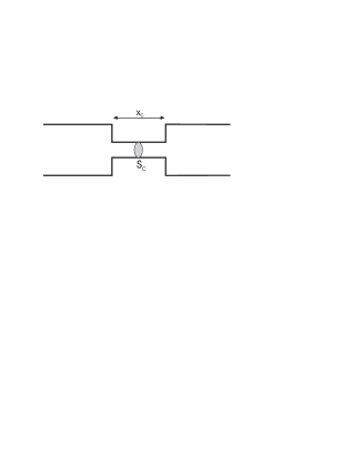
Figure 2: Superconducting nanowire containing a thinner part (constriction) of length $x_{c}$ and cross section $s_{c}$.

Although for homogeneous (at scales $\gtrsim l$) and uniform wires QPT is of the BKT universality class and the temperature dependence of the resistance in the ordered (superconducting) phase is given by eq. (155), there exist other situations in which the dependence (159) may apply at not very low $T$. Consider, e.g., a long superconducting wire with cross-section $s$ and length $X$ which is uniform everywhere except a small part (constriction) of length $x_{c}\ll X$ and cross-section $s_{c}<s$, as shown in Fig. 2. QPS would then occur easier inside the constriction than in the rest of the wire. Assuming for simplicity that $x_{c}$ is of order of (or just slightly larger than) $\xi$, for the corresponding QPS fugacity inside the constriction area we obtain

$$y_{c}\sim S_{\mathrm{core}}(s_{c}/s)\exp(-S_{\mathrm{core}}(s_{c}/s)),$$ (160)

where $S_{\mathrm{core}}$ is the QPS core action (123) for the wire. As before, we can express the partition function $Z$ in terms of series in powers of the QPS fugacity (cf., eq. (129)) which is now equal to $y_{c}$ inside the constriction and to $y$ otherwise. In other words, we should now deal with two different types of logarithmically interacting QPS. Quantum phase slips in the wire are treated exactly as before, and we again arrive at the BKT-like QPT at $\mu=\mu^{\ast}\approx 2$. QPS inside the constriction interact logarithmically only in time, thus giving rise to the Schmid-like QPT at $\mu=1$. In this case the quasi-1D superconducting wire with Mooij-Schön plasmons as elementary excitations plays the role of an effective dissipative environment for the constriction. Such QPT was discussed by Hekking and Glazman HG in the case of a narrow superconducting ring interrupted by the Josephson junction. In the situation considered here this QPT appears to be of little importance since $\mu^{\ast}>1$, i.e. at $T\rightarrow 0$ BKT-like QPT occurs when quantum phase slips inside the constriction are still bound in pairs.

On the other hand, at not very low temperatures and provided $y_{c}\gg y$ quantum phase slips inside the constriction may give an additional contribution to the wire resistance with the temperature dependence (159). In order to demonstrate that we modify eq. (152) by taking into account the difference between QPS fugacities in the wire and in the constriction. This is trivially handled by splitting the space integrals into those over the wire and constriction areas. As a result, the linear resistance of the system becomes

$$R(T)=R_{w}(T)+R_{c}(T),$$

where $R_{w}(T)$ is determined by QPS inside the wire (155), i.e. $R_{w}(T)\propto y^{2}T^{2\mu-3}$, while the additional contribution $R_{c}(T)$ comes from QPS inside the constriction. This contribution has the form $R_{c}(T)\propto y^{2}_{c}T^{2\mu-2}$. Hence, at sufficiently high temperatures the constriction contribution $R_{c}(T)$ can dominate over $R_{w}(T)$, in which case the dependence (159) applies. However, at lower temperatures $R_{c}(T)$ becomes irrelevant and $R(T)$ again is determined by eq. (155). Obviously, the same arguments hold in the case of several constrictions or, more generally, for some wires with strongly fluctuating cross-section. A similar scenario was recently discussed in Ref. Pai where Gaussian fluctuations of the wire thickness were considered.

Finally, let us briefly address the non-superconducting phase $\mu<\mu*$. In our opinion, frequently used oversimplified approaches, like TDGL or effective Luttinger liquid models, are by far insufficient in order to judge whether this disordered phase is actually metallic or insulating, i.e. whether we are dealing with SMT or SIT at $T=0$ and $\mu=\mu^{*}$. Also RG equations (148) cannot unambiguously resolve this issue. To illustrate this point let us compare the behavior of Josephson chains and homogeneous wires. The QPS fugacities $y$ of both systems obey RG equations (148) and, hence, for $\mu<\mu^{*}$ these fugacities grow upon renormalization in both cases. In the case of Josephson chains it only implies strong fluctuations of the phases across barriers with no suppression of superconductivity inside metallic grains. In this case inter-grain tunneling of Cooper pairs is prohibited by electron-electron interactions and the system is in the insulating (Coulomb blockade) phase.

On the contrary, large renormalized QPS fugacity $y$ in the case of homogeneous wires implies that the QPS gas becomes dense, the QPS cores overlap and, hence, for $\mu<\mu^{*}$ and $T\to 0$ superconductivity gets eventually destroyed everywhere in the wire. In other words, in this regime quantum fluctuations drive homogeneous ultra-thin superconducting wires normal. This important difference between homogeneous and granular wires was emphasized in Ref. ZGOZ . What remains is to figure out whether such normal diffusive wires stay metallic or turn insulating at low enough $T$.

Few years after the work ZGOZ it was realized that, similarly to highly conducting tunnel barriers PZ91 ; GZ94 ; GZ94-1 disordered metallic wires with large conductances also demonstrate the feature of weak Coulomb blockade Naz ; GZ00 ; GZ04 ; GZ04-1 ; BN caused by non-trivial interplay between scattering and electron-electron interactions. The presence of an (exponentially small) Coulomb gap implies that disordered wires most likely turn insulating at $T=0$. However, in generic metallic wires with many conducting channels such a state can only be observed at exponentially low $T$, while for any experimentally attainable temperature one expects a metallic behavior with a weak trend for the wire resistance to grow with decreasing $T$ due to Coulomb blockade corrections GZ00 . Interestingly, such a trend was indeed observed in recent experiments Bezryadin MoGe TAPS EPL-2006 ; Bezryadin condmat07 ; Bezryadin MoGe review JPCM 2008 and the measured dependence $R(T)$ was found to closely follow theoretical predictions GZ00 . Further theoretical analysis of the role of electron-electron interactions in quasi-1D structures Bezryadin MoGe TAPS EPL-2006 ; Bezryadin condmat07 ; Bezryadin MoGe review JPCM 2008 would be highly desirable GZ06 .

VI Experiments on superconducting nanowires

VI.1 General considerations

It follows from our theoretical analysis that both TAPS and – in particular– QPS can be observed in sufficiently thin superconducting wires, i.e. experiments aimed to observe QPS-related phenomena should be performed on samples with smallest possible cross section values $s$. On top of that, it is highly desirable to deal with structurally (and chemically) homogeneous samples in order to eliminate spatial variations of $T_{C}$ along the wire and rule out the effect of (possibly existing) constrictions and tunnel barriers. It has been shown that structural imperfections of real quasi-1D structures (non-uniform cross section, existence of probes and finite length effects) might effectively mask the phenomena related to thermal or quantum fluctuations Zgirski inhomogeneity PRB .

In addition to the above requirements, in order to provide optimal conditions for observation of fluctuation effects it is crucial to properly choose the sample material. This is obvious from the fact that, for instance, the QPS core action (123) at low enough $T$ can be represented in the form

$$S_{\mathrm{core}}\sim T_{C}^{1/2}s/\rho_{N},$$

where $\rho_{N}\equiv 1/\sigma$ is the wire resistivity in the normal state. Hence, it is desirable to select superconducting materials with smaller values of $T_{C}$ (or $\Delta_{0}(0)$) and perform experiments on sufficiently dirty nanowires with higher values of $\rho_{N}$. The latter requirement is in line with the well known general observation that fluctuation effects are more pronounced in dirtier systems. This requirement also implies that the electron elastic mean free path should obey the “dirty limit” condition $l<\xi\sim\sqrt{l\xi_{0}}$ where $\xi_{0}\sim\hbar v_{F}/\Delta_{0}$ is the BCS “clean” coherence length. The parameters for various conventional superconductors are listed in Table I. Judging from these numbers the most suitable materials for experimental investigations of QPS effects are those with higher resistivity values, i.e. $MoGe$ and $\alpha$:InO. On the other hand, a certain disadvantage of these materials is that theu can be strongly inhomogeneous. In this respect, Zr or Ti can be advantageous for experimental studies of quantum fluctuations.

Though measuring the temperature dependence of the system resistance $R(T)$ in the vicinity of the transition point might seem a routine experimental task, in the case of nanostructures more care is required. Typically, $R(T)$ dependencies are measured in the current-biased regime. A standard requirement is to keep the bias current $I$ much smaller than the critical (depairing) current $I_{C}$ in order to avoid hysteresis effects due to overheating. Additionally, in order to stay within the linear response regime, the measuring current $I$ should remain smaller than the charactristic scale $I_{0}=k_{B}T_{C}/\Phi_{0}$ la ; mh equal to few tens of nA for the majority of materials (see Table I). The characteristic normal state resistance of a typical metallic nanowire with diameter $\sqrt{s}\simeq$ 10 nm and length $X$ $\simeq$ 1 $\mu$m is of order few k$\Omega$. Hence, in the normal state the expected voltage is at least few $\mu$V, which is certainly not a problem to measure. However, with decreasing temperature only slightly below $T_{C}$ the resistance $R(T)$ drops exponentially and the measured signal quickly reduces to the nV range. Employing room-temperature electronics, it is preferable to use ac lock-in technique in order to increase the signal-to-noise ratio. This can be associated with some hidden problems. One of them is that even a tiny fraction of dc component (e.g. from the ground loop) adds a parasitic signal $\sim dV/dI(T)$ to the ”valuable” one $R(T)\equiv V(T)/I$. For this reason it is advisable to decouple the ac current source from the sample using a low-noise transformer.

Material	$T_{c}$	$\lambda_{0}$	$\xi_{0}$	$B_{c}(0)$	$\Delta(0)$	$v_{F}$	$\rho_{N}$
	$K$	$nm$	$\mu m$	$mT$	$\mathit{meV}$	$10^{6}$ $m/s$	$\mu\Omega\times cm$
W	0.015	-	165*	0.1	0.002*	1.8*	5.7
Ir	0.11	-	22.5*	1.6	0.017*	1.8*	5.1
Hf	0.13	-	19.0*	1.3	0.020*	1.8*	35
Ti	0.40	-	6.2*	5.5	0.061*	1.8*	42.0
Zr	0.61	-	4.0*	4.7	0.093*	1.8*	44.0
Zn	0.86	28	1.8	5.5	0.120	1.82	5.9
Al	1.19	16	1.6	10	0.175	2.02	2.7
$\alpha$:InO	2.8	-	0.330	-	0.430*	-	3000
In	3.41	65	0.360	28	0.520	1.74	8.4
Sn	3.73	50	0.230	30.5	0.557	1.88	11.0
MoGe (film)	5.5	720	0.005	66	1.1	-	200
Pb	7.2	40	0.090	80.3	1.365	1.82	20.7
Nb	9.25	85	0.030	206	1.520	1.37	12.5

Table-I. Material parameters of several superconductors. The data are taken from Refs. Tinkham superconductivity book ; Superconductor Material ; Kittel solid state ; Ashcroft - Mermin ; for $MoGe$ from Refs. Lau MoGe PRL ; Bezryadin private ; Lau privat and for $\alpha$:InO from Refs. Johansson InO nanowire ; Johansson privat . The numbers marked with * are estimated values.

Another problem might originate from the presence of rf filters which are mandatory to protect nano-sized samples from noisy electromagnetic environments. Very often such filters are just RLC circuits shunting the rf component to the ground through a capacitor as high as few $\mu F$. Such configuration might provide good results with high-Ohmic systems (e.g. tunnel structures). In a superconducting nanowire measured in 4-probe configuration each electrode contacting the ”body” of the sample is typically made of the same material. Hence, the resistance of these probes also varies from few k$\Omega$ down to zero over the same temperature range within the transition. Depending on particular configuration, at a certain $T$ the ac sample impedance might become comparable to that of the current leads through the ground, causing the current re-arrangement throughout the sample. Even at rather low measuring frequencies $\sim$ 10 Hz the parasitic effect might manifest itself as a non-monotonous $R(T)$ dependence with unusual ”bumps” or ”foot” at the bottom of the transition. Additional complication might arize from the non-negligible dependence of the gain of the nanovolt pre-amplifier on the total impedance of the load.

Concluding this part, an experimentalist should be extremely cautious in designing the measuring set-up for unambiguous interpretation of the data on superconducting nanowires.

Structural and geometrical homogeneity of quasi-1D samples is the central question in interpretation of experimental data related to contribution of superconducting fluctuations. Theoretically one usually assumes that (i) the critical temperature $T_{C}$ of quasi-1D wires under consideration remains spatially constant, i.e. it does not vary along the wire, (ii) the cross section $s$ does not vary along the wire either and (iii) the measuring probes are non-invasive. Unfortunately, in realistic nanowires none of these conditions is usually well satisfied. To which extent can these imperfections be neglected while interpreting the experimental data using models developed under the assumptions (i)-(iii)?

If structural imperfections (e.g. non-uniform chemical composition) can alter the critical temperature, then the shape of the experimentally observed $R(T)$ dependence is determined by the sequence of transitions of various parts of the wire with different local critical temperature $T_{C}(x)$ . If the degree of such inhomogeneity is not too strong, a step-like $R(T)$ transition may not be observed as the variations of the critical temperature are averaged on the scale of the coherence length $\xi$ resulting in a relatively wide ”smooth-looking” $R(T)$ dependence.

One might naively expect that working with superconducting samples fabricated of initially pure material can help to eliminate the problem. Unfortunately this is not the case. First, properties of low-dimensional superconductors are known depend on the fabrication process details, such as thin film deposition rate, residual pressure in the vacuum chamber, material of the substrate etc. Second, even if to make an effort to keep the fabrication parameters constant, it is hard to get rid of size-dependent effects.

It is a well-known experimental fact that the critical temperature $T_{C}$ of thin superconducting films frequently differs from one for bulk samples. The same tendency is observed in metallic nanostructures. In indium, aluminum and zink $T_{C}$ increases with decreasing characteristic dimension Giordano QPS PRL 1988 ; Zgirski NanoLett 2005 ; Zgirski QPS PRB 2008 ; Altomare Al nanowire PRL 2006 ; Tian Zn nanowire PRL 2005 . On the contrary, in lead, niobium and MoGe an opposite tendency is observed BT ; Bezryadin MoGe TAPS EPL-2006 ; Dynes QPS PRL 1993 ; Bezryadin Nb nanowires ; Bezryadin MoGe and Nb wires . No noticeable variations of $T_{C}$ were detected in tin nanowires Tian Sn nanowire APL 2003 ; Tian Sn nanowire PRB 2005 ; Piraux Sn nanowire APl 2004 ; Piraux Sn nanowire NanoSci NanoTech 2005 . The origin of this phenomenon is not clear. There exist models predicting both suppression Fin and enhancement Shanenko Tc(size) PRB 2006 of the mean field critical temperature for low dimensional superconductors. One can take the empirical fact of variation of $T_{C}$ with effective diameter of a superconducting nanowire as granted. Using $Al$ lift-off fabricated nanowires as a representative example (Figs. 3 and 4) it has been shown that size-dependent effects are extremely important for interpretation of fluctuation phenomena in quasi-1D systems Zgirski inhomogeneity PRB . The conclusion of a quantitative analysis Zgirski inhomogeneity PRB is rather disappointing: even chemically pure nanostructures cannot be considered as sufficiently homogeneous as soon as the size dependence of the critical temperature $T_{C}$ comes into play. One should study atomically homogeneous systems as single crystalline whiskers Webb R(T) in Sn whiskers ; Tinkham R(T) in Sn whiskers . Unfortunately, modern nanotechnology does not enable growth of high-quality quasi-1D single crystalls of arbitrary diameter made of all materials of interest. The lithographic processes results in much lower quality samples. The only exception are materials, such as $Al$, $Zn$ and $In$, where the critical temperature decreases with reduction of the effective dimension (e.g., nanowire diameter). Under certain conditions, experiments on lift-off fabricated nanowires made of these materials can be interpreted using fluctuation models developed for perfect 1D channels. Provided broadening of the $R(T)$ dependencies is detected below the bulk critical temperature $T_{C}^{bulk}$, the size effects cannot account for the phenomenon, and presumably ”real” physics is observed.

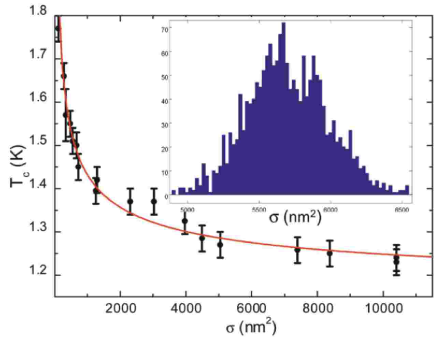
Figure 3: Empirical dependence of the critical temperature $T_{C}$ on cross section $\sigma\equiv s$ for aluminum nanowires. Line is a guide for the eye. Inset: SPM measured distribution of cross sections for a typical lift-off fabricated nanowire: length $X$ =10 $\mu$m and effective diameter $\sqrt{s}\approx$ 75 nm Zgirski inhomogeneity PRB .

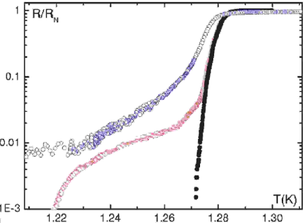
Figure 4: Bullets ($\bullet$) correspond to simulated $R(T)$ transition without taking into consideration the nodes. Diamonds ($\diamond$) represent the results of similar calculations with contribution of the node regions. Open circles ($\circ$) denote the experimentally measured $R(T)$ dependence. Simulations and experimental data are for the same wire as in the inset from the previous figure Zgirski inhomogeneity PRB .

VI.2 Experiments on TAPS

As we have already discussed in Chapter 4 the TAPS mechanism provides non-zero voltage drop across the superconducting wire at temperatures below $T_{C}$. For reference purposes let us rewrite again the expression for the $I-V$ curve derived in the presence of TAPS at sufficiently low bias currents $I$. Combining eqs. (104) and (108) and restoring some fundamental constants (set equal to unity in our theory analysis) we obtain

$$V=\frac{4\sqrt{3\pi}}{e}k_{B}T\frac{X}{\xi(T)}\sqrt{\frac{\delta F}{k_{B}T}}\exp\left[-\frac{\delta F}{k_{B}T}\right]\sinh\left[\frac{\pi\hbar I}{2ek_{B}T}\right],$$

where $\xi(T)$ is the temperature-dependent coherence length of a dirty wire, $k_{B}$ is the Boltzmann constant,

$$\delta F=\frac{16\pi^{2}k_{B}^{3/2}}{21\zeta(3)}sN_{0}\sqrt{\pi\hbar D}(T_{C}-T)^{3/2}$$

is the the potential barrier for TAPS and $\zeta(3)\simeq 1.202$.

Very quickly after development of the LAMH theory la ; mh two experimental groups reported experiments aimed at verification of the TAPS model. At 70-s microfabrication technique was not much developed. In these early studies of 1D superconductivity Webb R(T) in Sn whiskers ; Tinkham R(T) in Sn whiskers metallic whiskers (Fig. 5) with characteristic diameter $\sim$ 1 $\mu$m and lengths up to 1 mm were utilized. Growth and basic properties of these highly anisotropic objects have been widely described in the literature Givargizov whisker growth . In the particular case of tin whiskers ”squeeze” method was typically applied for their growing Fisher whisker growth . Then the crystals were literally hand picked from the ingots and positioned on substrates. The electrodes were made either by conducting paste or epoxy Lutes Sn filaments , soldered by Wood’s metal Meyer IV ; Webb R(T) in Sn whiskers or Sn-Pb alloy Tinkham R(T) in Sn whiskers , or squeezed by a soft metal (e.g. indium) Gaidukov whiskers . An obvious disadvantage of the procedure is inevitable damage of the crystal within the locus of the electric probes. An attempt to overcome these difficulties was made by combining planarization technique with electron beam lithography Arutyunov SOG whiskers ; Arutyunov patents in nanotechnology (Figs. 5 and 6). The technique appears promising, but extremely time consuming and resulting in a rather low yield of ”working” samples.

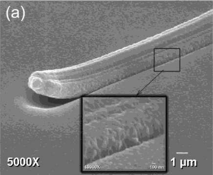
Figure 5: SEM image of a typical tin whisker on the surface of spin-on-glass Arutyunov SOG whiskers . Inset shows the magnified view of the crystal surface Arutyunov patents in nanotechnology .

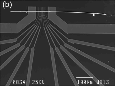
Figure 6: SEM image of a whisker-based microstructure on Si/SiO substrate covered with Spin-On-Glass. Slightly bent bright horizontal line is the tin whisker. Electrodes are made on top of the crystal by e-beam lithography followed by evaporation of copper contacts Arutyunov SOG whiskers .

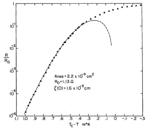
Figure 7: $R(T)$ dependence for a tin whisker Webb R(T) in Sn whiskers . Solid symbols are the experimental data, dashed line represents the fit to the TAPS model la ; mh .

An example of experimental $R(T)$ dependence measured on tin whisker is shown in Fig. 7. One observes a very good quantitative agreement between the experiment Webb R(T) in Sn whiskers ; Tinkham R(T) in Sn whiskers and the TAPS model la ; mh . The superconducting transition $R(T)$ is very steep: resistance of the sample drops five orders of magnitude within the temperature range $\delta T$ $\sim$ 1 mK below $T_{C}$. This is a consequence of rather large effective diameter values $\sqrt{s}\simeq 0.5$ $\mu$m and extremely high homogeneity of single crystals. In the case of thinner single-crystalline structures the width of the $R(T)$-curve would be larger, cf. eq. (109). Unfortunately, the dimensions of whiskers made of superconducting materials do not vary much. Manual manipulation of sub-1 $\mu m$ is extremely time consuming and results in a low yield of suitable samples, while the dimensions of whiskers are still too large to use scanning probe (SPM) technique well developed for manipulation of nano-sized objects, such as carbon nanotubes.

An alternative to whiskers is superconducting microcylinders encapsulated in a dielectric substrate (e.g. glass) fabricated using Taylor-Ulitovski method Taylor micricylinder method ; Taylor microcylinder patent ; Ulitovski microcylinder method ; Ulitovski microcylinder patent1 ; Ulitovski microcylinder patent2 . The quality of these wires is not as high as that of atomically-pure whiskers. However, an important advantage of this approach is the possibility to fabricate very long samples. Fabrication of a wire with metal core of about few $\mu$m and length up to a km (!) is a routine work, while fine adjustment of parameters enables fabrication of sub-100 nm filaments with length up to few cm Nikolaeva sub 1 mkm Bi wires ; Nikolaeva Bi-Te nanofilaments ; Nikolaeva confinement in Bi nanowires . A remarkable feature of wires obtained by this method is that typically they are single crystals. A number of superconducting microcylinders (Sn and In) fabricated using Taylor-Ulitovski method were studied Arutyunov Sn and In filaments JAP ; Arutyunov Sn and In filaments Physica C . Bigger length values of the filaments ($X\sim$ 1 cm ) as compared to those for previously studied whiskers ($X\sim$ 0.5 mm ) enabled observation of interesting features related to interaction of current-induced phase slips. The cross section values for microcylinders did not differ much from those for whiskers, while the homogeneity was clearly worse: No qualitatively new phenomena related to fluctuation-governed 1D superconductivity has been observed.

There were several reports on experimental studies of 1D superconductivity in lift-off-fabricated superconducting nanostructures (wires and loops) with the line-width much smaller than of whiskers or microcylinders Santhanam nMR anomaly ; Santhanam R(T) anomaly ; Moschalkov Little-Parks anomaly ; Moshchalkov R(T) anomaly ; Arutyunov non-locality . The advantage of the method is the ability to fabricate samples with a complicated shape in a reproducible way. Typically, the metal is deposited through PMMA mask using thermal or e-beam evaporation, or sputtering. The quality of the structures is far from perfect: the majority of superconducting thin-film structures fabricated at room temperatures are polycrystalline with the grain size of about few tens of nm. Deposition of metal (in particular low melting ones, such as tin or indium) on a cryogenically cooled substrate might reduce the grain size. In contrast to whiskers or microcylinders, the lift-off-fabricated superconducting nanostructures studied so far were all in the dirty limit $l\ll\xi$. Attempts to quantitatively describe the shape of superconducting transition of these quasi-1D systems using the TAPS model failed: Experimental curves for $R(T)$ were always significantly broader than theoretical predictions. Nevertheless, it was believed that with a certain adjustment of fit parameters (e.g., reduction of the effective size of the phase slip center Moshchalkov R(T) anomaly ) a reasonable agreement between the experiments and the TAPS model predictions could be achieved. Later it was shown that inevitable inhomogeneity of lift-off-fabricated nanostructures, the presence of node regions and finite size effects can dramatically broaden the experimentally observed dependencies $R(T)$ making any comparison with the TAPS theory inconclusive or even impossible (Fig. 4) Zgirski inhomogeneity PRB .

Very thin superconducting nanowires have been studied using the template decoration technique: Deposition of a metal film on top of a suspended insulating molecule used as a template Bezryadin molecular decoration 1 ; Bezryadin molecular decoration 2 ; Bezryadin molecular decoration 3 ; Johansson InO nanowire (Fig. 8). Only pseudo-four probe configuration is available with the deposited metal film from both sides of the trench serving as electrodes. The approach enabled fabrication of superconducting nanowires (MoGe, Nb and $\alpha$:InO) with effective diameters down to $\sim$3 nm and lengths up to $\sim$1 $\mu$m. TEM study revealed amorphous structure for MoGe and $\alpha$:InO.

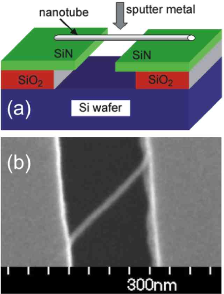
Figure 8: Molecular template decoration method. (a) Schematics of the fabrication technique. (b) SEM image of a carbon-nanotube-based structure Bezryadin molecular decoration 1 , Bezryadin molecular decoration 3 .

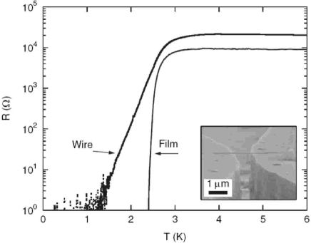
Figure 9: $R(T)$ obtained from $\alpha$:InO nanowire with width 100 nm together with the data from a similarly prepared 500 $\mu$m wide film. Inset: A scanning electron micrograph (SEM) of a typical device Johansson InO nanowire .

The $R(T)$ dependencies in $\alpha$:InO appeared to be significantly wider than it is predicted by the TAPS model, though no claims about the impact of the QPS mechanism were made Johansson InO nanowire . Possibly, broadening of experimental curves $R(T)$ in $\alpha$:InO can be associated with inevitable inhomogeneity of the samples introduced during their fabrication. It is well known that physical properties of $\alpha$:InO low dimensional systems strongly vary by annealing InO film Shahar PRB 1992 .

Interpretation of some experiments on MoGe nanowires remains under debates. In earlier reports BT ; Lau MoGe PRL very broad $R(T)$ dependencies were observed and associated with quantum phase slips. However, in later works Bezryadin MoGe and Nb wires ; Bezryadin MoGe TAPS EPL-2006 ; Bezryadin MoGe review JPCM 2008 ; Bezryadin condmat07 broadening of a superconducting transition in similar MoGe structures was interpreted within the TAPS model with no QPS contribution (Fig. 10). On the other hand, later it was argued Meidan ; Meidan2 that fits were actually produced outside the applicability range of the LAMH theory (105). Moreover, for the experimental parameters Bezryadin MoGe and Nb wires ; Bezryadin MoGe TAPS EPL-2006 ; Bezryadin MoGe review JPCM 2008 ; Bezryadin condmat07 the strong inequalities (105) are not satisfied, i.e. this theory has almost no applicability range at all, see also Fig. 11. Thus, employing the LAMH model in order to fit the resistance curves $R(T)$ for these samples is problematic. In addition, even if one performs such fits one is bound to use fit values for the electron mean free path much larger than the wire diameter Bezryadin MoGe TAPS EPL-2006 which is rather unrealistic for such structures (Fig. 10). At this point let us recall that estimates for the coherence length $\xi(0)\sim(\xi_{0}l)^{1/2}$ both in MoGe thin films Graybeal QPS in MoGe PRL 1987 ; Graybeal 2D MoGe films PRB 1984 and wires BT typically yield values $\sim 5$ to 7 nm which translates into mean free path values $l$ of only few nm, i.e. much shorter than used in the fits Bezryadin MoGe TAPS EPL-2006 . We will return to possible interpretation of these experiments below in connection with QPS effects.

Transmission electron microscopy (TEM) study of Nb nanowires, fabricated using template decoration method, revealed polycrystalline structure with an average grain size about few nm. In order to fit the data obtained in these Nb structures it has been proposed Lau MoGe PRL to represent the measured wire conductance $1/R(T)$ as a sum of contributions from normal electrons above the gap and from TAPS, $1/R(T)=1/R_{N}+1/R_{TAPS}$. The experimental curves $R(T)$ could be reasonably well fitted Bezryadin Nb nanowires ; Bezryadin MoGe and Nb wires to this phenomenological model (Fig. 12). Still, the ability to detect TAPS contribution in Nb is rather unexpected since the energy gap $\Delta_{0}$ is very large in this material (see Table I). It is also quite surprising that the inhomogeneities in granular Nb nanowires do not seem to broaden the $R(T)$ curves, which can be fitted by the TAPS model developed for homogeneous quasi-1D systems.

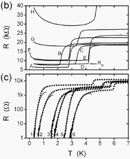
Figure 10: Resistance versus temperature plots for ”short” MoGe nanowires: insulating (top) and superconducting (bottom) Bezryadin MoGe TAPS EPL-2006 . Solid lines are fits to the TAPS model. The best fit values of the coherence lengths $\xi(0)$ are 70.0, 19.0, 11.5, 9.4, 5.6, and 6.7 nm, and lengths $L$ are 177, 43, 63, 93, 187, 99 nm for samples 1–6, respectively. Double-step shape of $R(T)$ transitions in the top and bottom plots comes from the superconducting transition of the contact regions contributing to the 2-probe measurement configuration.

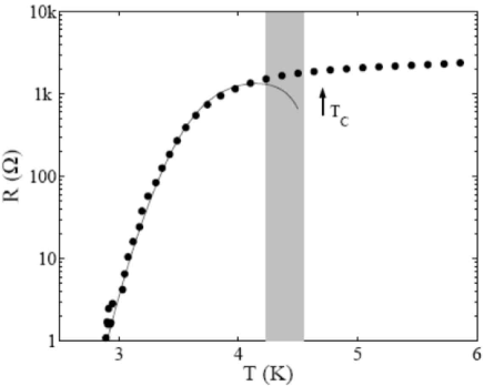
Figure 11: Fits of the data points for the sample No. 6 of Ref. Bezryadin MoGe TAPS EPL-2006 to the LAMH theory. The fit parameters are the coherence length, $\xi$ = 6.7 nm, and the critical temperature, $T_{C}$ = 4.7 K, marked by an arrow. The LAMH theory can only be applied within the strip 4.23 K $<T<4.55$ K Meidan ; Meidan2 (shown in grey) which is clearly outside the region where $R$ strongly depends on temperature.

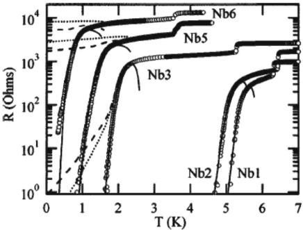
Figure 12: Temperature dependence of the resistance of superconducting Nb nanowires obtained by template decoration method using carbon nanotube as a substrate. The following fit parameters for the samples Nb1, Nb2, Nb3, Nb5, and Nb6 are used: Transition temperatures (K) are $T_{C}^{wire}$ = 5.8, 5.6, 2.7, 2.5, and 1.9 K; lengths (nm) are $X$ = 137, 120, 172, 177 and 113; normal state resistance ($\Omega$) are $R_{N}$ = 470, 650, 1600, 4250 and 9500; coherence lengths (nm) are $\xi(0)$= 8.5, 8.1, 18, 16, and 16.5, respectively. Solid lines show fits to the phenomenological TAPS model Lau MoGe PRL . The dashed and dotted lines are some theoretical curves that include QPS contributions.

VI.3 Experimental observations of QPS effects in superconducting nanowires

Let us now turn to the experiments detecting QPS effects in superconducting nanowires. Mooij and coworkers Mooji discussed the possibility to observe quantum phase slips experimentally and attempted to do so as early as in 1987. According to our theory, the crossover between TAPS and QPS regimes can be expected at temperatures $T\sim\Delta_{0}(T)$. For superconductors with typical material parameters and $T_{C}\gtrsim$ 1K (see Table I) this condition implies that QPS effects may become important already at $T_{C}-T\gtrsim$ 100 mK. As we already discussed, in order to be able to observe QPS it is necessary to fabricate nanowires with effective diameters in the 10 nm range, $\sqrt{s}\sim$ 10 nm. The wires should be sufficiently uniform and homogeneous in order not to override fluctuation effects by trivial broadening of $R(T)$ dependencies due to wire imperfections and inhomogeneities Zgirski inhomogeneity PRB . Thus, proper fabrication technology is vitally important for experimental studies of QPS in quasi-1D superconductors.

Perhaps the first experimental indication of the effect of quantum fluctuations was obtained in amorphous MoGe nanowires with effective diameter down to $\sqrt{s}\simeq$ 30 nm Graybeal QPS in MoGe PRL 1987 . The samples in 4-probe configuration with length $X$ up to 20 $\mu$m were fabricated using e-beam lithography. Though the paper Graybeal QPS in MoGe PRL 1987 was mainly focused on the effect of disorder in low-dimensional superconductors, it was clearly stated that for the narrowest samples significantly broader curves $R(T)$ were observed than it is predicted by the TAPS model (see Fig. 13). The effect of quantum fluctuations was pointed out as a possible reason for this disagreement.

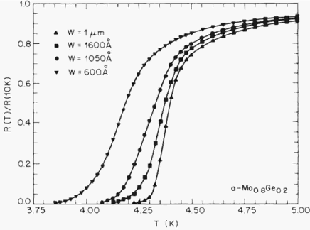
Figure 13: Resistive transitions for a set of MoGe wires with different width $w$ upon a single film of thickness $t=5$ nm Graybeal QPS in MoGe PRL 1987 .

Detailed experimental studies of transport properties of superconducting nanowires have been carried out by Giordano and co-workers Giordano QPS PRL 1988 ; Giordano QPS PRL 1989 ; Giordano QPS PRB 1991 ; Giordano Physica B 1994 ; Giordano QPS PRB 1990 . In these experiments In and In-Pb wires with triangular cross-section were fabricated using step-edge lithographic technique Giordano step technique APL 1980 ; Girdano step technique PRL 1979 . This method utilizes the shadow effect produced by extremely shallow steps in substrates and the corresponding tilted ion beam milling of the deposited material (Fig. 14). Polycrystalline wires were fabricated with effective diameters $\sqrt{s}$ in the range 40 - 100 nm with the grain size from 10 to 20 nm. The uniformity of the samples was controlled with SEM and with the accuracy of $\sim 10$ nm.

Figure 14: Step decoration technique Girdano step technique PRL 1979 .

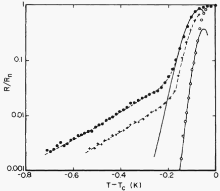
Figure 15: Resistance (normalized by its normal state value) as a function of temperature for three In wires; the sample diameters were 41 nm ($\bullet$), 50.5 nm ($+$) and 72 nm ($\circ$). The solid curves are fits to the TAPS model, while the dashed curves indicate fits to the phenomenological model Giordano QPS PRL 1988 . The sample lengths are 80, 150 and 150 $\mu$m, and the normal state resistance values are 5.7, 7.1 and 1.2 k$\Omega$, respectively Giordano QPS PRL 1988 .

For wider structures a reasonable agreement with the TAPS model was observed. On the other hand, for thinner wires with $\sqrt{s}\lesssim$ 50 nm clear deviations from TAPS predictions were demonstrated (see Fig. 15). The discrepancy was interpreted as a manifestation of quantum phase slippage. In order to explain their observations Giordano and co-workers proposed phenomenological description based on the Caldeira-Leggett model for macroscopic quantum tunneling with dissipation cl . Though qualitative agreement with this simple phenomenological model has been obtained (Fig. 15), quantitative interpretation of the data Giordano QPS PRL 1988 is problematic due to poor uniformity of the samples: $\pm$ 10 nm for wires with $\sqrt{s}\lesssim$ 50 nm Giordano QPS PRL 1988 .

Recently, Pai et al. Pai performed a fit of the same experimental data Giordano QPS PRL 1988 to the power-law dependence $R(T)\propto T^{2\mu-2}$ derived from the result (155) assuming Gaussian fluctuations of the wire thickness. Unfortunately the temperature dependence of the QPS fugacity (146) was not taken into account in Ref. Pai . This temperature dependence (predominantly determined by that of the gap, $S_{\mathrm{core}}\propto\Delta_{0}^{1/2}(T)$) should, however, still be significant at temperatures not very far from $T_{C}$ and will alter the fits.

It appears that strong granularity of the wires was most likely a very important factor in the experiments by Giordano and co-workers. For instance, estimating $S_{\mathrm{core}}$ for the thinnest wires Giordano QPS PRB 1991 with diameters 16 and 25 nm, for the experimental parameters we obtain respectively $S_{\mathrm{core}}\sim 280A$ and $\sim 700A$. For uniform wires such huge values of the QPS action would totally prohibit any signature of quantum phase slips. Since QPS effects were very clearly observed, it appears inevitable that these samples contained constrictions with diameters $\sim 3\div 10$ times smaller than the average thickness values presented in Giordano QPS PRB 1991 .

Another set of experiments was performed by Dynes and co-workers Dynes QPS PRL 1993 ; Dynes QPS and nMR PRL 1997 ; Dynes QPS PRL 1996 . Suspended stencil technique has been developed (Fig. 16 ) enabling fabrication of quench-condensed granular nanowires with cross-section area $s$ down to 15 nm² and length $X$ ranging from 1 to 2 $\mu$m from various materials including several superconductors, such as Pb, Sn, Pb-Bi. The samples edge roughness was claimed to be about 3 nm. A remarkable feature of the method is the ability to vary the wire thickness $t$ and, hence, its cross section $s$ at a constant width $w$ in situ inside the cryostat in-between the sessions of truly 4-probe $R(T)$ measurements.

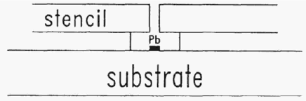
Figure 16: Cross-sectional view of the stencil structure. Metallic films were evaporated through the shadow mask structure fabricated on the substrate Dynes QPS PRL 1993 .

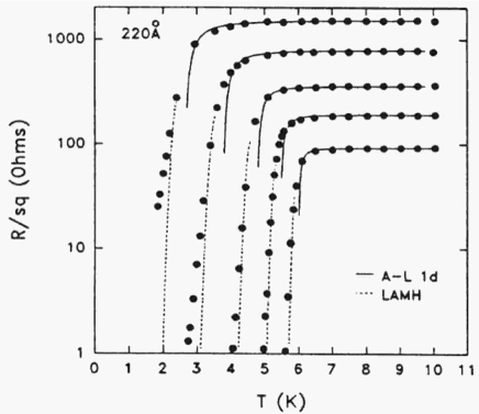
Figure 17: $R(T)$ dependencies for the same Pb nanowire with width $w=$ 22 nm and various thicknesses. Solid lines at the top of the transitions are fits to the Aslamazov - Larkin theory. Dashed lines are fits to the TAPS model, which clearly yields steeper $R(T)$ dependencies compared to the experimental data for the thinnest wires Dynes QPS PRL 1993 .

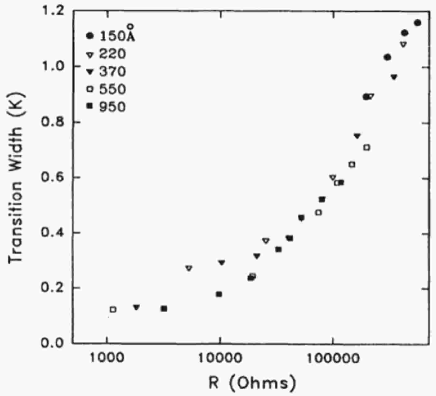
Figure 18: Width of the transition (defined as a temperature interval between 20% and 80% of the normal state resistance Dynes QPS PRL 1993 ) as a function of the normal state resistance $R_{N}$.

The experiments Dynes QPS PRL 1993 clearly indicated systematic deviations of the experimental data points $R(T)$ from the TAPS model predictions (Fig. 17). This discrepancy increases as the wires become narrower. The width of the superconducting transition was found to scale with the normal state resistance $R_{N}$ (Fig. 18). It should be noted that in lead nanowires as narrow as 15 nm and as thin as 10 nm no low temperature resistance tails were observed. Instead, a less dramatic but systematic broadening of the superconducting transition beyond the TAPS limit was noted Dynes QPS PRL 1993 ; Dynes QPS and nMR PRL 1997 . On the other hand, long resistance tails were always present in tin structures fabricated and measured using similar technique Dynes QPS PRL 1996 . Very probably, the discrepancy comes from the difference in the heights of the potential barrier $\delta F$ between these two materials (see Table I): Lead wires should be significantly narrower than tin ones in order to obtain a similar magnitude of fluctuation effects.

In addition, we point out that the experiments Dynes QPS PRL 1993 ; Dynes QPS and nMR PRL 1997 ; Dynes QPS PRL 1996 demonstrated clear superonducting transitions reaching experimental ”zero” in nanowires with normal state resistance $R_{N}\gg$ 10 k$\Omega$. This observation is not in line with the conjecture BT ; Bezryadin MoGe review JPCM 2008 that superconductivity in MoGe nanowires could only be possible for wire resistances below the quantum resistance unit $R_{q}\simeq$ 6.45 k$\Omega$.

A clear manifestation of a crucial role of QPS effects in superconducting nanowires was provided in the experiments by Tinkham and co-workers BT ; Lau MoGe PRL . These authors developed a novel technique which allowed them to fabricate sufficiently uniform superconducting wires considerably thinner than 10 nm with lengths ranging between $\sim 100$ nm and 1 $\mu$m. This was achieved by sputtering a superconducting alloy of amorphous $Mo_{79}Ge_{21}$ over a free-standing carbon nanotube or bundle of tubes laid down over a narrow and deep slit etched in the substrate (Fig. 8). Three out of eight samples studied in the experiments BT demonstrated no sign of superconductivity even well below the bulk critical temperature $T_{C}$. Furthermore, in the low temperature limit the resistance of these samples was found to show a slight upturn with decreasing $T$. In view of that one can conjecture that these samples may actually become insulating at $T\rightarrow 0$. The resistance of other five samples BT decreased with decreasing $T$. Also for these five samples no sharp superconducting phase transition was observed.

All three non-superconducting wires (i1,i2 and i3) BT had the normal state resistance above the quantum unit $R_{q}$, while $R_{N}$ for the remaining five “superconducting” samples was lower than $R_{q}$. This observation allowed the authors BT to suggest that a dramatic difference in the behavior of these two groups of samples (otherwise having similar parameters) can be due to the dissipative quantum phase transition (QPT) ZGOZ2 ; Buchler (see also Chapter 5) analogous to Schmid phase transition sz ; weiss observed earlier in Josephson junctions Mikko . Already at this stage we would like to emphasize that an important pre-requisite for this QPT is the existence of a source for linear Ohmic dissipation at low energies which typically requires the presence of some normal shunt resistance. It appears that no such condition was fulfilled in the experiments BT . Hence, the interpretation of the data BT in terms of a dissipative QPT is problematic.

And indeed, this interpretation was not confirmed in the later experiments of the same group Lau MoGe PRL who observed superconducting behavior in samples with normal resistances as high as 40 k$\Omega$ $\gg R_{q}$. The authors Lau MoGe PRL concluded that ”the relevant parameter controlling the superconducting transition is not the ratio of $R_{q}/R_{N}$, but appears to be resistance per unit length, or equivalently, the cross-sectional area of a wire” (Fig.19).

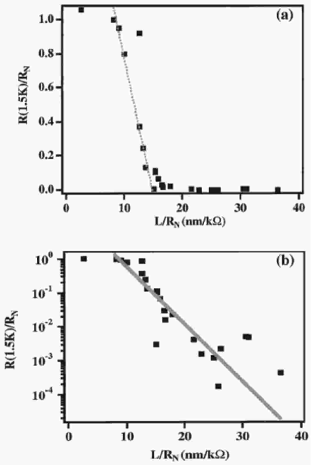
Figure 19: Resistance at 1.5 K normalized to normal state resistance as a function of $L/R_{N}$. (a) Linear plot. The dotted line is a guide to the eye. (b) Semilog plot with an exponential fit. Slope of the fitted line is 0.39 k$\Omega$/ nm Lau MoGe PRL .

This conclusion clearly favors interpretation of the data BT ; Lau MoGe PRL either in terms of a BKT-like QPT ZGOZ ; ZGOZ2 at $\mu\approx 2$ or just as a sharp crossover between the regimes of vanishingly small and sufficiently high QPS rates $\gamma_{QPS}$ which will correspond respectively to superconducting and normal behavior of the nanowires. In both cases the crucial parameter is the wire cross section $s$. Both these QPT and crossover are expected to occur for wire diameters $\sim 10$ nm.

Let us estimate the QPS core action $S_{\mathrm{core}}$ defined by eq. (123) for the eight samples studied in the experiments BT . With the density of states $N_{0}=1.86\times 10^{13}$ s/m³, the superconducting critical temperature $T_{C}\simeq 5.5$ K and the measured resistivity $\rho=1.8$ $\mu\Omega/$m we obtain the coherence length $\xi\simeq 7$ nm in agreement with the estimate BT . Our estimates for the action $S_{\mathrm{core}}$ are summarized in the following Table II:

sample	$R/X$, k$\Omega$/nm	$S_{\mathrm{core}}$
i1	0.122	7.8 $A$
i2	0.110	8.7 $A$
i3	0.079	12.7 $A$
s1	0.038	25.1 $A$
s2	0.028	33.7 $A$
s3	0.039	22.6 $A$
ss1	0.054	15.4 $A$
ss2	0.044	19.6 $A$

We observe that for $A\sim 1$ the QPS rate $\gamma_{QPS}\propto\exp(-S_{\mathrm{core}})$ is expected to be much higher in the normal samples i1, i2 and i3 than in five remaining wires which demonstrated the superconducting behavior in the low temperature limit. This observation is consistent with the interpretation in terms of the crossover between the regimes with low and high QPS rates.

Further support for this interpretation comes from the data Lau MoGe PRL obtained for more than 20 different nanowires. The resistance of these wires measured at $T=1.5$ K is presented in Fig. 19 versus the inverse normal resistance per unit length $X/R_{N}\propto s$. In Fig. 19 (a) one observes a sharp crossover between normal and superconducting behavior at wire diameters $\sqrt{s}\sim 10$ nm. This crossover could be interpreted as an indication to the QPS-binding-unbinding QPT ZGOZ ; ZGOZ2 controlled by the parameter $\mu\propto\sqrt{s}$. Note, however, that all wires studied in Lau MoGe PRL were quite short. Hence, this QPT should inevitably be significantly broadened by finite size effects.

Re-plotting the same data on a semilog scale (Fig. 19 (b)) we indeed observe a rather broad distribution of measured resistances which – despite some scatter – can be fitted to the linear dependence on the wire cross section $s$. This fit is highly suggestive of the crossover scenario although it cannot yet rule out the (broadened by size effects) QPT either.

In order to finally discriminate between these two options it is necessary to analyze the temperature dependence of the resistance $R(T)$. According to our theory, in the linear regime the (caused by QPS) wire resistance is defined by eq. (155). The dependence $R\propto y^{2}$ comes from pairs of QPS events where the fugacity (146) depends on temperature via $S_{\mathrm{core}}\propto\Delta_{0}^{1/2}(T)$. An additional (weak) power-law dependence $\propto T^{2\mu-3}$ enters because of interactions between quantum phase slips in space-time. In order to fit the data Lau MoGe PRL we will ignore this power-law dependence and use the simplified formula

$$R(T)=b_{1}\frac{\Delta_{0}(T)S_{\mathrm{core}}^{2}X}{\xi(T)}\exp(-2S_{\mathrm{core}}),$$ (161)

with $S_{\mathrm{core}}$ defined in (123) and $b_{1}$ being an unimportant constant factor. As this formula can only be applied to samples with vanishing low $T$ resistances $R(T\rightarrow 0)\rightarrow 0$, we select the data Lau MoGe PRL for the samples 3 to 8 seemingly demonstrating such a behavior. The results of the fits to eq. (161) are presented in Fig. 20. We observe a very good agreement between our QPS theory and experiment which was obtained using the same value $A\simeq 0.7$ for all six samples.

We also note that the fits remain essentially unchanged if we take into account an additional power law dependence $\propto T^{2\mu-3}$ (with $\mu$ estimated from the wire parameters). This observation proves that inter-QPS interaction is indeed insignificant for the interpretation of the data Lau MoGe PRL . Thus, similarly to Lau et al. Lau MoGe PRL , we conclude that the temperature dependence of the resistance of their ultra-thin $MoGe$ wires is determined by QPS effects and the observed sharp transition between normal and superconducting behavior is most likely a thickness-governed crossover between the regimes of respectively large and small QPS rates $\gamma_{{}_{QPS}}$.

Figure 20: Superconducting transitions of ”long” MoGe nanowires on top of insulating carbon nanotube used as the substrate BT , Lau MoGe PRL . Double-step shape of the $R(T)$ dependences comes from the superconducting transition of the contact regions contributing to the 2-probe measurement configuration. The samples’ normal state resistances and lengths are 1: 14.8 k$\Omega$, 135 nm; 2: 10.7 k$\Omega$, 135 nm; 3: 47 k$\Omega$, 745 nm; 4: 17.3 k$\Omega$, 310 nm; 5: 32 k$\Omega$, 730 nm; 6: 40 k$\Omega$, 1050 nm; 7: 10 k$\Omega$, 310 nm; 8: 4.5 k$\Omega$, 165 nm. Symbols stand for calculations using eq. 161 with the single numerical coefficient $A$=0.7. The critical temperature $T_{C}$ and the dirty-limit coherence length $\xi(0)$ used as fitting parameters for samples 3-8 are 3: 5.0 K, 8 nm; 4: 6.4 K, 8.5 nm; 5: 4.6 K, 8.9 nm; 6: 4.8 K, 8.9 nm; 7: 5.6 K, 11.9 nm; 8: 4.8 K, 8.5 nm. Data for samples 1 and 2 cannot be fitted by any reasonable set of parameters.

A bulk of recent experimental data Bezryadin MoGe and Nb wires ; Bezryadin MoGe TAPS EPL-2006 ; Bezryadin condmat07 accumulated on MoGe nanowires fabricated using the molecular template method was recently reviewed in detail by Bezryadin Bezryadin MoGe review JPCM 2008 . The main observations can be summarized as follows: ($i$) ”shorter” nanowires ($X\lesssim 200$ nm) demonstrate either ”weakly insulating” behavior with clear features of weak Coulomb blockade Naz ; GZ00 ; GZ04 ; BN , or relatively steep superconducting transition $R(T)$ with virtually no samples showing an intermediate regime, ($ii$) ”longer” samples (200 nm $\lesssim X\lesssim$ 1 $\mu$m) typically showed the behavior which – similarly to the data Lau MoGe PRL – can reasonably well be interpreted in terms of a crossover between the regimes of small and large QPS rates (corresponding to respectively superconducting and normal behavior).

The $R(T)$ curves of longer wires in the regime ($ii$) showed a decrease of the resistance with cooling no matter whether their normal state resistance $R_{N}$ was smaller or bigger than $R_{q}$. The crossover between normal and superconducting behavior of the samples was controlled by the wire cross section $s$ or, equivalently, by the ratio $R_{N}/X$. As in Ref. Lau MoGe PRL , the overall picture is consistent with the QPS scenario GZ01 .

Turning to the regime of shorter wires ($i$), it was argued Bezryadin condmat07 ; Bezryadin MoGe review JPCM 2008 that the transition between superconducting and normal behavior for these samples is most likely controlled by the total normal wire resistance $R_{N}$ rather than by the resistance per unit length $R_{N}/X$, see Fig. 3 of Ref. Bezryadin condmat07 . This observation implies that a significant fraction of short wires with lengths $X\lesssim 200$ nm showed superconducting-like behavior even though the corresponding estimated values of the QPS core action could be as high as $S_{\mathrm{core}}\sim 1$ (in which case for longer wires one expects strong proliferation of QPS leading to total destruction of superconductivity). One should, therefore, explain why these samples stay superconducting instead of being normal or even insulating in the limit of low enough $T$.

An empirical fact that short samples Bezryadin condmat07 ; Bezryadin MoGe review JPCM 2008 stayed normal for $R_{N}\gtrsim R_{q}$ and turned superconducting as soon as $R_{N}\lesssim R_{q}$ allowed the authors to assume the presence of some kind of QPT that could, for instance, be similar to Schmid dissipative phase transition in Josephson junctions s ; Chbm ; sz ; weiss . Thus, in some sense the authors Bezryadin condmat07 revived an earlier idea BT , now in application to short wires only. Supporting this idea Meidan et al. Meidan ; Meidan2 suggested a phenomenological scheme essentially employing the well known RG analysis developed for resistively shunted Josephson junctions s ; sz ; weiss . Unfortunately, as was also noticed in Refs. Meidan ; Meidan2 , the experimental parameters correspond to large fugacity values $y\sim 1$, i.e. the RG approach s was employed in Ref. Meidan ; Meidan2 well beyond its applicability range. Another – even more significant problem – is that in the structures Bezryadin condmat07 ; Bezryadin MoGe review JPCM 2008 no source for linear Ohmic dissipation seems to exist at low energies. Meidan et al. phenomenologically argued that such dissipation could occur due to proliferation of QPS inside the wire (which would make the wire to a large extent normal). However, even intrinsically normal wires in contact with superconducting electrodes develop a proximity-induced gap in its energy spectrum GK ; BBS2 ; Been ; Pilgram ; Zhou ; KKZ of order Thouless energy $\epsilon_{\mathrm{Th}}=D/X^{2}$. Hence, Ohmic dissipation can hardly occur in such SNS structures at energies $\lesssim\epsilon_{\mathrm{Th}}$. Since for short samples Bezryadin condmat07 ; Bezryadin MoGe review JPCM 2008 with $X\sim 40\div 200$ nm the energy $\epsilon_{\mathrm{Th}}$ can easily reach few K, it is hard to expect that a dissipative QPT can occur in such systems.

The same arguments suggest that the proximity effect may actually play an important role in the interpretation of the experimental data Bezryadin condmat07 ; Bezryadin MoGe review JPCM 2008 for short samples. Even if the wire is intrinsically normal, supercurrent can flow through such a weak link due to the proximity effect. Accordingly, superconductivity in the short samples with $R_{N}\lesssim R_{q}$ can simply be associated with the onset of dc Josephson current in an SNS junction. The corresponding scenario is as follows.

In the interesting limit $X\gg\xi$ the Josephson energy $E_{J}(T)$ of an SNS junction FNT ; WZK ; Dubos is exponentially small at high temperatures $T\gg\epsilon_{\mathrm{Th}}$. Hence, at such $T$ we have $E_{J}(T)\ll T$ and the weak Josephson current is fully suppressed by thermal fluctuations. Upon decreasing temperature one eventually reaches the regime $T\lesssim\epsilon_{\mathrm{Th}}$, in which case $E_{J}$ becomes Dubos

$$E_{J}\sim\epsilon_{\mathrm{Th}}R_{q}/R_{N}.$$ (162)

Thus, for $R_{N}\lesssim R_{q}$ at $T\ll\epsilon_{\mathrm{Th}}$ we have $E_{J}\gg T$, i.e. thermal fluctuations are negligible and the SNS junction becomes superconducting. In the vicinity of $T\sim\epsilon_{\mathrm{Th}}$ this argument also allows to predict exponential decrease of the wire resistance $R(T)\propto\exp(\epsilon_{\mathrm{Th}}R_{q}/R_{N}T)$ in a qualitative agreement with exponential dependencies observed in Bezryadin MoGe TAPS EPL-2006 ; Bezryadin MoGe review JPCM 2008 . On the other hand, for $R_{N}\gtrsim R_{q}$ at $T\sim\epsilon_{\mathrm{Th}}$ we still have $E_{J}<T$, i.e. supercurrent is disrupted by thermal fluctuations down to lower $T$ and significantly broader $R(T)$ curves are expected.

At lower $T$ thermal fluctuations become unimportant but, on the other hand, quantum fluctuations take over destroying the Josephson current for $E_{C}\gtrsim E_{J}$, where $E_{C}=e^{2}/2C$ is an effective charging energy of an SNS junction. Thus, in the low temperature limit one would expect to see the crossover at $E_{J}\sim E_{C}$ or, equivalently, at

$$R_{q}/R_{N}\sim E_{C}/\epsilon_{\mathrm{Th}}.$$ (163)

Now, similarly to the case of Josephson junctions sz , one can demonstrate that the capacitance $C$ is given by the expression $C=C_{g}+\delta C$, where $C_{g}$ is the junction geometric capacitance and $\delta C$ is the renormalization term $\delta C\sim\hbar/R_{N}\epsilon_{\mathrm{Th}}$. Since in our case geometric capacitance is most likely very small $C_{g}\ll\delta C$, one has $E_{C}\sim R_{N}\epsilon_{\mathrm{Th}}/R_{q}$. Substituting this estimate into eq. (163), one immediately obtains the crossover condition

$$R_{N}\sim R_{q}$$

in agreement with experimental findings. We believe that these simple arguments are sufficient to understand a superconducting-to-normal crossover observed in short wires Bezryadin MoGe TAPS EPL-2006 ; Bezryadin condmat07 ; Bezryadin MoGe review JPCM 2008 . These arguments also demonstrate that for such samples Josephson physics (both classical and quantum) appears to be more important than that of TAPS and QPS. Hence, although short wires can also demonstrate interesting phenomena, longer wires appear to be more suitable for experimental investigations of QPS effects.

Now let us turn to other experiments where QPS in superconducting nanowires have been observed.

The original method of forcing the molten alloy into a porous media Bogomolov capillary wire Sov Phys Sol St 1971 or capillary Michael In microcylinders JLTP 1974 enables fabrication of metallic wires with diameters $\gtrsim$1 $\mu$m. At these early stages of research no studies of the shape of superconducting transition were performed in such structures. Chemical or electrochemical methods developed later allowed filling of very narrow pores with a wide variety of materials including superconductors: $Pb$ Yi Pb electrodeposited nanowires APL 1999 ; Piraux IV in Pb and Sn nanowire PRL 2003 ; Piraux Pb nanowire PRB 2004 ; Piraux Pb nanowire IV APL 2008 , $Sn$ Piraux Sn nanowire APl 2004 ; Piraux Sn nanowire NanoSci NanoTech 2005 ; Piraux IV in Pb and Sn nanowire PRL 2003 ; Piraux multicontact Sn nanowire APL 2007 ; Piraux Pb and Sn granular nanowires APL 2003 and $Zn$ Tian Zn nanowire PRL 2005 ; Tian Zn nanowire PRB 2006 ; Tian specific heat Zn nanowire PRL 2007 . The most widely used media are tracketched membranes and alumina nanoporous films Piraux Sn nanowire NanoSci NanoTech 2005 . The diameter of pores in these materials can be rather uniform ranging from $\sim$15 nm to few $\mu$m. One side of the membrane is coated with a thick metal film serving as a cathode. The “sandwich” is immersed into a corresponding electrolyte. Standard three-terminal reduction of ions in the solution leads to growth of nanowires from the cathode. Typically the nanowires are polycrystalline. However, with properly adjusted electrodeposition conditions nanowires can be made crystalline Tian Sn nanowire PRB 2005 . The method enables fabrication of large amounts of almost vertically aligned nanowires of desired morphology and diameters. Electric contacts to a bundle of nanowires can be made easily connecting the thick bottom cathode (from which the filaments start to grow) and the top metal plate on top of the nanopore membrane. The number of nanowires contacting metallic electrodes depends on squeezing pressure of the top electrode and the filling factor of the membrane Tian Zn nanowire PRB 2006 . For unambiguous interpretation of the data it is desirable to perform electric measurements on a single nanowire. If the density of the nanopores is sufficiently high, a possible solution is to dissolve the hosting membrane, isolate a single nanowire and fabricate contacts using conventional lithographic technique Piraux single nanowire probing APL 2002 ; Piraux Sn nanowire NanoSci NanoTech 2005 . A nanoindentation-based method has been proposed enabling electric measurements on a single nanowire inside the hosting membrane Piraux single wire contact Nanotechnology 2005 .

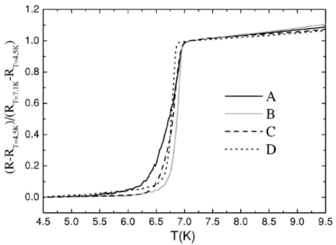
Figure 21: $R(T)$ dependence for four Pb nanowires (A) - (D) with diameters 40, 55, 55 and 70 nm, correspondingly. The transition is broader for narrower wires Piraux Pb nanowire PRB 2004 .

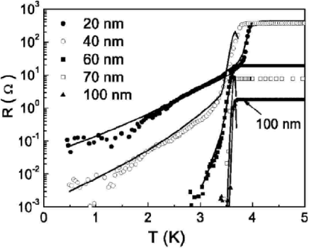
Figure 22: $R(T)$ curves for 20, 40, 60, 70, and 100 nm wide and 6 $\mu$m long Sn nanowire arrays containing respectively 18, 1, 8, 15 and 53 wires in the bundle. The solid lines for 20, 40 and 60 nm wires are the results based on the TAPS model near $T_{C}$ and QPS model below $T_{C}$ Tian Sn nanowire PRB 2005 .

Experiments with Zn nanowires Tian Zn nanowire PRL 2005 ; Tian Zn nanowire PRB 2006 ; Tian specific heat Zn nanowire PRL 2007 lead to observations of unexpected “antiproximity” effect. The shape of the supeconducting transition $R(T)$ of a bundle of Zn nanowires with length up to few $\mu$m depends on the material of the electrodes. It was found that superconductivity is completely or partially suppressed in samples with superconducting electrodes, while clear superconducting transition has been observed in systems with normal electrodes. The origin of the phenomenon is not yet clear, while a model has been proposed Antiproximity theory Clarke PRL 2006 .

Experiments with individual Pb nanowires grown using nanopore electrochemical method show clear superconducting transitions, which get broadened with reduction of the sample diameter (Fig. 21). Unfortunately no theory fits was provided by the authors, while the linear scale of the reported $R(T)$ dependencies complicates an independent quantitative comparison Piraux Pb nanowire PRB 2004 .

Experiments on bundles of several Sn nanowires show clear broadening of the $R(T)$ transitions in the narrowest samples (Fig. 22), which was associated with QPS effects Tian Sn nanowire PRB 2005 . As the number of wires in the measured bundle is not known precisely, quantitative comparison with theoretical predictions appears complicated. In addition, the experiments were presumably performed outside the linear regime: Only rather high dc excitation current densities $j_{bias}\sim$ 10⁴ A/cm² were used being just slightly below the experimentally measured critical current density at low $T$, $j_{C}(T\ll T_{C})\sim$ 10⁵ A/cm².

An advanced method of nanowire fabrication uses MBE grown InP layer on a cleaved In_xGa_1-xAs/InP substrate as a support for thermally evaporated metal (Fig. 23). The applicability of the approach was demonstrated on AuPd and Al Altomare AuPd and Al nanowire fabrication APL 2005 ; Altomare AuPd and Al nanowire fabrication cond-mat 2007 . The method allows fabrication of very long (up to 100 $\mu$m) superconducting (Al) nanowires with effective diameters down to 7 nm. The approach enables pseudo-4-terminal measurements (Fig. 24). The observed broad $R(T)$ dependencies were associated with QPS. Though rather scarce experimental data make quantitative conclusions on the QPS mechanism difficult, the experiments on long Al nanowires Altomare Al nanowire PRL 2006 ; Altomare Al nanowire cond-mat-2005 have a clear message: No correlations between the total normal state wire resistance $R_{N}$ (compared to the quantum resistance unit $R_{q}\simeq 6.45$ k$\Omega$) and superconductivity in such wires was found.

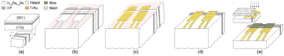
Figure 23: Schematics of the sample fabrication. (a) The sample is cleaved in small strips which are cut in half and glued together with the two (001) plane facing each other, (b) PMMA is spun on the (1$\overline{1}$0) crystallographic plane of the two pieces and a pattern is written using standard EBL and then developed, (c) thermal evaporation is used to deposit a film of Ti/Au (the portion of the film deposited on the PMMA is not shown) and then the two halves are separated, (d) after lift-off and oxygen plasma etching, wet etching is used to define the InP ridge, (e) the wire is formed through the final evaporation appropriately masking the substrate of the sample (top: side view of the evaporation arrangement, bottom: final result) Altomare AuPd and Al nanowire fabrication APL 2005 .

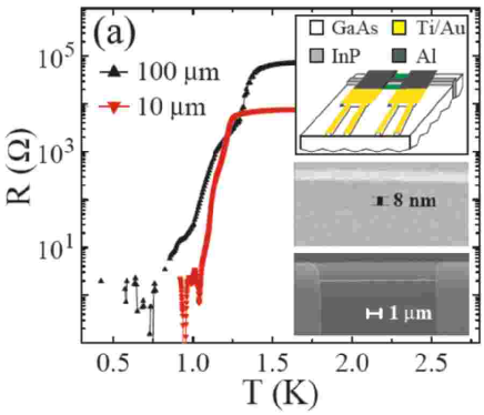
Figure 24: $R(T)$ dependencies for Al nanowires. At temperatures $\lesssim$1 K, samples s2 100 $\mu$m long, $R_{N}$ =86 k$\Omega$ ($\blacktriangle$) and s1: 10 $\mu$m long, $R_{N}$ = 8.3 k$\Omega$ ($\blacktriangledown$) became superconducting. The insets show SEM images and schematic of a typical device containing a 10 $\mu$m long, nominally 8 nm wide Al nanowire (similar to samples s1 and s2): the Al layer does not entirely cover the Au/Ti pads which were measured in series with the superconducting wire (in the main panel this series resistance has been subtracted) Altomare Al nanowire cond-mat-2005 .

A convenient material to study the phenomena associated with phase slips is aluminum. Its bulk critical temperature $T_{C}^{bulk}\sim 1.2$ K is relatively low (see Table I), hence, the QPS rate should be comparatively high enabling pronounced manifestation of fluctuation effects. An additional useful feature of aluminum is its peculiar size dependence of $T_{C}$. Although the origin of this effect remains unclear, an increase of $T_{C}$ with reduction of the characteristic dimension of aluminum structures (wire diameter or film thickness) is a well-known experimental fact and can be taken as granted Shanenko Tc(size) PRB 2006 . This effect does not allow to interpret broadening of $R(T)$ dependencies at temperatures $T<T_{C}^{bulk}$ in terms of sample inhomogeneities, such as constrictions.

Aluminium was chosen for investigations of 1D superconductivity in Refs. Zgirski NanoLett 2005 ; Zgirski QPS PRB 2008 . It was demonstrated that low energy $Ar^{+}$ ion sputtering can progressively and non-destructively reduce dimensions of various nanostructures including nanowires Savolainen IBE method APA 2004 ; Zgirski IBE method Nanotechnology 2008 . The penetration depth of $Ar^{+}$ ions into Al matrix at acceleration voltages of $\sim$ 500 eV is about 2 nm and is comparable to the thickness of naturally formed oxide. The accuracy of the effective diameter determination from the normal state resistance by SEM and SPM measurements is about $\pm$ 2 nm. Only those samples which showed no obvious geometrical imperfections were used for further experiments. To a large extend the method allows one to study the evolution of the size phenomenon, eliminating artifacts related to uniqueness of samples fabricated in independent processing runs. The ion beam treatment polishes the surface of the samples removing inevitable roughness just after fabrication Zgirski IBE method Nanotechnology 2008 (Fig. 25). If there were no detectable geometrical imperfections in the original (thick) wires, they could not be introduced in the course of diameter reduction by low energy ion sputtering.

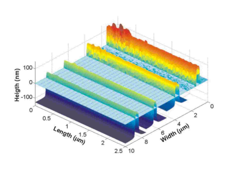
Figure 25: SPM images showing evolution of the shape of the same aluminium nanowire after several sessions of ion beam sputtering. Bright color above the horizonatal plane (initial level of the substrate) corresponds to metal, dark color below indicates sputtered Si substrate. Note the reduction of the initial surface roughness of the nanowire Zgirski QPS PRB 2008 .

After a sequence of sputterings (alternated with $R(T)$ measurements) the wire diameter was reduced from $\sqrt{s}\sim 100$ nm down to $\sqrt{s}$ $\lesssim$ 10 nm. Experiments were performed on several sets of aluminum nanowires with length $X$ equal to 1, 5 and 10 $\mu$m. For larger diameters $\sqrt{s}\gtrsim$ 20 nm the shape of the $R(T)$ dependence is rather ”sharp” and can be qualitatively described by the TAPS mechanism. Note that the abovementioned size dependent variation of $T_{C}$ in aluminum nanowires results in broadening of the $R(T)$ transition and significantly reduces applicability of the TAPS model Zgirski inhomogeneity PRB (Fig. 4). When the wire diameter is further reduced, deviations from the TAPS behavior become obvious (Fig. 26). Fits to the TAPS model fail to provide any reasonable quantitative agreement with experiment for diameter values below $s^{1/2}\leq$ 20 nm even if one hypothetically assumes the existence of unrealistically narrow constrictions not observed by SPM. And, as we already discussed, broadening of the $R(T)$ dependencies in aluminum nanowires at $T<T_{C}^{bulk}$ can hardly be ascribed to geometrical imperfections, such as constrictions. We conclude that the most natural interpretation of our observations is associated with quantum fluctuations.

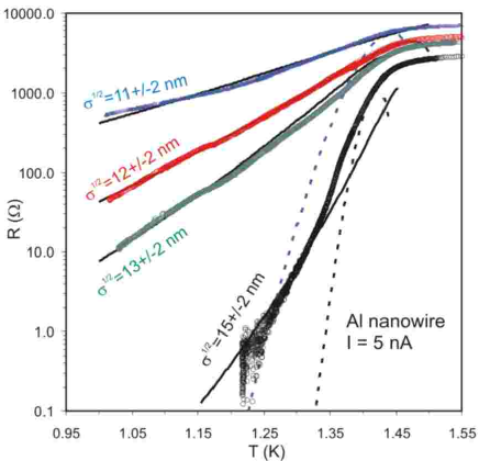
Figure 26: $R(T)$ curves for the thinnest samples obtained by progressive diameter reduction for the same aluminium nanowire with length $X$ = 10 $\mu m$. The TAPS model fitting is shown with dashed lines for 11 and 15 nm samples with the best fit mean free path $l=$ 3 and 10 nm, correspondingly, $T_{C}=$ 1.46 K and critical magnetic field $B_{c}(0)=$ 10 mT. Fits to eq. (161) are shown by solid lines. For 11, 12, 13 and 15 nm wires the fit parameters are: $A\simeq 0.1$; $T_{c}$: 1.64 K, 1.52 K, 1.47 K, and 1.47 K; mean free path $l$ : 7.5 nm, 8.2 nm, 9.5 nm and 9.5 nm; normal state resistance $R_{N}$ : 7200 k$\Omega$, 5300 k$\Omega$, 4200 k$\Omega$ and 2700 k$\Omega$ Zgirski QPS PRB 2008 .

Let us now perform a detailed comparison of the data with theoretical predictions ZGOZ ; ZGOZ2 ; GZ01 discussed in Chapter 5. To begin with, we should select a proper formula for the current-voltage characteristics of the wire which can be applied to the samples Zgirski QPS PRB 2008 . One can employ the general formula (154) derived for sufficiently long wires. It remains not completely clear if this assumption is well satisfied for the wires used in experiments Zgirski QPS PRB 2008 , though it appears that at least the longest wires with $X=10$ $\mu$m are already in this regime ($X/\xi\gtrsim 100$ in this case). In addition, one can recall that in the experimental temperature range not far from $T_{C}$ there can still be sufficiently many quasiparticles above the gap which can produce additional dissipation. Although it would not be fully justified to use eq. (157) in this case, still dissipation can result in additional inter-QPS interaction which can slightly modify the power-law dependencies (155), (156).

Fortunately, this effect, even if exists, does not change our fitting procedure. In order to describe the QPS contribution to the wire resistance we will use the formula

$$R(T)=b_{2}\frac{\Delta_{0}(T)S_{\mathrm{core}}^{2}X}{\xi(T)}\exp(-2S_{\mathrm{core}})T^{\kappa},$$ (164)

while for the non-linear (current-dependent) wire resistance we will use

$$R(I)\propto I^{\kappa}.$$ (165)

Here $b_{2}$ is an unimportant constant which remains the same for all samples. Let us again remind the reader that the dependence $R\propto y^{2}$ comes from pairs of QPS events. As we already discussed, the fugacity (146) depends on temperature via $S_{\mathrm{core}}\propto\Delta_{0}^{1/2}(T)$. An additional power-law dependence enters because of inter-QPS interaction. The parameter $\kappa$ can be equal to $\kappa=2\mu-3$ (as in eqs. (155), (156)) or take somewhat different values due to dissipative contribution. Below we will just use it as a fit parameter instead of the parameter $\mu$.

We first determine this parameter by fitting the $I-V$ curves at a given temperature to the dependence (165), see Fig. 27. From these fits we obtain the values for parameter $\kappa$ (and, correspondingly, for $\mu$) for each sample. Now we perform the fits of the resistance data $R(T)$ taken in the linear regime $I<I_{0}=k_{B}T_{C}/\Phi_{0}\ll I_{c}$ to the dependence (164). There are four parameters to specify for our fits: critical temperature $T_{C}$, normal state resistance $R_{N}$, electron elastic mean free path $l$ (used to re-calculate the dirty limit coherence length $\xi=0.85(\xi_{0}l)^{1/2}$ ), and the numerical factor $A$ of order unity. The critical temperature and the normal state resistance can be trivially deduced from the experimental data for $R(T)$. The electron mean free path $l$ can be roughly estimated from the normal state resistivity $\rho_{N}$ as the product $\rho_{N}l=5\times 10^{-16}\Omega$m² is a well-tabulated value for dirty aluminum. Since the cross section for ultra-narrow nanowires is known from SPM measurements within $\pm$ 2 nm accuracy, there remains a certain room to choose particular values of the mean free path. As a rule of thumb, for all Al nanowires with effective diameter $\sqrt{s}\lesssim$ 20 nm the best-fitted mean free path (at low temperatures) was found to be roughly equal to one-half of the diameter (Fig. 26, caption). This estimate appears quite reasonable taking into consideration that at these scales and temperatures electron scattering occurs merely at the sample boundaries.

Our experimental data and the fits to the theoretical dependence are presented in Fig. 26. We observe that as the sample diameter decreases the $R(T)$ curves become progressively broader, exactly as it is predicted by the QPS theory. Our fits demonstrate a good agreement between theory and experiment, thus confirming the important role of QPS effects in our thinnest wires. For all aluminum nanowires the best-fit value for the parameter $A$ was determined to be $A\simeq 0.1$. This value is smaller than that extracted from the fits to the experimental data by Lau et al. Lau MoGe PRL . We believe that this difference can be attributed to different geometry and degree of inhomogeneity of samples used in these two experiments.

We also point out that the temperature dependence of all fitted curves $R(T)$ is merely determined by that of the QPS action $S_{\mathrm{core}}\propto\Delta_{0}^{1/2}(T)$ which enters the exponent in the expression for the QPS fugacity (146) whereas an additional power-law dependence $\propto T^{\kappa}$ turns out to be insignificant: The fits remain essentially unchanged if we set $\kappa\rightarrow 0$. This is quite natural since $S_{\mathrm{core}}\gg\kappa$ and, on top of that, the temperature dependence of $S_{\mathrm{core}}(T)$ dominates over that emerging from QPS interaction in the temperature interval under consideration.

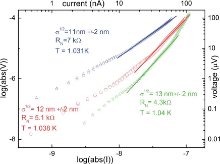
Figure 27: $V(I)$ dependencies of the same samples as in Fig. 26 taken at close temperatures stabilized with accuracy $\pm$ 0.1 mK. Solid lines correspond to the dependence $R\sim I^{\kappa}$ with $\kappa\simeq$ 0.58, 1.31 and 1.49 (from top to bottom) Zgirski QPS PRB 2008 .

To complete our discussion of QPS experiments we point out that very recently an additional experimental evidence for quantum phase slip effects in short MoGe wires was reported Bezr08 . In this experiment the superconducting wires were biased by a large current (just slightly below the critical one) in order to decrease an effective potential barrier for QPS. Similarly to macroscopic quantum tunneling experiments (see, e.g., Ref. Lukens and further references therein) the contribution of the QPS mechanism was identified in Ref. Bezr08 by observing low temperature broadening of the distribution for switching currents at which the nanowire is driven to the normal state by quantum fluctuations of the order parameter. Further quantitative investigations of this effect as well as the analysis of the role of possibly existing external noise and some other extrinsic factors would be highly desirable.

Summarizing our analysis of the experimental data on superconducting nanowires, we can conclude that homogeneity of these wires is one of the central issues which can influence the data interpretation. The methods enabling experiments on the same nanowire while increasing Dynes QPS PRL 1993 ; Dynes QPS and nMR PRL 1997 ; Dynes QPS PRL 1996 or decreasing Zgirski NanoLett 2005 ; Zgirski QPS PRB 2008 its characteristic dimension to a large extent eliminate artifacts related to the uniqueness of samples fabricated in independent processing runs. On the other hand, series of experiments on $MoGe$ wires BT ; Lau MoGe PRL ; Bezryadin MoGe review JPCM 2008 provide large statistics of independent samples. Another conclusion is that longer nanowires appear to be more suitable for experimental investigations of QPS effects while the behavior of very short wires could be to a large extent determined by the Josephson physics (classical or quantum) which can essentially mask the QPS one.

The whole scope of the analyzed experimental data obtained in different groups within different fabrication methods employing different materials clearly demonstrates that at sufficiently low temperatures quantum phase slips provide an important mechanism which may cause non-zero resistance of superconducting nanowires. A vast majority of the data on wires with diameters in the 10 nm range confirms that the TAPS scenario cannot explain the broad $R(T)$ dependencies observed in these structures and favors QPS ZGOZ ; ZGOZ2 ; GZ01 as the only possible scenario. Although in general this scenario can include a number of rather sophisticated physical effects, such as quantum phase transitions (see Chapter 5), it appears that in many cases the rapid change from superconducting to normal behavior can simply be interpreted as a crossover between the regimes of low and high QPS rates GZ01 controlled by the wire cross section $s$ or, equivalently, by the the wire normal state resistance per unit length $R_{N}/X$. Also the dominating contribution to the temperature dependence observed, e.g., in sub-15-nm $MoGe$ BT ; Lau MoGe PRL and aluminium Zgirski QPS PRB 2008 nanowires is well described by that of the QPS rate ZGOZ ; ZGOZ2 ; GZ01 , see Figs. 20 and 26. Although more experiments would be highly desirable, already at this stage we can conclude that the existing experimental data unambiguously confirm our understanding of basic features of QPS physics in superconducting nanowires.

VI.4 Open questions and related topics

VI.4.1 Negative magneotresistance

Application of a weak perpendicular magnetic field to thin superconducting strips governed by fluctuations revealed an unusual effect: negative magnetoresistance (nMR) (Figs. 28 and 29). The phenomenon has been observed in lead Dynes QPS and nMR PRL 1997 and aluminium Zgirski QPS PRB 2008 nanowires. The effect is seen only in very narrow quasi-1D superconducting channels in the resistive state sufficiently far from the critical temperature $T_{C}$. A trivial explanation related to the Kondo mechanism is problematic, as the presence of magnetic impurities in those experiments is believed to be negligible and – in any case – has not been independently proven. Even if we were to assume the presence of Kondo impurities, several features of nMR would still remain unclear. First, the corresponding magnetic fields are too small to polarize magnetic moments of any impurities at such values of $T$. In addition, it is known that aluminum is immune to creation of localized magnetic moments with concentration up to few at % Magnetic ions in Al Jalkanen SolStComm 2007 . Second, there is a pronounced diameter dependence, making nMR observable only in thinnest wires. Third, the onset of superconductivity is not affected by weak magnetic fields: nMR is observed only at the bottom part of the $R(T)$ transition. Perhaps we should also mention another effect – enhancement of the critical current by magnetic field – which was observed in MoGe and Nb nanowires Bezryadin nMR MoGe and Nb PRL 2006 and attributed to interplay between spin-exchange scattering from residual magnetic impurities and the orbital and Zeeman effects Bezryadin nMR theory EPL 2006 . However, it remains unclear if this effect is related to nMR in any way. On top of that, presently there exists no evidence for the presence of magnetic impurities in experiments with aluminium Zgirski QPS PRB 2008 and lead Dynes QPS and nMR PRL 1997 .

Figure 28: (a) Resistive transitions in zero magnetic field for 58 nm wide lead wires of different thicknesses. Superconductivity is suppressed with reduction of the wire thickness. The symbols represent the points at which the magnetoresistance was measured. (b)–(e) Magnetoresistance for the wire at different thicknesses. The numbers indicate the temperature in Kelvin Dynes QPS and nMR PRL 1997 .

Figure 29: Slowly ($\sim$1 h) recorded dependence $R(T,B_{ext}=const)$ for the 11-nm sample from Fig. 26. The perpendicular magnetic field $B_{ext}=$19.6 mT was switched on and off several times while sweeping the temperature. The top branch corresponds to zero field, while the lower one to the field “on”. Inset: resistance versus perpendicular magnetic field $R(B_{ext},T=const)$ for the same sample measured at constant temperature and small ac current Zgirski QPS PRB 2008 .

NMR has been observed in tin microbridges Kadin pair breaking JLTP 1978 and aluminium nanostructures demonstrating the resistive transition anomaly (see below) Santhanam nMR anomaly . However, the dimensions of those structures were significantly larger as compared to ultrathin nanowires Dynes QPS and nMR PRL 1997 ; Zgirski QPS PRB 2008 . Presumably the origin of nMR in these earlier reports can be ascribed to charge imbalance Kadin pair breaking JLTP 1978 or to sample inhomogeneity Arutyunov R(T) anomaly PRB 1999 . NMR has been predicted in disordered superconducting wires PA . However, the contribution responsible for nMR within this model is exponentially small as compared to the effective resistance produced by TAPS. This is clearly not the case in experiments Dynes QPS and nMR PRL 1997 ; Zgirski QPS PRB 2008 .

A plausible explanation of the nMR effect could be related to the reduction of the energy gap $\Delta_{0}$ in the magnetic field. It was argued ZGOZ2 that this reduction leads to the following trade-off. On one hand, the core action $S_{\mathrm{core}}\propto\Delta_{0}^{1/2}$ decreases with increasing magnetic field and, hence, the QPS rate becomes bigger. On the other hand, the quasiparticle resistance $R_{qp}\propto\exp(\Delta_{0}/T)$ decreases too implying increasing dissipation which, in turn, suppresses the QPS rate. Provided the latter trend dominates over the former one, the contribution of quantum fluctuations to the wire resistance gets reduced with increasing magnetic field, thus leading to nMR ZGOZ2 . Yet another idea employs possible formation of a charge imbalance region accompanying each phase slip event Arutyunov nMR Physica C 2008 . This non-equilibrium region, if it exists, would provide dissipation outside the core of a phase slip. The corresponding Ohmic contribution can be effectively suppressed by the magnetic field, resulting in nMR. However, so far the validity of the charge imbalance concept was only demonstrated at temperatures sufficiently close to $T_{C}$ and its applicability to QPS is by no means obvious. This mechanism still requires a solid theoretical justification.

VI.4.2 Step-like R(T) dependencies in crystalline 1D structures

Rather unusual step-like shape of $R(T)$ transition has been reported in tin whiskers R(T) steps Webb-Warburton PRL 1968 . In relatively long structures $X\sim 0.8$ mm with ”manually” fixed electrodes using conducting epoxy and/or Wood metal Meyer RT steps the steps were observed at relatively high measuring current densities $j\sim 10^{4}$ A/cm² (Fig. 30). In hybrid whisker-based structures with lithographically-fabricated electrodes Arutyunov SOG whiskers (Fig. 6) the steps on $R(T)$ dependencies were observed between closely located probes ($X<$ 10 $\mu$m) and at current densities as low as $j\sim 10^{2}$ A/cm² (Fig. 31). For comparison, the experimental critical current density in pure tin whiskers at sufficiently small temperatures reaches its theoretical value $j_{c}(0)\sim 10^{7}$ A/cm². The origin of the phenomenon is not clear. The step-like $R(T)$ dependencies were not reported in similar experiments using tin whiskers Webb R(T) in Sn whiskers ; Tinkham R(T) in Sn whiskers . Note that the steps on $R(T)$ transition should not be confused with step-like $I-V$ characteristics observed in 1D superconducting wires very close to the critical temperature and at bias currents exceeding the temperature-dependent critical value $I>I_{C}(T)$. The origin of the $I-V$ steps is usually associated with current-induced non-equilibrium effects Tidecks ; Kopnin book .

Figure 30: Step-like $V(T)$ dependence in tin whisker at various excitation currents Meyer RT steps .

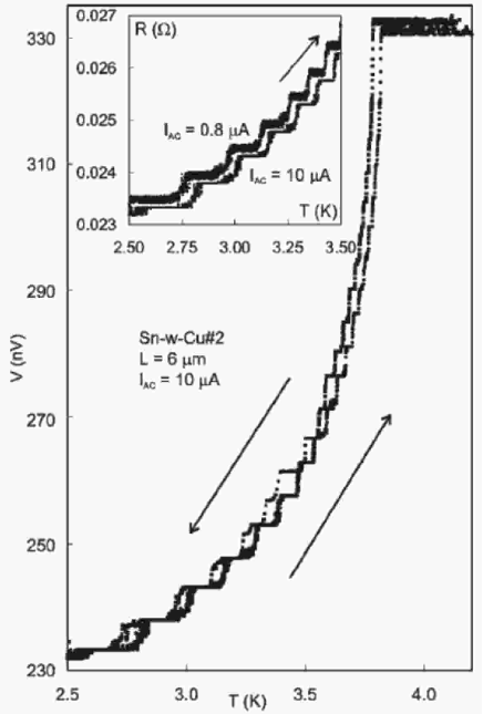
Figure 31: An example of a pronounced step-like $V(T)$ dependence in a hybrid whisker-based structure similar to that of Fig. 6. Arrows indicate the direction of the temperature sweep. Small hysteresis is a consequence of the temperature measurement finite response time. The inset shows an enlarged view of several $R(T)$ steps measured at two different currents. The curves are shifted slightly due to zero offset drift of the front-end battery powered preamplifier Arutyunov SOG whiskers .

VI.4.3 Resistive transition anomaly

Intensive studies of various lift-off fabricated quasi-1D nanostructures revealed an unusual ”resistive transition anomaly”: Resistance increase above the normal state value $R_{N}$ at the top of the superconducting transition  (Fig. 32) Santhanam R(T) anomaly ; Moschalkov Little-Parks anomaly ; Moshchalkov R(T) anomaly ; Arutyunov R(T) anomaly PRB 1999 ; Kim R(T) anomaly Physica B 1994 ; Kwong R(T) anomaly PRB 1991 ; Park R(T) anomaly PRL 1995 ; Strunk R(T) anomaly PRB 1996 ; Strunk R(T) anomaly Superlat 1996 ; Strunk R(T) anomaly JAP 1998 ; Strunk R(T) anomaly PRB 1998 . No special correlation has been observed between the absolute value of the sample length $X$ (distance between the probes) and the magnitude of the anomaly. Pronounced ”bumps” were observed only in relatively short structures with width $w$ $\gtrsim X/10$. No dependence upon the film thickness within the range 30–90 nm has been noticed either. The same statement holds for the sample topology: both single-connected and non-single-connected structures displayed the bumps. For the same multiterminal structure, the anomaly could be clearly observed for a pair of voltage contacts, while the neighboring segment showed no signs of the effect. For a given set of contacts, the magnitude of the resistive anomaly sometimes depends on the cooling history. Heating up to $\sim$50 K could eliminate the effect. Variation of the measuring current or application of the magnetic field can modify the magnitude of the bump (Fig. 33).

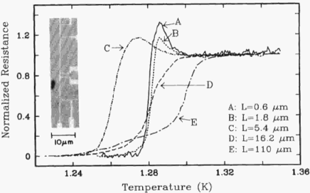
Figure 32: Normalized resistance as a function of temperature for five aluminium samples A-E showing the resistance anomaly. Longer wires display a smaller and broader peak. Inset: The sample configuration for three shortest wires Santhanam R(T) anomaly .

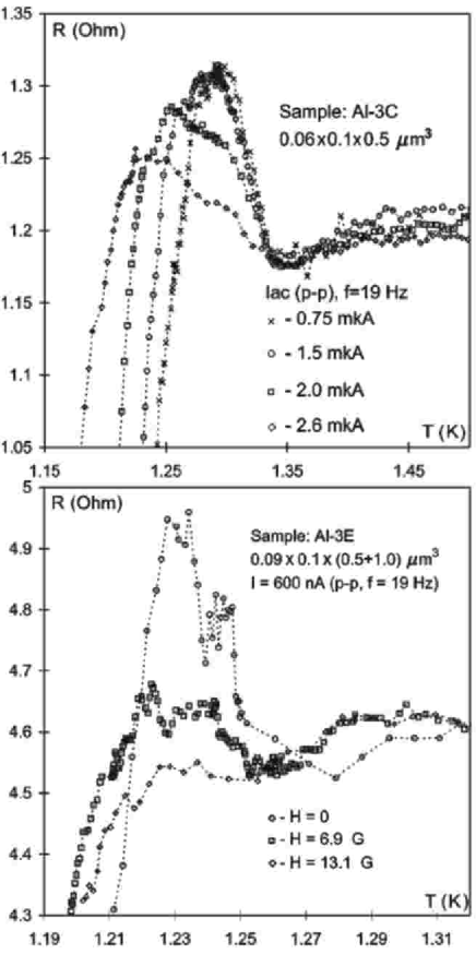
Figure 33: Top part of the resistive transition $R(T)$ for aluminium multiterminal nanostructure at different measuring ac currents (top) and at various external magnetic fields normal to the sample surface (bottom) Arutyunov R(T) anomaly PRB 1999 .

Let us point out that experimentalists frequently use lock-in technique in order to increase the signal-to-noise ratio. Should a dc component occasionally occur (e.g., due to improper grounding), experimental dependencies could become proportional to $dV/dI(T)$ rather than to the desired $R(T)\equiv V_{ac}/I_{ac}$ resulting in ”veird”-looking $R(T)$ curves. Utilization of rf filters, such as widely used commercial $\pi$-filters, can also contribute to non-monotonous $R(T)$ transitions due to re-arrangement of the measuring ac current through the ground loop even at rather low frequencies $\sim$10 Hz.

Various physical reasons for the resistive transition anomaly in superconducting nanostructures have been proposed, such as the fluctuation-governed resistive state Moschalkov R(T) anomaly PRB 1994 ; Moschalkov R(T) anomaly PRB 1997 ; Arutyunov R(T) anomaly PRB 1996 nonequilibrium quasiparticle charge imbalance within the locus of N/S boundary Kwong R(T) anomaly PRB 1991 ; Park R(T) anomaly PRL 1995 or phase-slip centers Santhanam R(T) anomaly ; Arutyunov R(T) anomaly PRB 1996 . It should be noted that the resistive transition anomaly has only been reported in relatively inhomogeneous lift-off fabricated nanostructures with the width of the $R(T)$ transition strongly exceeding that predicted by the fluctuation models. It has been shown that the phenomenon can be qualitatively explained by simple geometric considerations concerning the shape of the N/S phase boundary of an inhomogeneous wire in the resistive state Landau R(T) anomaly PRB 1997 . The approach has been extended Arutyunov R(T) anomaly PRB 1999 demonstrating that the combination of the two effects provides reasonable agreement with experiments: (i) a geometry effect of the formation of non-perpendicular (to the wire axis) N/S boundaries and the corresponding rearrangement of current across the wire, and (ii) the existence of nonzero and strongly anisotropic effective resistance of the nonequilibrium superconducting region close to the N/S interface. Considered separately, neither of these two contributions could provide quantitative agreement with the experimental data.

To summarize, it is possible that the resistive transition anomaly originates from “dirty physics” related to inhomogeneity of the finite length lift-off fabricated wires. This is supported by the fact that no signs of the anomaly were reported in pure 1D systems Webb R(T) in Sn whiskers ; Tinkham R(T) in Sn whiskers ; Meyer RT steps ; Arutyunov SOG whiskers .

VI.4.4 $T_{C}$ dependence on wire diameter.

Since early days of low-dimensional superconductivity it is known that the critical temperature of thin films $T_{C}^{2D}$ and wires $T_{C}^{1D}$ differ from the corresponding bulk value $T_{c}^{bulk}$. In indium, aluminum and zink nanowires $T_{C}$ increases with decreasing the characteristic dimension Giordano QPS PRL 1988 ; Altomare Al nanowire PRL 2006 ; Zgirski NanoLett 2005 ; Tian Zn nanowire PRL 2005 . In lead, niobium and MoGe an opposite tendency has been observed Dynes QPS PRL 1993 ; Bezryadin Nb nanowires ; Bezryadin MoGe and Nb wires ; BT ; Bezryadin MoGe TAPS EPL-2006 . No noticeable variations of $T_{C}$ have been reported in tin nanowires Tian Sn nanowire APL 2003 ; Tian Sn nanowire PRB 2005 ; Piraux Sn nanowire APl 2004 ; Piraux Sn nanowire NanoSci NanoTech 2005 .

The early models considered size-dependent modification of the electron-phonon spectrum and found the corresponding variation of the critical temperature of thin films Tc(size) theory McMillan PR 1968 ; Tc(size) theory Garland PRL 1968 ; Tc(size) Allen PR69 . However, later it was noticed that the phonon spectrum renormalization can significantly contribute to variations of $T_{C}$ only in ultra-thin structures, while experimentally the effect is observed also in rather thick films (e.g. up to $t\sim 50$ nm in the case of aluminum), where the phonon spectrum is almost identical to that of bulk samples. Additionally, it was found that the critical temperature $T_{C}^{2D}$ of ultra-thin quench-condensed films depends not only on thickness, but also on annealing made in situ in the measuring chamber at cryogenic temperatures Tc(size) experiment Ga Parshin PRB 1996 , indicating that the morphology of the film is also important. Another significant effect is an interplay between disorder and electron-electron interactions which can lead to substantial suppression of $T_{C}$ in reduced dimensions Fin . On the other hand, the so-called shape resonance effect Tc(size) theory Shanenko PRB 2006 ; Shanenko Tc(size) PRB 2006 can be responsible for the enhancement of $T_{C}$. To conclude, after years of intensive experimental and theoretical studies, the origin of the size dependence of the critical temperature $T_{C}$ remains not fully understood and in many cases it can be determined by a number of different factors.

VII Persistent currents in superconducting nanorings

VII.1 Persistent currents and quantum phase slips

It is well known that superconducting rings pierced by external magnetic flux $\Phi_{x}$ develop circulating persistent currents (PC) which never vanish. This phenomenon is a fundamental consequence of macroscopic phase coherence of Cooper pair wave functions. In the case of bulk metallic rings fluctuations of the phase $\varphi$ of the order parameter can be neglected, i.e. $\varphi$ can be considered as a purely classical variable. In this case the total phase difference $\varphi(X)-\varphi(0)$ accumulated along the ring circumference $X=2\pi R$ is linked to the external flux $\Phi_{x}$ inside the ring by the well known relation

$$\varphi(X)-\varphi(0)=2\pi p+\phi_{x},$$ (166)

where $p$ is an integer number, $\phi_{x}=\Phi_{x}/\Phi_{0}$ and, as before, $\Phi_{0}$ is the superconducting flux quantum. This relation implies the existence of a phase gradient along the ring which, in turn, means the presence of discrete set of current and energy states labelled by the number $p$. At sufficiently low temperatures $T\ll\Delta_{0}$ quasiparticles are practically irrelevant and the grand partition function of the ring takes the form

$${\mathcal{Z}}_{\phi_{x}}=\sum_{p=-\infty}^{\infty}\exp(-E_{p}(\phi_{x})/T),$$ (167)

where

$$E_{p}(\phi_{x})=\frac{E_{R}}{2}(p+\phi_{x})^{2},\quad E_{R}=\frac{\pi^{2}\hbar^{2}N_{0}D\Delta_{0}s}{R}$$ (168)

defines flux-dependent energy states of a diffusive superconducting ring with radius $R$ and cross-section $s$. The ground state energy $E(\phi_{x})=$min${}_{p}E_{p}(\phi_{x})$ is a periodic function of the flux $\Phi_{x}$ with the period $\Phi_{0}$. The derivative of the ground state energy with respect to the flux defines the persistent current

$$I(\Phi_{x})=c\left(\frac{\partial E(\Phi_{x})}{\partial\Phi_{x}}\right).$$ (169)

Combining eqs. (168) and (169) one finds

$$I=2\pi emv_{s}N_{0}D\Delta_{0}s,$$ (170)

where $m$ is the electron mass and

$$v_{s}(\phi_{x})=\frac{\hbar}{2mR}\mathrm{min}_{p}\left(p+\frac{\Phi_{x}}{\Phi_{0}}\right)$$ (171)

is the superconducting velocity. Both the current $I$ and the velocity $v_{s}$ are periodic functions of the magnetic flux $\Phi_{x}$ showing the familiar sawtooth behavior, see also Fig. 34.

Figure 34: The energy (a) and persistent current (b) for a superconducting nanoring as functions of magnetic flux without fluctuations, with weak and with strong QPS effects shown respectively by solid, dashed and dotted lines MLG .

This picture remains applicable as long as fluctuations of the superconducting phase $\varphi$ can be neglected, i.e. as long as the ring remains sufficiently thick. Upon decreasing the thickness of a superconducting wire $\sqrt{s}$ down to values $\sim 10$ nm range one eventually reaches the new regime in which quantum fluctuations of the phase gain importance and, as it will be demonstrated below, essentially modify the low temperature behavior of superconducting nanorings.

As we have already learned, at low $T$ the most important fluctuations in superconducting nanowires are quantum phase slips. Each phase slip event implies transfer of one flux quantum $\Phi_{0}$ through the wire out of or into the ring and, hence, yields the change of the total flux inside the ring by exactly the same amount. In other words, each QPS yields a jump between two neighboring energy states $E_{p}$ (168) (i.e. between two neighboring parabolas in Fig. 34). As a result of such jumps the flux inside the ring fluctuates, its average value $\langle\Phi(\Phi_{x})\rangle$ decreases and so does the persistent current $I$. One can also anticipate that the magnitude of this effect should increase with the ring perimeter $X$. This is because the QPS rate $\gamma_{QPS}$ increases linearly with $X$, i.e. the bigger the ring perimeter the higher the probability for QPS to occur anywhere along the ring.

A quantitative theory of QPS effects in nanorings was proposed by Matveev et al. MLG . These authors employed a model of a closed chain of Josephson junctions in which case QPS can occur only across such junctions. Here will extend our theory of QPS (Chapter 5) and analyze the effect of quantum fluctuations on persistent currents in uniform superconducting nanorings. The key conclusions remain the same for both models.

Before turning to technical details it is instructive to point out a formal equivalence between the phenomenon discussed here and charging effects in ultrasmall Josephson junctions (or Cooper pair boxes) sz . Indeed, the energy states of our ring (168) driven by the (normalized) external magnetic flux $\phi_{x}$ (see Fig. 34) are fully analogous to such states of a capacitor in a Cooper pair box driven by the (normalized) gate charge $Q_{x}/2e$. Furthermore, we will demonstrate that there exists a direct analogy between QPS events changing the flux inside the ring by $\Phi_{0}$ and tunneling events of single Cooper pairs changing the capacitor charge by $2e$. This equivalence is reminiscent of the well known duality between phase and charge representations sz and will be exploited in our consideration.

We start from the case of sufficiently thick superconducting rings where QPS effects can be neglected. In this case by virtue of Poisson’s resummation theorem (see, e.g., Sec. 3.3.2 in Ref. sz ) one can identically transform the ring partition function (167) to the following expression

$${\mathcal{Z}}_{\phi_{x}}=\sum_{k=-\infty}^{\infty}\exp(i2\pi k\phi_{x})\int d\theta_{0}\int_{\theta_{0}}^{\theta_{0}+2\pi k}{\mathcal{D}}\theta\exp(-S_{0}[\theta]),$$ (172)

where

$$S_{0}[\theta]=\int_{0}^{\beta}d\tau\frac{1}{2E_{R}}\left(\frac{\partial\theta}{\partial\tau}\right)^{2}$$ (173)

and $1/E_{R}$ plays the role of a ”mass” for a ”particle” with the coordinate $\theta$. This coordinate represents an effective angle. It is formally analogous to the Josephson phase variable in which case $E_{R}$ just coincides with the charging energy.

Let us now consider thinner rings where QPS effects gain importance. In this case we should include all transitions between different energy states (168) labelled by the number $p$. As we already discussed these transitions are just QPS events with the rate $\gamma_{QPS}$ defined in eq. (140). Let us fix $p=0$ and take into account virtual transitions to all other energy states and back. Performing summation over all such contributions we arrive at the series in powers of the rate $\gamma_{QPS}$ (or fugacity $y$) similar to eq. (145). Assuming that both the ring perimeter $X$ and its thickness are not too large (the latter condition restricts the parameter $\mu$) one can neglect weak logarithmic interaction (142) between different phase slips. Then spatial QPS coordinates $x_{n}$ become exact zero modes and can be trivially integrated out. As a result, we arrive at the following contribution to the partition function

$${\tilde{Z}}(\phi_{x})=\int_{\phi_{x}}^{\phi_{x}}{\mathcal{D}}\phi(\tau)\sum_{n=0}^{\infty}\frac{1}{2n!}\left(\frac{\gamma_{QPS}}{2}\right)^{2n}\int_{0}^{\beta}d\tau_{1}...\int_{0}^{\beta}d\tau_{2n}$$

$$\times\sum_{\nu_{i}=\pm 1}\delta(\dot{\phi}(\tau)-\dot{\phi}_{n}(\tau))\exp\left(-\int_{0}^{\beta}d\tau\frac{E_{R}\phi^{2}(\tau)}{2}\right)$$ (174)

where, as before, the summation is carried out over neutral charge configurations (147),

$$\phi_{n}(\tau)=\sum_{j=1}^{n}\nu_{j}\Theta(\tau-\tau_{j})$$ (175)

and $\Theta(\tau)$ is the theta-function. We note that the term in the exponent describes virtual energy changes occurring due to QPS events. What remains is to add up similar contributions from all other parabolas with $p\neq 0$. In this way we arrive at the final expression for the grand partition function of the nanoring

$${\mathcal{Z}}_{\phi_{x}}=\sum_{p=-\infty}^{\infty}{\tilde{Z}}(p+\phi_{x}).$$ (176)

Together with eq. (174) this result fully accounts for all QPS events in our system.

In the absence of QPS (i.e. for $\gamma_{QPS}\to 0$) eqs. (176), (174) obviously reduce to (167). For non-zero $\gamma_{QPS}$ one can rewrite the partition function (174), (176) in the equivalent form of the following path integral

$${\mathcal{Z}}_{\phi_{x}}=\sum_{k=-\infty}^{\infty}\exp(i2\pi k\phi_{x})\int d\theta_{0}\int_{\theta_{0}}^{\theta_{0}+2\pi k}{\mathcal{D}}\theta\exp(-S[\theta]),$$ (177)

where

$$S[\theta]=S_{0}[\theta]-\gamma_{QPS}\int_{0}^{\beta}d\tau\cos\theta(\tau).$$ (178)

In order to demonstrate that the partition function (177), (178) is identical to that defined in eqs. (174), (176) it suffices to perform the Hubbard-Stratonovich transformation of the kinetic term (173) (which amounts to introducing additional path integral over $\phi(\tau)$), to formally expand $\exp(-S[\theta])$ in powers of $\gamma_{QPS}$ and then to integrate out the $\theta$-variable in all terms of these series. After these straightforward steps we arrive back at eqs. (174), (176). We also note that this procedure is described in Sec. 3.3.5 of Ref. sz , therefore we can avoid further details here.

Eqs. (177), (178) define the grand partition function for a quantum particle in a cosine periodic potential which is, in turn, equivalent to that for a Josephson junction in the presence of charging effects sz . This partition function can be identically rewritten as (cf. eq. (3.94) in Ref. sz )

$${\mathcal{Z}}_{\phi_{x}}=\sum_{p=-\infty}^{\infty}\exp(-\tilde{E}_{p}(\phi_{x})/T),$$ (179)

where $\tilde{E}_{p}(\phi_{x})$ are the energy bands of the problem defined by the solutions of the well-known Mathieu equation. For $\gamma_{QPS}\ll E_{R}$ one has

$$\tilde{E}_{0}(\phi)=\frac{E_{R}}{2\pi^{2}}\arcsin^{2}\left[\left(1-\frac{\pi^{2}}{2}\left(\frac{\gamma_{QPS}}{E_{R}}\right)^{2}\right)\sin(\pi\phi_{x})\right],$$ (180)

i.e. the energy bands remain nearly parabolic $\tilde{E}_{p}(\phi)\sim E_{p}(\phi)$ except in the vicinity of the crossing points where gaps open due to level repulsion (see Fig. 34). In this limit the value of the gap between the lowest and the first excited energy bands just coincides with the QPS rate $\delta E_{01}=\gamma_{QPS}$. For larger $\gamma_{QPS}$ the bandwidth shrinks while the gaps become bigger. In the limit $\gamma_{QPS}\gg E_{R}$ the lowest band coincides with

$$\tilde{E}_{0}(\phi)=\frac{8}{\sqrt{\pi}}\gamma_{QPS}^{3/4}(E_{R})^{1/4}e^{-8\sqrt{\gamma_{QPS}/E_{R}}}(1-\cos(2\pi\phi_{x})).$$ (181)

The gap between the two lowest bands is $\delta E_{01}=\sqrt{\gamma_{QPS}E_{R}}$.

These results are sufficient to evaluate PC in superconducting nanorings in the presence of quantum phase slips. As before, taking the derivative of the ground state energy with respect to the flux $\Phi_{x}$ and making use of eq. (140) we find that for $\gamma_{QPS}\ll E_{R}$ and outside immediate vicinity of the points $\phi_{x}=1/2+p$ PC is again defined by eqs. (170), (171). In the opposite limit $\gamma_{QPS}\gg E_{R}$ we find

$$I = \tilde{I}_{0}\sin(2\pi\phi_{x}),$$

$$\tilde{I}_{0} = \frac{16e}{\sqrt{\pi\hbar}}\gamma_{QPS}^{3/4}(E_{R})^{1/4}e^{-8\sqrt{\gamma_{QPS}/E_{R}}}.$$ (182)

We observe that in the latter limit PC is exponentially suppressed as

$$\tilde{I}_{0}\propto\exp(-R/R_{c}),$$ (183)

where neglecting a numerical prefactor we estimate

$$R_{c}\sim\xi\exp(S_{\mathrm{core}}/2).$$ (184)

This simple formula sets the size scale beyond which one would expect PC to be exponentially suppressed in superconducting nanorings with $\sqrt{s}\lesssim 10$ nm. E.g. for $\xi$ of order 100 nm and $S_{\mathrm{core}}\approx 10$ eq. (184) yields $R_{c}$ of order of a micron.

We would like to emphasize that during our analysis we employed only one approximation neglecting logarithmic inter-QPS interaction effects. If needed, such effects can also be included into our consideration and may only lead to unimportant modifications in our results for rings with very large perimeters $X$.

The above results demonstrate practically the same qualitative features as those found within a different approach for the model of nanorings formed by Josephson chains MLG . In particular, both for granular and for homogeneous rings the dependence of PC on $\phi_{x}$ gradually changes from sawtooth to sinusoidal as the ring perimeter $X$ increases. This change is accompanied by suppression of PC amplitude which eventually becomes an exponentially decaying function of the ring radius $R$ (183) in the limit $R>R_{c}$. In other words, eq. (183) sets the length scale $R_{c}$ beyond which persistent currents in superconducting nanorings should be essentially washed out by quantum fluctuations. In some sense the scale $2\pi R_{c}$ plays the role of a dephasing length in our problem demonstrating that zero-point fluctuations can destroy macroscopic phase coherence down to $T\to 0$ even in superconducting systems.

This conclusion is qualitatively consistent with the results derived for normal metallic conductors GZ ; GZ1 ; GZ2 ; GZ98P and single channel rings coupled to dissipative baths GZ98P ; Paco ; Carlos . In fact, a close similarity between the partition function (177), (178) and those studied in Refs. Paco ; Carlos exists on a formal level as well: These problems are described by similar path integrals except in the case of normal rings coupled to dissipative environments one should include the corresponding non-local in time term into the action instead of the last term in eq. (178). At sufficiently large $X$ these path integrals can also be handled in exactly the same manner: In both problems the dominating contribution comes from instantons (kinks) describing quantum tunneling of the angle variable $\theta$ between different topological sectors of the problem. In all cases this procedure yields low temperature PC in the form (182) where one finds $\tilde{I}_{0}\propto\exp(-(X/L_{\varphi})^{2})$ in the case of Caldeira-Leggett environments GZ98P ; Paco ; Carlos and $\tilde{I}_{0}\propto\exp(-X/L_{\varphi})$ in the case of so-called dirty electron gas environments Carlos .

An important qualitative difference between our present problem and those of normal nanorings with dissipation lies in the fact that in the latter case dissipation explicitly violates time-reversal symmetry (thus causing genuine decoherence of electrons), while no such symmetry is violated in eqs. (177), (178). Hence, in our case – in contrast to GZ98P ; Paco ; Carlos – exponential suppression of PC (182) can also be interpreted as a non-trivial coordinate-dependent renormalization effect. This difference is just the same as that between dissipativeless Cooper pair tunneling (which, just like QPS, opens inter-band gaps in the spectrum of Josephson junctions) and dissipative single electron tunneling (which opens no such gaps). For more details on the latter subject we refer the reader to the review sz .

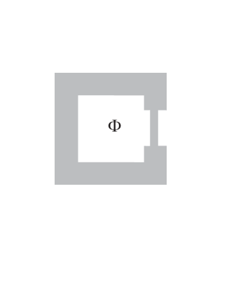
Figure 35: Superconducting ring with a ”quantum phase slip junction”.

Finally we should mention that one can also consider a slightly modified situation of rings consisting of thicker and thinner parts, as it is shown in Fig. 35. Assuming that QPS effects are negligible in a thicker part of the ring and they can only occur in its thinner part (of length $d$) we arrive at exactly the same results as above in which one should only replace the ring perimeter $X$ by the length $d$. In particular, it follows from our analysis that such rings also exhibit the property of an exact duality to mesoscopic Josephson junctions if we identify $E_{R}$ with the junction charging energy $E_{C}$ and the QPS rate $\gamma_{QPS}$ with the Josephson energy $E_{J}$. For this reason Mooij and Nazarov MN suggested to call systems depicted in Fig. 35 ”quantum phase slip junctions” and argued that any known result on electron transport in circuits containing Josephson junctions can be exactly mapped onto a dual result for a QPS junction in a dual circuit. This observation can be used in metrology, e.g., for practical implementation of the electric current standard in the above structures. Mooij and Harmans MH proposed to use rings with QPS junctions for experimental realization of quantum phase slip flux qubits.

It is also worth pointing out that previously a similar exact duality between phase and charge variables in Josephson junctions was discussed AvOd ; Z90 ; sz , see, e.g., eq. (5.76) in Ref. sz . According to this property the Josephson junction itself can also be a QPS junction if we interchange the canonically conjugate phase and (quasi)charge variables $\varphi\to\pi q/e$. In this sense one can identify the angle variable $\theta$ with the (quasi)charge $\pi q/e$ passing through the QPS junction.

VII.2 Parity effect and persistent currents

In our previous analysis of QPS effects in superconducting nanorings we followed the standard technique developed for grand canonical ensembles, i.e. we implicitly assumed that the total number of electrons in the system $N$ may fluctuate and the chemical potential $\tilde{\mu}$ is fixed. Obviously, this assumption is not correct for rings which are disconnected from any external circuit. In that case electrons cannot enter or leave the ring and, hence, the number $N$ is strictly fixed, but the chemical potential $\tilde{\mu}$, on the contrary, fluctuates. It turns out that novel effects emerge in this physical situation. These effects will be discussed below in this section. To a large extent we will follow the analysis developed in Refs. SZ ; KKZ ; Z04 ; SZ2 .

It is well known that thermodynamic properties of isolated superconducting systems are sensitive to the parity of the total number of electrons AN92 ; Tuo93 ; sz94 ; vDZGT even though this number is macroscopically large. This parity effect is a fundamental property of a superconducting ground state described by the condensate of Cooper pairs. The number of electrons in the condensate is necessarily even, hence, for odd $N$ at least one electron remains unpaired having an extra energy equal to the superconducting energy gap $\Delta_{0}$. This effect makes thermodynamic properties of the ground state with even and odd $N$ different. Clear evidence for such parity effect was demonstrated experimentally in small superconducting islands Tuo93 ; Laf93 ; RT .

At the first sight, this parity effect should have little impact on the supercurrent because of the fundamental uncertainty relation $\delta N\delta\varphi\gtrsim 1$. Should the electron number $N$ be fixed, fluctuations of the superconducting phase $\varphi$ become large disrupting the supercurrent. On the other hand, in transport experiments with fluctuations of $\varphi$ being suppressed the parity effect cannot be observed because of large fluctuations of $N$.

Consider now isolated superconducting rings pierced by the magnetic flux $\Phi_{x}$. In accordance with the number-phase uncertainty relation the global superconducting phase of the ring fluctuates strongly in this case, however these fluctuations are decoupled from the supercurrent and therefore cannot influence the latter. In this situation the parity effect may substantially modify PC in superconducting nanorings at sufficiently low temperatures. In particular, we will show that changing the electron parity number from even to odd results in spontaneous supercurrent in the ground state of such rings without any externally applied magnetic flux. In other words, our fundamental conclusion will be that the BCS ground state of a canonical ensemble with odd number of electrons is the state with spontaneous supercurrent.

VII.2.1 Parity projection formalism

In order to systematically investigate interplay between the parity effect and persistent currents in superconducting nanorings we will employ the parity projection formalism SZ ; SZ2 ; JSA94 ; GZ294 ; AN94 which we will briefly outline here.

The grand canonical partition function

$${\mathcal{Z}}(T,\tilde{\mu})=\mathrm{Tr}e^{-\beta({\mathcal{H}}-\tilde{\mu}N)}$$ (185)

is linked to the canonical one $Z(T,N)$ as

$${\mathcal{Z}}(T,\tilde{\mu})=\sum\limits_{N=0}^{\infty}Z(T,N)\exp\biggl{(}{\frac{\tilde{\mu}N}{T}}\biggr{)}.$$ (186)

Here and below ${\mathcal{H}}$ is the system Hamiltonian. Inverting this relation and defining the canonical partition functions $Z_{e}$ and $Z_{o}$ respectively for even ($N\equiv N_{e}$) and odd ($N\equiv N_{o}$) ensembles, one gets

$$Z_{e/o}(T)={\frac{1}{2\pi}}\int_{-\pi}^{\pi}due^{-iN_{e/o}u}{\mathcal{Z}}_{e/o}(T,iTu),$$ (187)

where

$${\mathcal{Z}}_{e/o}(T,\tilde{\mu}) = {\frac{1}{2}}\mathrm{Tr}\left\{\big{[}1\pm(-1)^{N}\big{]}e^{-\beta({\mathcal{H}}-\tilde{\mu}N)}\right\}$$ (188)

$$= {\frac{1}{2}}\left({\mathcal{Z}}(T,\tilde{\mu})\pm{\mathcal{Z}}(T,\tilde{\mu}+i\pi T)\right)$$

are the parity projected grand canonical partition functions. For $N\gg 1$ it is sufficient to evaluate the integral in (187) within the saddle point approximation

$$Z_{e/o}(T)\sim e^{-\beta(\Omega_{e/o}-\tilde{\mu}_{e/o}N_{e/o})},$$ (189)

where ${\Omega}_{e/o}=-T\ln{\mathcal{Z}}_{e/o}(T,\tilde{\mu})$ are the parity projected thermodynamic potentials,

$${\Omega}_{e/o}={\Omega}_{f}-T\ln\bigg{[}\frac{1}{2}\Big{(}1\pm e^{-\beta({\Omega_{b}}-{\Omega_{f}})}\Big{)}\bigg{]}$$

and ${\Omega}_{f/b}=-T\ln\left[\mathrm{Tr}\left\{(\pm 1)^{\mathcal{N}}e^{-\beta({\mathcal{H}}-\tilde{\mu}N)}\right\}\right]$. “Chemical potentials” $\tilde{\mu}_{e/o}$ are defined by the saddle point condition $N_{e/o}=-\partial\Omega_{e/o}(T,\tilde{\mu}_{e/o})/\partial\tilde{\mu}_{e/o}$.

The main advantage of the above formalism is that it allows to express the canonical partition functions and thermodynamical potentials in terms of the parity projected grand canonical ones thereby enormously simplifying the whole calculation. We further note that $\Omega_{f}$ is just the standard grand canonical thermodynamic potential and $\Omega_{b}$ represents the corresponding potential linked to the partition function ${\mathcal{Z}}(T,\tilde{\mu}+i\pi T)$. It is easy to see GZ294 that in order to recover this function one can evaluate the true grand canonical partition function ${\mathcal{Z}}(T,\tilde{\mu})$, express the result as a sum over the Fermi Matsubara frequencies $\omega_{f}=2\pi T(l+1/2)$ and then substitute the Bose Matsubara frequencies $\omega_{b}=2\pi Tl$ ($l=0,\pm 1,...$) instead of $\omega_{f}$. This procedure automatically yields the correct expression for ${\mathcal{Z}}(T,\tilde{\mu}+i\pi T)$ and, hence, for $\Omega_{b}$.

Having found the thermodynamic potentials for the even and odd ensembles one can easily determine the equilibrium current $I_{e/o}$. Consider, as before, isolated superconducting rings pierced by the magnetic flux $\Phi_{x}$. Making use of the above expressions one finds PC circulating inside the ring:

$$I_{e/o}=I_{f}\pm\frac{I_{b}-I_{f}}{e^{\beta({\Omega_{b}}-{\Omega_{f}})}\pm 1},$$ (190)

where the upper/lower sign corresponds to the even/odd ensemble and we have defined

$$I_{e/o}=c\left(\frac{\partial\Omega_{e/o}}{\partial\Phi_{x}}\right)_{\tilde{\mu}(\Phi_{x})},\;\;\;I_{f/b}=c\left(\frac{\partial\Omega_{f/b}}{\partial\Phi_{x}}\right)_{\tilde{\mu}(\Phi_{x})}.$$ (191)

Eqs. (190), (191) represent a direct generalization of the grand canonical formula (169) to canonical ensembles.

VII.2.2 Homogeneous superconducting rings

Let us first consider homogeneous nanorings with cross section $s$ and perimeter $X=2\pi R$. As before, rings will be assumed sufficiently thin, $\sqrt{s}<\lambda_{L}$. On the other hand, below we will neglect QPS effects, i.e. describe superconducting properties of such rings within the parity projected mean field BCS theory. As we have already learned, this description is justified provided the condition $g_{\xi}\gg 1$ is satisfied. Hence, the ring should not be too thin and the total number of conducting channels should remain large ${\mathcal{N}}\gg 1$. In addition, the perimeter $X$ should not exceed the scale $2\pi R_{c}$ (183). Finally, we will neglect the difference between the mean field values of the BCS order parameter for the even and odd ensembles JSA94 ; GZ294 . This is legitimate provided the ring volume is large enough, ${\mathcal{V}}=Xs\gg 1/N_{0}\Delta_{0}$, where, as before, $N_{0}$ is the density of states at the Fermi level.

Evaluating thermodynamic potentials $\Omega_{f/b}$ and expressing the result in terms of the excitation energies $\varepsilon_{k}$ and the order parameter $\Delta_{0}$ one finds GZ294

$$\Omega_{f}=\tilde{\Omega} -2T\sum_{k}\ln\left(2\cosh\frac{\varepsilon_{k}}{2T}\right),$$ (192)

$$\Omega_{b}=\tilde{\Omega} -2T\sum_{k}\ln\left(2\sinh\frac{\varepsilon_{k}}{2T}\right),$$ (193)

where $\tilde{\Omega}=|\Delta_{0}|^{2}/\lambda+\mathrm{Tr}\{\hat{\xi}\}$,

$$\hat{\xi}=\frac{1}{2m}{\left(-i\hbar\frac{\partial}{\partial\mbox{\boldmath$r$}}-\frac{e}{c}\mbox{\boldmath$A$}(\mbox{\boldmath$r$})\right)}^{2}+U(\mbox{\boldmath$r$})-\tilde{\mu},$$ (194)

is the single-particle energy operator, $\varepsilon_{k}=\mbox{\boldmath$p$}\mbox{\boldmath$v$}_{s}+\sqrt{\xi_{p}^{2}+\Delta_{0}^{2}}$, where $p$ is the quasiparticle momentum, $\xi_{p}=(p^{2}-\tilde{\mu}(\Phi_{x})/2m$ and the superconducting velocity $v_{s}$ is defined in eq. (171).

The above equations allow to fully determine PC in superconducting nanorings with even and odd number of electrons $I_{e/o}$. The parity effect becomes observable at sufficiently low temperatures Tuo93 $T<T^{\ast}\approx\Delta_{0}\ln(N_{0}{\mathcal{V}}\sqrt{\Delta_{0}T^{\ast}})$. Here we consider the most interesting limit $T\ll\hbar v_{F}/X$. From eqs. (190)-(193) we find that in this limit the current $I_{e}$ exactly coincides with the standard grand canonical result $I=en_{s}v_{s}s$ with $n_{s}\equiv n_{e}$, while the current $I_{o}$ for the odd ensemble reads SZ ; SZ2 ; Kang ; Yak

$$I_{o}=en_{o}v_{s}s-e\frac{v_{F}}{X}\mbox{sgn}v_{s}.$$ (195)

Here we introduced the electron density in the case of even/odd total number of electrons $n_{e/o}=N_{e/o}/{\mathcal{V}}$.

We observe that in the case of odd ensembles there exists an additional term which modifies the flux dependence of PC and, as we will demonstrate below, leads to a number of fundamentally important effects. Unfortunately, in the case of homogeneous rings the difference between PC in even and odd ensembles turns out to be hardly observable. Indeed, these difference is inversely proportional to the total number of conducting channels, $(I_{e}-I_{o})/I_{e}\sim 1/{\mathcal{N}}$. For this reason the parity effect remains vanishingly small in generic metallic rings with ${\mathcal{N}}\gtrsim 10^{3}$. On the other hand, for ultra-thin nanorings with ${\mathcal{N}}\lesssim 10$ PC is essentially wiped out due to proliferation of quantum phase slips. Estimating $g_{\xi}\sim{\mathcal{N}}l/\xi$, we conclude that for $g_{\xi}\sim 1$ (i.e. when the QPS fugacity is already large and, hence, quantum suppression of PC becomes very strong) the number of conducting channels yet remains parametrically large ${\mathcal{N}}\sim\xi/l\gg 1$. This estimate demonstrates that the parity effect on PC is never important in the case of homogeneous superconducting nanorings and appears to be practically unobservable in such systems.

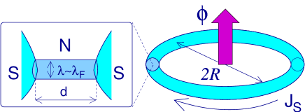
Figure 36: Superconducting ring with embedded SNS junction of length $d$ SZ .

VII.2.3 SNS rings

We now turn to the situations in which parity effect gains importance and can be directly probed in modern experiments. Let us slightly modify our system and consider a relatively thick superconducting ring with large $g_{\xi}\gg 1$ interrupted by a thin wire of length $d$ with only few conducting channels

$${\mathcal{N}}_{n}\sim 1$$ (196)

thus forming a weak link inside the superconducting ring, see Fig. 36. Without loss of generality this wire can be considered normal no matter if it is made of a normal or a superconducting material. In the latter case quantum fluctuations would fully suppress the order parameter inside such a wire bringing it into the normal state. In contrast, QPS effects in superconducting parts of the ring can be neglected thus making the mean field BCS description applicable. A clear advantage of these structures in comparison to homogeneous rings is that in the former case the effect of the electron parity number on PC can be large due to the condition (196).

In order to evaluate PC in such structures we again employ the parity projection formalism. According to eqs. (190), (191) we need to evaluate both the currents $I_{f/b}$ and the difference between the ”Fermi” and ”Bose” thermodynamic potentials $\Omega_{b}-\Omega_{f}\equiv\Omega_{bf}$. The currents $I_{f/b}$ can be conveniently expressed via the phase difference across the weak link $\varphi\simeq 2\pi\phi_{x}$ by means of the general formula GZ02

$$I_{f/b}=\frac{2e}{\hbar}\sum_{i=1}^{{\mathcal{N}}_{n}}T\sum_{\omega_{f/b}}\frac{\sin\varphi}{\cos\varphi+W_{i}(\omega_{f/b})},$$ (197)

where the sum runs over conducting channels of the normal wire and the function $W_{i}(\omega)$ was evaluated in Ref. GZ02 . The difference of thermodynamic potentials $\Omega_{bf}$ is defined as a sum of the contributions from superconducting ($\Omega_{bf}^{(s)}$) and normal ($\Omega_{bf}^{(n)}$) parts of the ring. The former is evaluated with the aid of eqs. (192), (193) which yield the standard result Tuo93

$$\beta\Omega_{bf}^{(r)}\simeq N_{0}{\mathcal{V}}\sqrt{\Delta_{0}T}e^{-\frac{\Delta_{0}}{T}},$$ (198)

while the latter is found by integrating $I_{f/b}(\varphi)$ (197) over the phase $\varphi$.

We now consider several important limiting cases. The first limit is that of a very short normal wire $d\rightarrow 0$. This is essentially the limit of a quantum point contact. In practice this limit is realized for $d\ll\xi$. Even smaller values of $d$ are required provided the contact transmission is small. In the limit of a quantum point contact one finds GZ02

$$W_{i}(\omega)=(2/{\mathcal{T}}_{i})(1+\hbar^{2}\omega^{2}/\Delta_{0}^{2})-1,$$ (199)

where ${\mathcal{T}}_{i}$ define transmissions of the conducting channels. Substituting this function into the above equations one arrives at the final result SZ ; SZ2

$$I_{e/o}=-\frac{2e}{\hbar}\sum_{i=1}^{N}\frac{\partial\varepsilon_{i}(\varphi)}{\partial\varphi}\tanh\frac{\varepsilon_{i}(\varphi)}{2T}$$

$$\times\left[1\pm\frac{(\coth\frac{\varepsilon_{i}(\varphi)}{2T})^{2}-1}{e^{\beta\Omega_{bf}^{(r)}}\prod\limits_{j=1}^{N}(\coth\frac{\varepsilon_{j}(\varphi)}{2T})^{2}\pm 1}\right].$$ (200)

Here $\varepsilon_{i}(\varphi)=\Delta\sqrt{1-{\mathcal{T}}_{i}\sin^{2}(\varphi/2)}$ are Andreev energy levels in a quantum point contact.

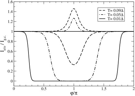
Figure 37: The ratio between canonical and grand canonical values of PC $I_{e/o}/I_{g.c.}$ (represented by the term in the square brackets in Eq. (200) versus $\varphi$ in a single mode QPC at different temperatures for even (three upper curves) and odd (three lower curves) ensembles. Here we have chosen the channel transmission ${\mathcal{T}}=0.99$ SZ .

The first line of eq. (200) defines the standard grand canonical result KO ; KO1 while the term in the square brackets accounts for the parity effect in our system. For ${\mathcal{N}}_{n}=1$ and at $T=0$ this term reduces to unity for even ensembles and to zero for odd ones, i.e. PC turns out to be totally blocked in the case of odd number of electrons SZ ; SZ2 ; FNJ .

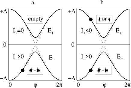
Figure 38: Andreev levels inside a quantum point contact and their occupation at $T=0$ for even (a) and odd (b) ensembles SZ .

The physics of this blocking effect is rather transparent and can be understood as follows. We first recall that in the limit $d\rightarrow 0$ the Josephson current can be expressed only via the contributions from discrete Andreev energy states $E_{\pm}=\pm\epsilon(\varphi)$ as Furusaki ; Furusaki1

$$I(\varphi)=\frac{2e}{\hbar}\left[\frac{\partial E_{-}}{\partial\varphi}f_{-}(E_{-})+\frac{\partial E_{+}}{\partial\varphi}f_{+}(E_{+})\right].$$ (201)

Using the Fermi filling factors for these states $f_{\pm}(E_{\pm})=[1+\exp(\pm\epsilon(\varphi)/T)]^{-1}$ one arrives at the standard grand canonical results KO ; KO1 . In the case of superconducting rings with fixed number of electrons $N$ these filling factors should be modified. Let us set $T\rightarrow 0$. For even $N$ all electrons are paired occupying available states with energies below the Fermi level (see Fig. 38a). In this case one has $f_{-}(E_{-})=1$, $f_{+}(E_{+})=0$, the current is entirely determined by the contribution of the quasiparticle state $E_{-}$ and eq. (201) yields the same result as one for the grand canonical ensemble. By contrast, in the case of odd $N$ one electron always remains unpaired and occupies the lowest available energy state – in our case $E_{+}$ – above the Fermi level. Hence, for odd $N$ one has $f_{\pm}(E_{\pm})=1$ (Fig. 38b), the contributions of the two Andreev states in eq. (201) exactly cancel each other, and the current remains zero for any $\varphi$ or the magnetic flux $\Phi_{x}$. This is just the effect of parity-induced blocking of PC derived above from formal considerations.

For $T>0$ Eq. (200) demonstrates that both for even and especially for odd $N$ the current-phase relation for QPC may substantially deviate from that derived for the grand canonical ensemble KO , see Fig. 37. For even ensembles the supercurrent increases above its grand canonical value. This effect is mainly pronounced for phases $\varphi$ not very far from $\varphi=\pi$ and – at sufficiently low $T$ – it becomes progressively more important with increasing temperature. On the contrary, for odd ensembles the supercurrent is always suppressed below its grand canonical value. This suppression is gradually lifted with increasing temperature, though at phases $\varphi$ in the vicinity of the point $\varphi=\pi$ blocking of PC may persist up to sufficiently high $T$. Eq. (200) also shows that in quantum point contacts with several conducting channels and at $T\rightarrow 0$ the current through the most transparent channel will be blocked by the odd electron. Hence, though blocking of PC remains incomplete in this case, it may nevertheless be important also for quantum point contacts with ${\mathcal{N}}_{n}>1$.

Let us now turn to another important limit of superconducting rings containing a normal wire of length $d>\xi_{0}\sim\hbar v_{F}/\Delta_{0}$. In contrast to the case $d\rightarrow 0$ considered above, the Josephson current in $SNS$ structures cannot anymore be attributed only to the discrete Andreev states inside a weak link, and an additional contribution from the states in the continuum should also be taken into account. Furthermore, for any non-zero $d$ there are always more than two discrete Andreev levels in the system. Accordingly, significant modifications in the physical picture of the parity effect in such SNS rings can be expected.

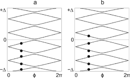
Figure 39: Andreev levels in a single mode $SNS$ junction with $d=6\hbar v_{F}/\Delta_{0}$ and their occupation at $T=0$ for even (a) and odd (b) ensembles SZ .

The key difference can be understood already by comparing the typical structure of discrete Andreev levels in SNS junctions (Fig. 39) with that of a quantum point contact (Fig. 38). As before, in the limit $T\rightarrow 0$ all states below (above) the Fermi level are occupied (empty) provided the total number of electrons in the system is even (Fig. 39a). If, on the other hand, this number is odd the lowest Andreev state above the Fermi energy is occupied as well (Fig. 39b) thus providing an additional contribution to the Josephson current. This contribution, however, cancels only that of a symmetric Andreev level below the Fermi energy, while the contributions of all other occupied Andreev levels and of the continuum states remain uncompensated. Hence, unlike in the case $d\rightarrow 0$, in $SNS$ rings one should not anymore expect the effect of PC blocking by the odd electron but rather some other non-trivial features of the parity effect.

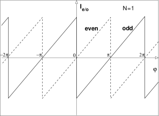
Figure 40: The zero temperature current-phase dependence (203) for SNS rings with ${\mathcal{N}}_{n}=1$: $I_{e}(\varphi)$ (dashed) line and $I_{o}(\varphi)$ (solid) line SZ .

This conclusion is fully confirmed by our quantitative analysis SZ ; SZ2 . Let us restrict our attention to transparent SNS junctions in which case the function $W_{i}(\omega)\equiv W(\omega)$ is the same for all transmission channels and reads GZ02

$$W(\omega)=\left(\frac{2\hbar^{2}\omega^{2}}{\Delta_{0}^{2}}+1\right)\cosh\left(\frac{2\omega d}{v_{F}}\right)$$

$$+\frac{2\hbar\omega}{\Delta_{0}}\sqrt{1+\frac{\hbar^{2}\omega^{2}}{\Delta_{0}^{2}}}\sinh\left(\frac{2\omega d}{v_{F}}\right).$$ (202)

Substituting this function into (197) and repeating the whole calculation as above, we arrive at the final result SZ ; SZ2 which takes a particularly simple form in the limit $T\rightarrow 0$ and $d\gg\xi_{0}$:

$$I_{e}=\frac{ev_{F}{\mathcal{N}}_{n}}{\pi d}\varphi,\;\;\;\;I_{o}=\frac{ev_{F}{\mathcal{N}}_{n}}{\pi d}\left(\varphi-\frac{\pi\mbox{sgn}\varphi}{{\mathcal{N}}_{n}}\right)$$ (203)

This result applies for $-\pi<\varphi<\pi$ and should be $2\pi$-periodically continued otherwise. We observe that at $T=0$ the current $I_{e}$ again coincides with that for the grand canonical ensembles Kulik ; Kulik1 , while in the case of odd ensembles the current-phase relation is shifted by the value $\pi/N$. This shift has a simple interpretation being related to the odd electron contribution $(2e/\hbar)\partial E_{1}/\partial\varphi$ from the lowest (above the Fermi level) Andreev state $E_{1}(\varphi)$ inside the SNS junction. As we have expected, this contribution indeed does not compensate for the current from other electron states. Rather it provides a possibility for a parity-induced $\pi$-junction state Leva in our system: According to Eq. (203) for single mode $SNS$ junctions the “sawtooth” current-phase relation will be shifted exactly by $\pi$, see Fig. 40. More generally, we can talk about a novel $\pi/N$-junction state, because in the odd case the minimum Josephson energy (zero current) state is reached at $\varphi=\pm\pi/N$, see Fig. 40. For any ${\mathcal{N}}_{n}>1$ this is a twofold degenerate state within the interval $-\pi<\varphi<\pi$. In the particular case ${\mathcal{N}}_{n}=2$ the current-phase relation $I_{o}(\varphi)$ turns $\pi$-periodic, see Fig. 41.

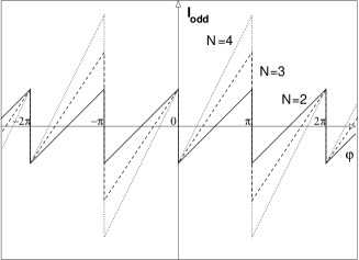
Figure 41: The same as in Fig. 40 only for the odd ensembles (second Eq. (203)) and for ${\mathcal{N}}_{n}=2,3$ and $4$ SZ .

Let us recall that the $\pi$-junction state can be realized in $SNS$ structures by driving the electron distribution function in the contact area out of equilibrium Volkov ; WSZ ; Yip . Here, in contrast, the situation of a $\pi$- or $\pi/N$-junction is achieved in thermodynamic equilibrium. Along with this important difference, there also exists a certain physical similarity between the effects discussed here and in Refs. Volkov ; WSZ ; Yip : In both cases the electron distribution function in the weak link deviates substantially from the Fermi function. It is this deviation which is responsible for the appearance of the $\pi$-junction state in both physical situations.

Perhaps the most spectacular physical consequence of the parity effect in SNS rings is the presence of spontaneous supercurrents in the ground state of such rings with odd number of electrons. Similarly to the case of standard $\pi$-junctions Leva such spontaneous supercurrents should flow even in the absence of an externally applied magnetic flux. Unlike in Ref. Leva , however, here the spontaneous current state occurs for any inductance of the ring because of the non-sinusoidal dependence $I_{o}(\varphi)$.

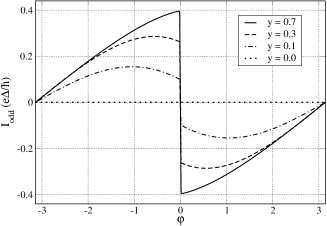
Figure 42: The zero temperature current-phase relation $I_{o}(\varphi)$ ($-\pi<\varphi<\pi$) for ${\mathcal{N}}_{n}=1$ and different values of the parameter $y=d\Delta/\hbar v_{F}$ SZ .

Consider, for instance, the limit $d\gg\hbar v_{F}/\Delta_{0}$. In the case of odd number of electrons the ground state energy of an SNS ring can be written in a simple form

$$E=\frac{\Phi^{2}}{2c{\mathcal{L}}}+\frac{\pi\hbar v_{F}{\mathcal{N}}_{n}}{\Phi_{0}^{2}d}\left(\Phi-\frac{\Phi_{0}\mbox{sgn}\Phi}{2{\mathcal{N}}_{n}}\right)^{2},$$ (204)

where the first term is the magnetic energy of the ring (${\mathcal{L}}$ is the ring inductance) while the second term represents the Josephson energy of an SNS junction. Minimizing (204) with respect to the flux $\Phi$ one immediately concludes that the ground state of the ring is a twofold degenerate state with a non-vanishing spontaneous current

$$I=\pm\frac{ev_{F}}{d}\left[1+\frac{2ev_{F}{\mathcal{N}}_{n}}{d}\frac{{\mathcal{L}}}{\Phi_{0}}\right]^{-1}$$ (205)

flowing either clockwise or counterclockwise. In the limit of small inductances ${\mathcal{L}}\rightarrow 0$ this current does not vanish and its amplitude just reduces to that of the odd electron current at $\varphi\rightarrow 0$. One finds SZ ; SZ2 :

$$I_{sp}=e\Delta_{0}^{2}d/\hbar^{2}v_{F},\;\;\;\; \;\;d\ll\hbar v_{F}/\Delta_{0},$$ (206)

$$I_{sp}=ev_{F}/\pi d,\;\;\;\; \;\;d\gg\hbar v_{F}/\Delta_{0}.$$ (207)

At $d\sim\hbar v_{F}/\Delta_{0}$ the amplitude of the current $I_{sp}$ can be evaluated numerically, see Fig. 43. One observes that – in agreement with eq. (206) – $I_{sp}$ increases linearly with $d$ at small $d$, reaches its maximum value $I_{\mathrm{max}}\sim 0.4e\Delta_{0}/\hbar$ at $d\sim\xi$ and then decreases with further increase of $d$ approaching the dependence (207) in the limit of large $d$. For generic BCS superconductors the magnitude of this maximum current can be estimated as $I_{\mathrm{max}}\sim 10\div 100$ nA. These values might be considered as surprisingly large ones having in mind that this current is associated with only one Andreev electron state.

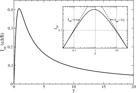
Figure 43: The spontaneous current amplitude $I_{sp}$ as a function of the parameter $y$ at $T=0$. In the inset, the same function is shown on the $log-log$ scale. Dashed lines indicate the asymptotic behavior of $I_{sp}(y)$ in the limits of small and large $y$ SZ .

Note that in the above analysis we merely assumed that the normal wire is sufficiently clean and, on top of that, is in a good electric contact with superconductors. Since both these assumptions can be violated in a realistic experiment it is important to discuss the corresponding modifications of our results.

Assume first that the transmissions of both NS interfaces are small $\mathcal{T}_{1,2}\ll 1$. In this limit electron transport across the junction is mainly due to resonant tunneling through discrete energy levels inside the normal metal. For simplicity we will restrict our analysis to a single channel junction ${\mathcal{N}}_{n}=1$. The most interesting physical situation is realized in the limit of short junction $d\ll\hbar v_{F}/\Delta_{0}$. In the case of a one dimensional metal of length $d$, the level spacing in the vicinity of the Fermi energy is $\delta\epsilon\sim\hbar v_{F}/d$. Hence, the condition for the short junction regime can also be represented in the form $\delta\epsilon\gg\Delta_{0}$. Electron tunneling causes a non-zero linewidth of the energy levels which is proportional to ${\mathcal{T}}_{1,2}\delta\epsilon$. This value is much smaller than $\delta\epsilon$, hence, the resonances remain well separated. In this situation it suffices to take into account only the closest level to the Fermi energy inside the normal metal.

As before, making use of eqs. (197) combined with the proper expression for the $W$-function GZ02 one finds SZ2

$$I_{f/b}=\frac{e}{\hbar}T\sum_{\omega_{f/b}}\frac{\Delta_{0}^{2}\mathcal{T}\sin\varphi}{\varepsilon^{2}(\varphi)+\omega_{f/b}^{2}\left(1+4\mathcal{D}\mathcal{T}/\mathcal{T}_{\mathrm{max}}\right)},$$ (208)

where

$$\mathcal{D}=\left(\frac{\Delta_{0}}{\Gamma}\right)^{2}\left(1+\frac{\omega_{f/b}^{2}}{\Delta_{0}^{2}}\right)+\frac{\Delta_{0}}{\Gamma}\sqrt{1+\frac{\omega_{f/b}^{2}}{\Delta_{0}^{2}}},$$ (209)

$\varepsilon(\varphi)=\Delta\sqrt{1-\mathcal{T}\sin^{2}(\varphi/2)}$, $\Gamma=\Gamma_{1}+\Gamma_{2}$, $\Gamma_{1,2}/\hbar=\mathcal{T}_{1,2}v_{F}/2d$ are the tunneling rates, $\mathcal{T}_{\mathrm{max}}=4\Gamma_{1}\Gamma_{2}/\Gamma^{2}$ and the total transmission probability at the Fermi energy $\mathcal{T}$ is given by the Breit-Wigner formula

$$\mathcal{T}=\frac{\Gamma_{1}\Gamma_{2}}{\left(\epsilon_{R}\right)^{2}+\frac{1}{4}\Gamma^{2}},$$

where $\epsilon_{R}$ is the energy of a resonant level.

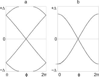
Figure 44: Andreev levels in a single mode $SNS$ junction with $d=\hbar v_{F}/\Delta$: (a) $\mathcal{T}_{1,2}=1$ and (b) $\mathcal{T}_{1,2}\ll 1$ and $\Delta/\Gamma=0.5$. In both cases $\mathcal{T}=1$ SZ2 .

It follows from Eqs. (208), (209) that – although the transparencies of both barriers are low – the total transmission $\mathcal{T}$ and, hence, the Josephson current shows sharp peaks provided the Fermi energy becomes close to a bound state inside the junction. On the other hand, eqs. (208), (209) demonstrate that even in the vicinity of resonances the behavior of the Josephson current as a function of the phase difference $\varphi$ and temperature $T$ can substantially deviate from that for transparent $SNS$ junctions.

In order to understand the physical reasons for such a difference it is instructive to compare the structure of discrete Andreev levels for ballistic ($\mathcal{T}_{1,2}=1$) SNS junctions with that for junctions with weakly transmitting NS interfaces $\mathcal{T}_{1,2}\ll 1$, see Fig. 44. The spectrum of the latter system consists only of a single non-degenerate state $\varepsilon_{0}(\varphi)$ in the interval $0<\varepsilon_{0}<\Delta_{0}$ (Fig. 44b). As a result, the behavior of $\varepsilon_{0}(\varphi)$ at small $\varphi$ is smooth and the derivative of $\varepsilon_{0}$ with respect to $\varphi$ has no jump at $\varphi=0$. In contrast, in the case of ballistic SNS junctions discrete levels become split at arbitrary small values of the phase $\varphi$ (Fig. 44a) and the derivative of the lowest Andreev level with respect to $\varphi$ acquires a jump at $\varphi=0$. As this feature is absent in resonant SNS junctions the spontaneous current in the ground state of such systems can only develop at not very small ring inductances. The results for PC in SNS rings with resonant transmission are presented in Fig. 45. They clearly demonstrate that at sufficiently low temperatures the “$\pi$-junction” state should be realized in the case of odd number of electrons.

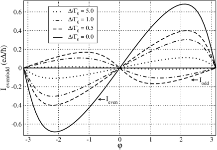
Figure 45: Zero temperature current-phase relations $I_{e/o}(\varphi)$ for $\mathcal{T}=0.9$, $\Gamma_{1}=\Gamma_{2}=\Gamma_{0}$ and different values of the parameter $\Delta_{0}/\Gamma_{0}$ SZ2 .

Finally let us turn to the case of a disordered normal wire. The difference between PC values for odd ($I_{o}$) and even ($I_{e}$) ensembles is related to the minigap value $\varepsilon_{g}(\varphi)$ inside the normal metal GK ; BBS2 ; Been ; Pilgram ; Zhou ; KKZ . This relation acquires a particularly simple form in the limit $T\rightarrow 0$:

$$I_{o}(\Phi)=I_{e}(\Phi)+2e\frac{\partial\varepsilon_{g}(\varphi)}{\partial\varphi}.$$ (210)

The last term in this equation describes the contribution to the current from the “odd” electron occupying the lowest available state above the minigap $\varepsilon_{g}(\varphi)$ in the density of states of the normal metal.

Let us first evaluate PC for the even ensemble $I_{e}$. As before, at $T=0$ this current identically coincides with one calculated for the grand canonical ensemble. The results for the current-phase relation $I_{e}(\varphi)$ are displayed in Fig. 46 at various impurity concentrations. PC in the odd ensemble $I_{o}$ at $T=0$ can be evaluated from eq. (210). Combining our results for $I_{e}(\varphi)$ with those for the minigap $\varepsilon_{g}(\varphi)$ derived in Ref. KKZ we arrive at a typical dependence $I_{o}(\varphi)$ displayed in Fig. 46. We observe that at sufficiently large values of $\varphi<\pi$ the absolute value of the odd electron contribution to PC $2e\partial\varepsilon_{g}/\partial\varphi$ exceeds the term $I_{e}(\varphi)$ and the total current $I_{o}$ changes the sign. This non-trivial parity-affected current-phase relation is specific for SNS rings with disorder and it substantially differs from the current-phase relations derived above for SNS rings with ballistic and resonant transmissions.

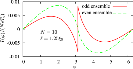
Figure 46: Phase dependence of the Josephson current at $T=0$ for the odd and even number of electrons in the ring KKZ .

At the same time, as in the previous cases, in the odd ensemble there exists a possibility both for a $\pi$-junction state and for spontaneous currents in the ground state of the system without any externally applied magnetic flux. Let us evaluate the ground state energy of the SNS junction by integrating Eq. (210) with respect to the phase $\varphi$. One finds

$$E_{o}(\varphi)=E_{e}(\varphi)-\varepsilon_{g}(0)+\varepsilon_{g}(\varphi),\;\;\;E_{e}(\varphi)=\frac{1}{2e}\int\limits_{0}^{\varphi}I_{e}(\varphi)d\varphi,$$ (211)

where $E_{e/o}(\varphi)$ are the ground state energies of SNS junction for even and odd number of electrons in the ring. While the energy $E_{e}(\varphi)$ is always non-negative and reaches its minimum at $\varphi=0$, in the odd case the ground state energy $E_{o}(\varphi)$ can become negative reaching its absolute minimum at $\varphi=\pi$. This physical situation of a $\pi$-junction is illustrated in Fig. 47.

It is easy to find out under which conditions the $\pi$-junction state becomes possible. For that purpose it is sufficient to observe that for any impurity concentration $E_{e}(\pi)=\alpha I_{C}/e$, where $I_{C}$ is the grand canonical critical current at $T=0$ and the prefactor $\alpha\sim 1$ depends on the form of the current-phase relation. The $\pi$-junction condition $E_{o}(\pi)<0$ is equivalent to the inequality

$$\varepsilon_{g}(0)>\alpha I_{C}/e.$$ (212)

It is obvious from Fig. 47 that in the many channel limit the inequality (212) cannot be satisfied for sufficiently large $l$. On the other hand, for sufficiently short mean free paths $I_{C}\propto l^{2}$ decays faster with decreasing $l$ as compared to the minigap $\varepsilon_{g}(0)\propto l$, and the $\pi$-junction state becomes possible. In particular, in the diffusive limit one finds Dubos $I_{C}\simeq 10.82\varepsilon_{\mathrm{Th}}/eR_{N}=1.53e{\mathcal{N}}_{n}v_{F}l^{2}/d^{3}$ and $\alpha\simeq 1.05$, where $R_{N}$ is the Drude resistance of a normal metal.

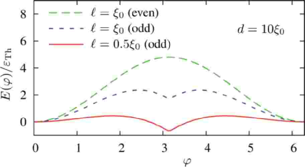
Figure 47: Josephson energy $E(\varphi)$ of an SNS ring as a function of the phase difference $\varphi$ for the even and odd ensembles. The solid curve corresponds to a $\pi$-junction state KKZ .

Combining these results with the expression for the minigap BBS2 ; Zhou $\varepsilon_{g}(0)\simeq 3.12\varepsilon_{\mathrm{Th}}$, from the condition (212) we observe that in the odd case the $\pi$-junction state is realized provided the number of conducting channels in the junction ${\mathcal{N}}_{n}$ is smaller than

$${\mathcal{N}}_{n}<0.65d/l.$$ (213)

This condition is not very restrictive and it can certainly be achieved in various experiments. For sufficiently dirty junctions it allows for a formation of the $\pi$-junction state even in the many channel limit. The condition (213) can also be rewritten as $g_{N}<1.73$, where $g_{N}=8{\mathcal{N}}_{n}l/3d$ is dimensionless conductance of a normal wire.

The condition for the presence of spontaneous currents in the ground state of SNS rings with an odd number of electrons is established analogously, one should only take into account an additional energy of the magnetic field produced by PC circulating inside the ring. The ground state with spontaneous currents is possible provided the total energy of the ring $E_{\mathrm{tot}}(\pi)$ becomes negative, i.e.

$$E_{\mathrm{tot}}(\pi)=1.8\varepsilon_{\mathrm{Th}}\left[g_{N}-1.73\right]+\frac{(\Phi_{0}/2)^{2}}{2\mathcal{L}}<0.$$ (214)

This condition is more stringent than that for the $\pi$-junction state, but can also be satisfied provided ${\mathcal{L}}$ exceeds a certain threshold value which can roughly be estimated as $\sim 0.1\Phi_{0}^{2}/\varepsilon_{\mathrm{Th}}$.

We conclude that in the diffusive limit the current-phase relation in the odd case is entirely different from that in the ballistic case. Also the restriction on the number of conducting channels ${\mathcal{N}}_{n}$ in the normal metal (213) is less stringent. This feature of diffusive SNS rings is rather advantageous for possible experimental observation of the effects discussed here.

Still, in practice it would be necessary to fabricate SNS rings with few conducting channels in the normal wire ${\mathcal{N}}_{n}\lesssim 10$. This condition can hardly be met for conventional normal metals. It appears, therefore, that most promising candidates for practical realization of such structures are junctions with N-layers formed by carbon nanotubes or organic molecules. In this respect it is important to point out that observations of clear signatures of dc Josephson effect in superconducting junctions with a weak link formed by carbon nanotubes were reported by several experimental groups Kas ; Delft ; VBou ; L1 ; L2 ; Hels Also intrinsic superconductivity in carbon was claimed HBou ; HBou2 ; Jap , though at this stage it appears that more experimental support for these claims would be desirable. Regardless of this latter issue, SNS junctions with carbon nanotubes are most likely objects in which it would be possible to observe the influence of the parity effect on persistent currents in superconducting nanorings.

VIII Summary

It is well established that fluctuations play an important role in structures with reduced dimensionality. In superconducting materials clear signatures of fluctuation effects exist already above the critical temperature $T_{C}$ almt ; Maki ; Thomson ; LV . Also $T_{C}$ itself can be reduced due to fluctuation effects. This reduction is particularly important in disordered 2D films and quasi-1D wires Fin . In this paper we addressed fluctuation effects which occur in ultra-thin superconducting wires at temperatures below the mean field BCS critical temperature. Superconducting properties of such systems have been intensively studied – both theoretically and experimentally – during past years. The key conclusions of these investigations can be summarized as follows.

Thicker superconducting wires are characterized by very small Ginzburg numbers $Gi_{1D}\lll$1 and diameters typically $\gtrsim$ 100 nm. In such systems the superconducting transition is broadened due to thermally activated phase slips (TAPS) la ; mh which cause non-zero resistance $R(T)$ at temperatures close enough to the critical temperature $T_{C}-T\ll T_{C}$. Upon decreasing temperature TAPS events become less likely and quantum fluctuations of the order parameter take over. This is the regime of quantum phase slips (QPS) which sets in at $T\lesssim\Delta_{0}(T)$. As long as the wire is sufficiently thick and the Ginzburg number remains very small, $Gi_{1D}\lll$1, QPS events are rare and typically do not lead to any measurable consequences. Hence, the behavior of thicker wires remains essentially superconducting outside an immediate vicinity of the critical temperature. Upon reduction of the wire diameter below $\sim$50 nm the QPS rate increases drastically. In this regime the wire resistance $R(T)$ still decreases with temperature but may remain well in the measurable range down to very low $T$. Provided the wire diameter is decreased further the dimensionless conductance of a wire segment of length $\xi$ eventually becomes of order $g_{\xi}\sim$10 or smaller. In such wires QPS proliferate causing a sharp crossover from a superconducting to a normal behavior. For generic parameters this crossover is expected for wire diameters in the 10 nm range ZGOZ ; ZGOZ2 ; GZ01 . This crossover was indeed observed in a number of experiments in wires with thicknesses exactly in this range. Thus, intrinsic superconductivity in wires with diameters $\lesssim$ 10 nm is destroyed by quantum fluctuations of the order parameter at any temperature down to $T=0$.

Theoretical analysis of nanowires reveals further interesting effects, like QPS-binding-unbinding quantum phase transition (QPT) ZGOZ between superconducting and non-superconducting phases which is predicted to occur as the impedance of a superconducting wire becomes of order of the quantum resistance unit $R_{q}\approx$ 6.5 k$\Omega$. For typical parameters this condition is also achieved for wire diameters in the 10 nm range. To the best of our knowledge, no clear experimental evidence for this phase transition exists so far. This can be due to rather stringent requirements: QPT can only be observed in long nanowires at sufficiently low temperatures, ideally at $T\to 0$. Interesting effects may occur also in short nanowires forming weak links between superconducting electrodes. In many respects such systems can behave similarly to Josephson nanojunctions and weak links.

Novel effects are also expected in superconducting nanorings. While rings formed by thicker wires demonstrate the standard behavior familiar from the bulk samples, the situation changes drastically as soon as the wire thickness gets reduced down to $\approx$ 10 nm or below this value. In this case QPS effects become important leading to strong fluctuations of the magnetic flux inside the ring. As a result, the amplitude of persistent current decreases and its flux dependence changes from the sawtooth-like to a smoother one MLG . For such rings even at $T=0$ persistent current gets exponentially suppressed by quantum fluctuations provided the ring radius $R$ exceeds the critical scale $R_{c}\sim\xi\exp(S_{\rm core}/2)$ where $S_{\rm core}\sim g_{\xi}\sim Gi_{1D}^{-3/2}$ is the action of the QPS core. For typical wire parameters the length $R_{c}$ can be of order of a micron or even smaller. This length constitutes another fundamental scale associated with quantum phase slips.

Yet another important factor which may influence persistent currents in isolated superconducting nanorings is the electron parity number. This influence is particularly strong in nanorings containing a weak link with few conducting modes. Changing the electron parity number from even to odd may result in spontaneous supercurrent in the ground state of such rings without any externally applied magnetic flux SZ . At $T=0$ this current is produced by the only unpaired electron which occupies the lowest available Andreev state. Under certain conditions this spontaneous supercurrent can reach remarkably large values up to $\sim e\Delta_{0}/\hbar\sim 10\div 100$ nA which can be reliably detected in modern experiments.

IX Acknowledgements

We gratefully acknowledge collaboration and/or helpful discussions with A.A. Bezryadin, G. Blatter, A.V. Galaktionov, M.S. Kalenkov, C.N. Lau, J.E. Mooij, Yu.V. Nazarov, Y. Oreg, A. van Otterlo, L. Pryadko, G. Schön, S.V. Sharov, M. Tinkham, D. Vodolazov and G.T. Zimanyi. This work was supported in part by the European Community’s Framework Programme NMP4-CT-2003-505457 ULTRA-1D ”Experimental and theoretical investigation of electron transport in ultra-narrow 1-dimensional nanostructures” and by RFBR Grant 06-02-17459.

Appendix A Equilibrium Green-Keldysh functions

We formally define the sub-blocks $\hat{G},\hat{F},\hat{\bar{G}},\hat{\bar{F}}$ in the Green-Keldysh matrix (26) by means of the following equations:

$$\hat{G}=\frac{1}{i}\left(\begin{array}[c]{cc}\langle{\mathcal{T}}\hat{\psi}_{\uparrow}(X_{1})\hat{\psi}^{\dagger}_{\uparrow}(X_{2})\rangle&-\langle\hat{\psi}^{\dagger}_{\uparrow}(X_{2})\hat{\psi}_{\uparrow}(X_{1})\rangle\\ \langle\hat{\psi}_{\uparrow}(X_{1})\hat{\psi}_{\uparrow}^{\dagger}(X_{2})\rangle&\langle{\mathcal{T}}^{-1}\hat{\psi}_{\uparrow}(X_{1})\hat{\psi}_{\uparrow}^{\dagger}(X_{2})\rangle\end{array}\right),$$ (217)

$$\hat{F}=\frac{1}{i}\left(\begin{array}[c]{cc}\langle{\mathcal{T}}\hat{\psi}_{\uparrow}(X_{1})\hat{\psi}_{\downarrow}(X_{2})\rangle&-\langle\hat{\psi}_{\downarrow}(X_{2})\hat{\psi}_{\uparrow}(X_{1})\rangle\\ \langle\hat{\psi}_{\uparrow}(X_{1})\hat{\psi}_{\downarrow}(X_{2})\rangle&\langle{\mathcal{T}}^{-1}\hat{\psi}_{\uparrow}(X_{1})\hat{\psi}_{\downarrow}(X_{2})\rangle\end{array}\right),$$ (220)

$$\hat{\bar{F}}=\frac{1}{i}\left(\begin{array}[c]{cc}\langle{\mathcal{T}}\hat{\psi}_{\downarrow}^{\dagger}(X_{1})\hat{\psi}_{\uparrow}^{\dagger}(X_{2})\rangle&-\langle\hat{\psi}_{\uparrow}^{\dagger}(X_{2})\hat{\psi}_{\downarrow}^{\dagger}(X_{1})\rangle\\ \langle\hat{\psi}_{\downarrow}^{\dagger}(X_{1})\hat{\psi}_{\uparrow}^{\dagger}(X_{2})\rangle&\langle{\mathcal{T}}^{-1}\hat{\psi}_{\downarrow}^{\dagger}(X_{1})\hat{\psi}_{\uparrow}^{\dagger}(X_{2})\rangle\end{array}\right),$$ (223)

$$\hat{\bar{G}}=\frac{1}{i}\left(\begin{array}[c]{cc}\langle{\mathcal{T}}\hat{\psi}^{\dagger}_{\downarrow}(X_{1})\hat{\psi}_{\downarrow}(X_{2})\rangle&-\langle\hat{\psi}_{\downarrow}(X_{2})\hat{\psi}^{\dagger}_{\downarrow}(X_{1})\rangle\\ \langle\hat{\psi}^{\dagger}_{\downarrow}(X_{1})\hat{\psi}_{\downarrow}(X_{2})\rangle&\langle{\mathcal{T}}^{-1}\hat{\psi}^{\dagger}_{\downarrow}(X_{1})\hat{\psi}_{\downarrow}(X_{2})\rangle\end{array}\right).$$ (226)

Here $\hat{\psi}_{\alpha},\hat{\psi}_{\alpha}^{\dagger}$ are the electron annihilation and creation operators, the symbol ${\mathcal{T}}$ (${\mathcal{T}}^{-1}$) stands for the time (anti-time) ordering.

Let us introduce the complete basis of the eigenfunctions $\chi_{n}(\bm{r})$ of the single electron Hamiltonian $H_{0}$:

$$H_{0}\chi_{n}(\bm{r})=\xi_{n}\chi_{n}(\bm{r}).$$ (227)

Here $\xi_{n}$ are the electron eneries in the normal state. Defining the quasiparticle energies in the superconducting state $E_{n}=\sqrt{\xi_{n}^{2}+\Delta_{0}^{2}}$ as well as the BCS coherence factors

$$u_{n}^{2}=\frac{1}{2}\left(1+\frac{\xi_{n}}{E_{n}}\right),\;\;v_{n}^{2}=\frac{1}{2}\left(1-\frac{\xi_{n}}{E_{n}}\right),$$ (228)

we arrive at the explicit expressions for the sub-blocks $\hat{G},\hat{F},\hat{\bar{G}},\hat{\bar{F}}$:

$$i\hat{G}(t,\bm{r}_{1},\bm{r}_{2}) =\sum_{n}\chi_{n}(\bm{r}_{1})\chi_{n}(\bm{r}_{2})\left[u_{n}^{2}\hat{A}_{n}(t)+v_{n}^{2}\hat{B}_{n}(t)\right],$$

$$i\hat{\bar{G}}(t,\bm{r}_{1},\bm{r}_{2}) =\sum_{n}\chi_{n}(\bm{r}_{1})\chi_{n}(\bm{r}_{2})\left[v_{n}^{2}\hat{A}_{n}(t)+u_{n}^{2}\hat{B}_{n}(t)\right],$$

$$i\hat{F}(t,\bm{r}_{1},\bm{r}_{2}) =i\hat{\bar{F}}(t,\bm{r}_{1},\bm{r}_{2})=\sum_{n}\chi_{n}(\bm{r}_{1})\chi_{n}(\bm{r}_{2})u_{n}v_{n}$$

$$\times\,\left[\hat{A}_{n}(t)-\hat{B}_{n}(t)\right],$$ (229)

where

$$\hat{A}_{n}(t) =e^{-iE_{n}t}\left(\begin{array}[c]{cc}\theta(t)-f_{n}&-f_{n}\\ 1-f_{n}&\theta(-t)-f_{n}\end{array}\right),$$ (232)

$$\hat{B}_{n}(t) =e^{iE_{n}t}\left(\begin{array}[c]{cc}f_{n}-\theta(-t)&-(1-f_{n})\\ f_{n}&f_{n}-\theta(t)\end{array}\right).$$ (235)

Here we introduced the occupation probabilities of the quasiparticle states $f_{n}$. In thermodynamic equilibrium these filling factors take the universal form

$$f_{n}=\frac{1}{1+e^{E_{n}/T}}.$$ (236)

Appendix B Ward identities

One can demonstrate that the matrix Green-Keldysh functions satisfy the following Ward identities

$$i\hat{F}\hat{\beta}+i\hat{\beta}\hat{F} =\hat{G}\hat{\sigma}_{z}\left(-\hat{\dot{\beta}}+\frac{i}{2m}\{\nabla,\hat{\beta}\}\right)\hat{F}$$

$$+\,\hat{F}\hat{\sigma}_{z}\left(\hat{\dot{\beta}}+\frac{i}{2m}\{\nabla,\hat{\beta}\}\right)\hat{\bar{G}}$$

$$+\,2i\Delta_{0}\hat{G}\hat{\sigma}_{z}\hat{\beta}\hat{\bar{G}}-2i\Delta_{0}\hat{F}\hat{\sigma}_{z}\hat{\beta}\hat{F},$$

$$-i\hat{\bar{F}}\hat{\beta}-i\hat{\beta}\hat{\bar{F}} =\hat{\bar{F}}\hat{\sigma}_{z}\left(-\hat{\dot{\beta}}+\frac{i}{2m}\{\nabla,\hat{\beta}\}\right)\hat{G}$$

$$+\,\hat{\bar{G}}\hat{\sigma}_{z}\left(\hat{\dot{\beta}}+\frac{i}{2m}\{\nabla,\hat{\beta}\}\right)\hat{\bar{F}}$$

$$+\,2i\Delta_{0}\hat{\bar{F}}\hat{\sigma}_{z}\hat{\beta}\hat{\bar{F}}-2i\Delta_{0}\hat{\bar{G}}\hat{\sigma}_{z}\hat{\beta}\hat{G},$$ (237)

$$\hat{G}\hat{\beta}-\hat{\beta}\hat{G} =i\hat{G}\hat{\sigma}_{z}\left(-\hat{\dot{\beta}}+\frac{i}{2m}\{\nabla,\hat{\beta}\}\right)\hat{G}$$

$$-\,i\hat{F}\hat{\sigma}_{z}\left(\hat{\dot{\beta}}+\frac{i}{2m}\{\nabla,\hat{\beta}\}\right)\hat{\bar{F}},$$

$$\hat{\bar{G}}\hat{\beta}-\hat{\beta}\hat{\bar{G}} =i\hat{\bar{F}}\hat{\sigma}_{z}\left(-\hat{\dot{\beta}}+\frac{i}{2m}\{\nabla,\hat{\beta}\}\right)\hat{F}$$

$$-\,i\hat{\bar{F}}\hat{\sigma}_{z}\left(\hat{\dot{\beta}}+\frac{i}{2m}\{\nabla,\hat{\beta}\}\right)\hat{\bar{F}},$$ (238)

where

$$\hat{\beta}=\left(\begin{array}[c]{cc}\beta_{F}(t,{\bm{r}})&0\\ 0&\beta_{B}(t,{\bm{r}})\end{array}\right)$$ (241)

is an arbitrary diagonal $2\times 2$ matrix.

Appendix C Kernels

Explicit expressions for the functions $\chi_{J}$ read

$$\chi_{\Delta}(Q) =-\frac{2N_{0}}{\lambda}+\frac{N_{0}}{\pi}\int d\xi_{1}d\xi_{2}\frac{Dq^{2}}{(\xi_{1}-\xi_{2})^{2}+D^{2}q^{4}}$$

$$\times\,\bigg{\{}-\left(1+\frac{\xi_{1}\xi_{2}-\Delta_{0}^{2}}{E_{1}E_{2}}\right)\frac{(E_{1}+E_{2})(1-f_{1}-f_{2})}{(\omega+i0)^{2}-(E_{1}+E_{2})^{2}}$$

$$+\,\left(1-\frac{\xi_{1}\xi_{2}-\Delta_{0}^{2}}{E_{1}E_{2}}\right)\frac{(E_{1}-E_{2})(f_{1}-f_{2})}{(\omega+i0)^{2}-(E_{1}-E_{2})^{2}}\bigg{\}},$$ (242)

$$\chi_{J}(Q) =-\frac{2e^{2}N_{0}}{\pi}\int d\xi_{1}d\xi_{2}\frac{Dq^{2}}{(\xi_{1}-\xi_{2})^{2}+D^{2}q^{4}}\frac{\Delta_{0}^{2}}{E_{1}E_{2}}$$

$$\times\,\bigg{\{}\frac{(E_{1}+E_{2})(1-f_{1}-f_{2})}{(\omega+i0)^{2}-(E_{1}+E_{2})^{2}}$$

$$+\,\frac{(E_{1}-E_{2})(f_{1}-f_{2})}{(\omega+i0)^{2}-(E_{1}-E_{2})^{2}}\bigg{\}},$$ (243)

$$\chi_{L}(Q) =-\frac{2m^{2}N_{0}D}{\pi}\int d\xi_{1}d\xi_{2}\frac{(\xi_{1}-\xi_{2})^{2}}{(\xi_{1}-\xi_{2})^{2}+D^{2}q^{4}}\frac{\Delta_{0}^{2}}{E_{1}E_{2}}$$

$$\times\,\bigg{\{}\frac{(E_{1}+E_{2})(1-f_{1}-f_{2})}{(\omega+i0)^{2}-(E_{1}+E_{2})^{2}}$$

$$+\,\frac{(E_{1}-E_{2})(f_{1}-f_{2})}{(\omega+i0)^{2}-(E_{1}-E_{2})^{2}}\bigg{\}},$$ (244)

$$\chi_{D}(Q) =\frac{e^{2}N_{0}D}{\pi}\int d\xi_{1}d\xi_{2}\frac{1}{(\xi_{1}-\xi_{2})^{2}+D^{2}q^{4}}$$

$$\times\,\bigg{\{}\left(1+\frac{\xi_{1}\xi_{2}+\Delta_{0}^{2}}{E_{1}E_{2}}\right)\frac{(E_{1}-E_{2})(f_{1}-f_{2})}{(\omega+i0)^{2}-(E_{1}-E_{2})^{2}}$$

$$-\,\left(1-\frac{\xi_{1}\xi_{2}+\Delta_{0}^{2}}{E_{1}E_{2}}\right)\frac{(E_{1}+E_{2})(1-f_{1}-f_{2})}{(\omega+i0)^{2}-(E_{1}+E_{2})^{2}}\bigg{\}}.$$ (245)

Here we defined $E_{1,2}=\sqrt{\xi_{1,2}^{2}+\Delta_{0}^{2}}$, $f_{1,2}=1/(1+\exp[E_{1,2}/T])$.

In a number of limiting cases the kernels $\chi_{j}$ can be evaluated exactly. First let us set $T=0$ and consider the limit of small wave vectors $Dq^{2}\ll|\omega|,\Delta_{0}$. This regime is relevant, e.g., in the context of microwave absorption. At $|\omega|<2\Delta_{0}$ we find

$$\chi_{\Delta} =-2N_{0}\frac{\sqrt{4\Delta_{0}^{2}-\omega^{2}}}{\omega}\arctan\frac{\omega}{\sqrt{4\Delta_{0}^{2}-\omega^{2}}},$$

$$\chi_{J} =\frac{8e^{2}N_{0}\Delta_{0}^{2}}{\omega\sqrt{4\Delta_{0}^{2}-\omega^{2}}}\arctan\frac{\omega}{\sqrt{4\Delta_{0}^{2}-\omega^{2}}},$$

$$\chi_{L} =\frac{2m^{2}\sigma_{D}\Delta_{0}}{e^{2}}K\left(\frac{\omega}{2\Delta_{0}}\right),$$

$$\chi_{D} =\frac{2\sigma_{D}\Delta_{0}}{\omega^{2}}\left[K\left(\frac{\omega}{2\Delta_{0}}\right)-E\left(\frac{\omega}{2\Delta_{0}}\right)\right],$$ (246)

while at $|\omega|>2\Delta_{0}$ one finds

$$\chi_{\Delta} =-2N_{0}\frac{\sqrt{\omega^{2}-4\Delta_{0}^{2}}}{\omega}\left[\ln\left(\frac{\omega}{2\Delta_{0}}+\sqrt{\frac{\omega^{2}}{4\Delta_{0}^{2}}-1}\right)-i\frac{\pi}{2}\right],$$

$$\chi_{J} =-\frac{8e^{2}N_{0}\Delta_{0}^{2}}{\omega\sqrt{\omega^{2}-4\Delta_{0}^{2}}}\left[\ln\left(\frac{\omega}{2\Delta_{0}}+\sqrt{\frac{\omega^{2}}{4\Delta_{0}^{2}}-1}\right)-i\frac{\pi}{2}\right],$$

$$\chi_{L} =\frac{2m^{2}\sigma_{D}\Delta_{0}}{e^{2}}\left[\frac{2\Delta_{0}}{\omega}K\left(\frac{2\Delta_{0}}{\omega}\right)\right.$$

$$\left.+\,i\frac{4\Delta_{0}}{\omega+2\Delta_{0}}K\left(\frac{\omega-2\Delta_{0}}{\omega+2\Delta_{0}}\right)\right],$$

$$\chi_{D} =\frac{\sigma_{D}}{\omega}\left[K\left(\frac{2\Delta_{0}}{\omega}\right)-E\left(\frac{2\Delta_{0}}{\omega}\right)\right]$$

$$+\,i\frac{\sigma_{D}}{\omega}\left[\left(1+\frac{2\Delta_{0}}{\omega}\right)E\left(\frac{\omega-2\Delta_{0}}{\omega+2\Delta_{0}}\right)\right.$$

$$\left.-\,\frac{4\Delta_{0}}{\omega+2\Delta_{0}}K\left(\frac{\omega-2\Delta_{0}}{\omega+2\Delta_{0}}\right)\right].$$ (247)

Here and below $K(x)$ and $E(x)$ are complete elliptic integrals of the first and second kind respectively. Utilizing the relation (56) one can verify that the expressions for $\chi_{L}$ and $\chi_{D}$ agree with the well known results MB , AG .

At temperatures close to $T_{C}$ one can derive analytic expressions for the kernels in the limit $|\omega|,Dq^{2},\Delta_{0}\ll 2\pi T_{C}$. At $|\omega|<2\Delta_{0}$ these expressions read

$$\chi_{\Delta} =-\frac{7\zeta(3)}{2\pi^{2}}\frac{N_{0}\Delta_{0}^{2}}{T^{2}}-\frac{N_{0}}{2T}\frac{|\omega|Dq^{2}}{2\Delta_{0}}\left[\frac{\pi\Delta_{0}}{|\omega|}+K\left(\frac{\omega}{2\Delta_{0}}\right)\right.$$

$$\left.-\frac{\omega^{2}+D^{2}q^{4}-4\Delta_{0}^{2}}{\omega^{2}+D^{2}q^{4}}\Pi\left(\frac{\omega^{2}}{\omega^{2}+D^{2}q^{4}},\frac{\omega}{2\Delta_{0}}\right)\right]$$

$$+\,i\frac{N_{0}\Delta_{0}}{T}\frac{\omega}{Dq^{2}}\left[\left(1-\frac{\omega^{2}}{4\Delta_{0}^{2}}\right)K\left(\sqrt{1-\frac{\omega^{2}}{4\Delta_{0}^{2}}}\right)\right.$$

$$\left.+\,\left(\frac{\omega^{2}}{4\Delta_{0}^{2}}-1+\frac{D^{2}q^{4}}{\omega^{2}+D^{2}q^{4}}\right)\right.$$

$$\times\,\left.\Pi\left(\frac{D^{2}q^{4}}{\omega^{2}+D^{2}q^{4}},\sqrt{1-\frac{\omega^{2}}{4\Delta_{0}^{2}}}\right)\right],$$ (248)

$$\chi_{J} =\frac{7\zeta(3)}{2\pi^{2}}\frac{e^{2}N_{0}\Delta_{0}^{2}}{T^{2}}$$

$$+\,\frac{e^{2}N_{0}\Delta_{0}}{T}\frac{|\omega|Dq^{2}}{\omega^{2}+D^{2}q^{4}}\Pi\left(\frac{\omega^{2}}{\omega^{2}+D^{2}q^{4}},\frac{\omega}{2\Delta_{0}}\right)$$

$$-\,i\frac{e^{2}N_{0}\Delta_{0}}{T}\frac{\omega}{Dq^{2}}\left[K\left(\sqrt{1-\frac{\omega^{2}}{4\Delta_{0}^{2}}}\right)-\frac{\omega^{2}}{\omega^{2}+D^{2}q^{4}}\right.$$

$$\times\,\left.\Pi\left(\frac{D^{2}q^{4}}{\omega^{2}+D^{2}q^{4}},\sqrt{1-\frac{\omega^{2}}{4\Delta_{0}^{2}}}\right)\right],$$ (249)

$$\chi_{L} =\frac{2m^{2}N_{0}D\Delta_{0}^{2}}{T}\left[\frac{\pi}{2}+\frac{|\omega|}{2\Delta_{0}}K\left(\frac{|\omega|}{2\Delta_{0}}\right)\right.$$

$$\left.-\,\frac{|\omega|}{2\Delta_{0}}\frac{D^{2}q^{4}}{\omega^{2}+D^{2}q^{4}}\Pi\left(\frac{\omega^{2}}{\omega^{2}+D^{2}q^{4}},\frac{\omega}{2\Delta_{0}}\right)\right]$$

$$-\,i\frac{m^{2}N_{0}D\Delta_{0}}{T}\frac{\omega^{3}}{\omega^{2}+D^{2}q^{4}}\Pi\left(\frac{D^{2}q^{4}}{\omega^{2}+D^{2}q^{4}},\sqrt{1-\frac{\omega^{2}}{4\Delta_{0}^{2}}}\right).$$ (250)

Here $\Pi(x,y)$ is the complete elliptic integral of the third kind. At higher frequencies $|\omega|>2\Delta_{0}$ we find

$$\chi_{\Delta} =-\frac{7\zeta(3)}{2\pi^{2}}\frac{N_{0}\Delta_{0}^{2}}{T^{2}}-\frac{N_{0}}{2T}Dq^{2}\left[\frac{\pi}{2}+K\left(\frac{2\Delta_{0}}{\omega}\right)\right.$$

$$\left.+\left(\frac{4\Delta_{0}^{2}}{\omega^{2}+D^{2}q^{4}}-1\right)\Pi\left(\frac{4\Delta_{0}^{2}}{\omega^{2}+D^{2}q^{4}},\frac{2\Delta_{0}}{\omega}\right)\right]$$

$$-\,i\frac{N_{0}}{2T}\frac{\omega}{|\omega|}\frac{\omega^{2}+D^{2}q^{4}-4\Delta_{0}^{2}}{Dq^{2}}$$

$$\times\,\left[K\left(\sqrt{1-\frac{4\Delta_{0}^{2}}{\omega^{2}}}\right)-\Pi\left(-\frac{D^{2}q^{4}}{\omega^{2}},\sqrt{1-\frac{4\Delta_{0}^{2}}{\omega^{2}}}\right)\right.$$

$$\left.-\,\Pi\left(\frac{4\Delta_{0}^{2}-\omega^{2}}{D^{2}q^{4}},\sqrt{1-\frac{4\Delta_{0}^{2}}{\omega^{2}}}\right)\right],$$ (251)

$$\chi_{J} =\frac{7\zeta(3)}{2\pi^{2}}\frac{e^{2}N_{0}\Delta_{0}^{2}}{T}$$

$$+\,\frac{2e^{2}N_{0}\Delta_{0}^{2}}{T}\frac{Dq^{2}}{\omega^{2}+D^{2}q^{4}}\Pi\left(\frac{4\Delta_{0}^{2}}{\omega^{2}+D^{2}q^{4}},\frac{2\Delta_{0}}{\omega}\right)$$

$$-\,i\frac{2e^{2}N_{0}\Delta_{0}^{2}}{T}\frac{\omega}{|\omega|Dq^{2}}\left[K\left(\sqrt{1-\frac{4\Delta_{0}^{2}}{\omega^{2}}}\right)\right.$$

$$-\Pi\left(-\frac{D^{2}q^{4}}{\omega^{2}},\sqrt{1-\frac{4\Delta_{0}^{2}}{\omega^{2}}}\right)$$

$$\left.-\,\Pi\left(\frac{4\Delta_{0}^{2}-\omega^{2}}{D^{2}q^{4}},\sqrt{1-\frac{4\Delta_{0}^{2}}{\omega^{2}}}\right)\right],$$ (252)

$$\chi_{L} =\frac{2m^{2}N_{0}D\Delta_{0}^{2}}{T}\left[\frac{\pi}{2}+K\left(\frac{2\Delta_{0}}{\omega}\right)\right.$$

$$\left.-\,\frac{D^{2}q^{4}}{\omega^{2}+D^{2}q^{4}}\Pi\left(\frac{4\Delta_{0}^{2}}{\omega^{2}+D^{2}q^{4}},\frac{2\Delta_{0}}{\omega}\right)\right]$$

$$+\,i\frac{2m^{2}N_{0}D\Delta_{0}^{2}}{T}\frac{\omega}{|\omega|}\left[K\left(\sqrt{1-\frac{4\Delta_{0}^{2}}{\omega^{2}}}\right)\right.$$

$$-\Pi\left(-\frac{D^{2}q^{4}}{\omega^{2}},\sqrt{1-\frac{4\Delta_{0}^{2}}{\omega^{2}}}\right)$$

$$\left.-\,\Pi\left(\frac{4\Delta_{0}^{2}-\omega^{2}}{D^{2}q^{4}},\sqrt{1-\frac{4\Delta_{0}^{2}}{\omega^{2}}}\right)\right].$$ (253)

Appendix D Relations between the phase and the electromagnetic potentials

Integrating out the electromagnetic fields in eq. (81) we arrive at the action (82) where the function ${\mathcal{F}}(\omega,q)$ is defined by the following general expression

$${\mathcal{F}}(\omega,q)=\frac{1}{s}\frac{\left(\frac{\tilde{\chi}_{J}}{4e^{2}}\omega^{2}+\frac{\tilde{\chi}_{L}}{4m^{2}}q^{2}\right)\left(\frac{C}{sL}+\tilde{\chi}_{D}\left[C\frac{\omega^{2}}{c^{2}}+\frac{q^{2}}{L}\right]\right)+\frac{\tilde{\chi}_{J}\tilde{\chi}_{L}}{4m^{2}}\left[C\frac{\omega^{2}}{c^{2}}+\frac{q^{2}}{L}\right]}{\left(\frac{C}{s}+\tilde{\chi}_{J}+\tilde{\chi}_{D}q^{2}\right)\left(\frac{1}{sL}+\tilde{\chi}_{E}\frac{\omega^{2}}{c^{2}}+\frac{e^{2}}{m^{2}c^{2}}\tilde{\chi}_{L}\right)-\tilde{\chi}_{D}^{2}\frac{\omega^{2}q^{2}}{c^{2}}}.$$ (254)

The electromagnetic potentials are linked to the fluctuating phase of the order parameter field via the following saddle point conditions

$$V =\frac{\tilde{\chi}_{J}\left(\frac{1}{sL}+\tilde{\chi}_{D}\frac{\omega^{2}}{c^{2}}+\frac{e^{2}}{m^{2}c^{2}}\tilde{\chi}_{L}\right)+\frac{e^{2}}{m^{2}c^{2}}\tilde{\chi}_{D}\tilde{\chi}_{L}q^{2}}{\left(\frac{C}{s}+\tilde{\chi}_{J}+\tilde{\chi}_{D}q^{2}\right)\left(\frac{1}{sL}+\tilde{\chi}_{D}\frac{\omega^{2}}{c^{2}}+\frac{e^{2}}{m^{2}c^{2}}\tilde{\chi}_{L}\right)-\tilde{\chi}_{D}^{2}\frac{\omega^{2}q^{2}}{c^{2}}}\left(\frac{-i\omega}{2e}\varphi\right),$$ (255)

$$A =\frac{\frac{e^{2}}{m^{2}}\tilde{\chi}_{L}\left(\frac{C}{s}+\tilde{\chi}_{J}+\tilde{\chi}_{D}q^{2}\right)+\tilde{\chi}_{D}\tilde{\chi}_{J}\omega^{2}}{\left(\frac{C}{s}+\tilde{\chi}_{J}+\tilde{\chi}_{D}q^{2}\right)\left(\frac{1}{sL}+\tilde{\chi}_{D}\frac{\omega^{2}}{c^{2}}+\frac{e^{2}}{m^{2}c^{2}}\tilde{\chi}_{L}\right)-\tilde{\chi}_{D}^{2}\frac{\omega^{2}q^{2}}{c^{2}}}\left(\frac{iq}{2ec}\varphi\right).$$ (256)

References

- (1) H. Kamerlingh Onnes, Akad. van Wetenschappen (Amsterdam) 14 (1911) 113.
- (2) L.G. Aslamazov, and A.I. Larkin, Fiz. Tverd. Tela 10 (1968) 1140 [Sov. Phys. Solid State 10 (1968) 875].
- (3) K. Maki, Prog. Theor. Phys. 39 (1968) 897.
- (4) R.S. Thompson, Phys. Rev. B 1 (1970) 327.
- (5) A.I. Larkin and A. Varlamov, Theory of Fluctuations in Superconductors (Clarendon, Oxford, 2005).
- (6) P.C. Hohenberg, Phys. Rev. 158 (1967) 383.
- (7) N.D. Mermin and H. Wagner, Phys. Rev. Lett. 17 (1966) 1133.
- (8) V.S. Berezinskii, Sov. Phys. JETP 32 (1971) 493; ibid. 34 (1971) 610.
- (9) J.M. Kosterlitz and D.J. Thouless, J. Phys. C6 (1973) 1181.
- (10) J.M. Kosterlitz, J. Phys. C7 (1974) 1046.
- (11) W.A. Little, Phys. Rev. 156 (1967) 396.
- (12) J.D. Meyer and G.V. Minnigerode, Phys. Lett. A 38 (1972) 529.
- (13) R. Tidecks, Current-Induced Nonequilibrium Phenomena in Quasi-One-Dimensional Superconductors (Springer, NY, 1990).
- (14) B.I. Ivlev and N.B. Kopnin, Adv. Phys. 80 (1984) 33.
- (15) N. Kopnin, Nonequilibrium superconductivity (Oxford University Press, NY, 2001).
- (16) J.S. Langer and V. Ambegaokar, Phys. Rev. 164 (1967) 498.
- (17) D.E. McCumber and B.I. Halperin, Phys. Rev. B 1 (1970) 1054.
- (18) J.E. Lukens, R.J. Warburton, and W.W. Webb, Phys. Rev. Lett. 25 (1970) 1180.
- (19) R.S. Newbower, M.R. Beasley, and M. Tinkham, Phys. Rev. B 5 (1972) 864.
- (20) N. Giordano, Phys. Rev. Lett. 61 (1988) 2137.
- (21) G. Schön and A.D. Zaikin, Phys. Rep. 198 (1990) 237.
- (22) S. Saito, and Y. Murayama, Phys. Lett. A 135 (1989) 55; ibid. 139 (1989) 85.
- (23) J.-M. Duan, Phys. Rev. Lett. 74 (1995) 5128.
- (24) Y. Chang, Phys. Rev B 54 (1996) 9436.
- (25) A.O. Caldeira, and A.J. Leggett, Phys. Rev. Lett. 46 (1981) 211.
- (26) A.O. Caldeira, and A.J. Leggett, Ann. Phys. (N.Y.) 149 (1983) 347.
- (27) U. Weiss, Quantum Dissipative Systems (World Scientific, Singapore, 2nd Edition, 1999).
- (28) A.D. Zaikin, D.S. Golubev, A. van Otterlo, and G.T. Zimanyi, Phys. Rev. Lett. 78 (1997) 1552.
- (29) A.D. Zaikin, D.S. Golubev, A. van Otterlo, and G.T. Zimanyi, Usp. Fiz. Nauk 168 (1998) 244 [Physics Uspekhi 42 (1998) 226].
- (30) D.S. Golubev and A.D. Zaikin, Phys. Rev. B 64 (2001) 014504.
- (31) A. van Otterlo, D.S. Golubev, A.D. Zaikin, and G. Blatter, Eur. Phys. J. B 10 (1999) 131.
- (32) A. Bezryadin, C.N. Lau, and M. Tinkham, Nature 404 (2000) 971.
- (33) K.A. Matveev, A.I. Larkin, and L.I. Glazman, Phys. Rev. Lett. 89 (2002) 096802.
- (34) S.V. Sharov and A.D. Zaikin, Phys. Rev. B 71 (2005) 014518.
- (35) D.C. Mattis and J. Bardeen, Phys. Rev. 111 (1958) 412.
- (36) A.A. Abrikosov and L.P. Gor’kov, Sov. Phys. JETP 8 (1959) 1090.
- (37) A. Levchenko and A. Kamenev, Phys. Rev. B 76 (2007) 094518.
- (38) J.E. Mooij and G. Schön, Phys. Rev. Lett. 55 (1985) 114.
- (39) A. Zharov, A. Lopatin, A.E. Koshelev, and V.M. Vinokur, Phys. Rev. Lett. 98 (2007) 197005.
- (40) J.S. Langer, Phys. Rev. Lett. 21 (1968) 973.
- (41) D.S. Golubev and A.D. Zaikin, to be published.
- (42) See, e.g., A.I. Vainstein, V.I. Zakharov, V.A. Novikov, and M.A. Shifman, Usp. Fiz. Nauk 136 (1982) 553 [Sov. Phys. Uspekhi 25 (1982) 195].
- (43) C.N. Lau, N. Markovic, M. Bockrath, A. Bezryadin, and M. Tinkham, Phys. Rev. Lett. 87 (2001) 217003.
- (44) A. Bezryadin, J. Phys.: Cond. Mat. 20 (2008) 043202.
- (45) M. Zgirski, K.P. Riikonen, V. Tuboltsev, and K. Arutyunov, Nano Lett. 5 (2005) 1029.
- (46) M. Zgirski, K.P. Riikonen, V. Tuboltsev, and K. Arutyunov, Phys. Rev. B 77 (2008) 054508.
- (47) N. Giordano and E.R. Schuler, Phys. Rev. Lett. 63 (1989) 2417.
- (48) N. Giordano, Phys. Rev. B 43 (1991) 160.
- (49) N. Giordano, Physica B 203 (1994) 460.
- (50) F. Altomare, A.M. Chang, M.R. Melloch, Y. Yong, and C.W. Tu, Phys. Rev. Lett. 97 (2006) 017001.
- (51) A.I. Larkin and Yu.N. Ovchinnikov, Zh. Eksp. Teor. Fiz. 86 (1984) 719 [Sov. Phys. JETP 59 (1984) 420].
- (52) A.D. Zaikin and S.V. Panyukov, Zh. Eksp. Teor. Fiz. Pis’ma Red. 43 (1986) 518 [JETP Lett. 43 (1986) 670].
- (53) D.B. Schwartz, B. Sen, C.N. Archie, and J.E. Lukens, Phys. Rev. Lett. 55 (1985) 1547.
- (54) A. Schmid, Phys. Rev. Lett. 51 (1983) 1506.
- (55) S.A. Bulgadaev, Zh. Eksp. Teor. Fiz. Pis’ma Red. 39 (1984) 264 [JETP Lett. 39 (1984) 315].
- (56) F. Guinea, V. Hakim, and A. Muramatsu, Phys. Rev. Lett. 54 (1985) 263.
- (57) M.P.A. Fisher and W. Zwerger, Phys. Rev. B 32 (1985) 6190.
- (58) H.P. Buchler, V.B. Geshkenbein, and G. Blatter, Phys. Rev. Lett. 92 (2004) 067007.
- (59) P. Bobbert, R. Fazio, G. Schön, and A.D. Zaikin, Phys. Rev. B 45 (1992) 2294.
- (60) R. Fazio and H. van der Zant, Phys. Rept. 355 (2001) 235.
- (61) S. Chakravarty, Phys. Rev. Lett. 49 (1982) 681.
- (62) A.J. Bray and M.A. Moore, Phys. Rev. Lett. 49 (1982) 1545.
- (63) S.V. Panyukov and A.D. Zaikin, Phys. Lett. A 124 (1987) 325.
- (64) M.P.A. Fisher, Phys. Rev B 36 (1987) 1917.
- (65) A.D. Zaikin, Physica B 152 (1988) 251.
- (66) S. Chakravarty, G.L. Ingold, S. Kivelson, and G.T. Zimanyi, Phys. Rev. B 37 (1988) 3283.
- (67) S.V. Panyukov and A.D. Zaikin, J. Low Temp. Phys. 75 (1989) 365; ibid. 75 (1989) 389.
- (68) S.E. Korshunov, Europhys. Lett. 9 (1989) 107.
- (69) S.E. Korshunov, Sov. Phys. JETP 68 (1989) 609.
- (70) W. Zwerger, Europhys. Lett. 9 (1989) 421.
- (71) P. Bobbert, R. Fazio, G. Schön, and G.T. Zimanyi, Phys. Rev. B 41 (1990) 4009.
- (72) S.V. Panyukov and A.D. Zaikin, Phys. Lett. A 156 (1991) 119.
- (73) R.M. Bradley and S. Doniach, Phys. Rev. B 30 (1994) 1138.
- (74) S. Tewari, J. Toner, and S. Chakravarty, Phys. Rev. B 73 (2006) 064503.
- (75) G. Refael, E. Demler, Y. Oreg, and D.S. Fisher, Phys. Rev. B 75 (2007) 014522.
- (76) G. Refael, E. Demler, and Y. Oreg, arXiv: cond-mat/0803.2515v1 (2008).
- (77) S. Khlebnikov, Phys. Rev. Lett. 93 (2004) 090403.
- (78) S. Khlebnikov and L. Pryadko, Phys. Rev. Lett. 95 (2005) 107007.
- (79) S. Sachdev, P. Werner, and M. Troyer, Phys. Rev. Lett. 92 (2004) 237003.
- (80) F.W.J. Hekking and L.I. Glazman, Phys. Rev. B 55 (1997) 6551.
- (81) G.V. Pai, E. Shimshoni, and N. Andrei, Phys. Rev. B 77 (2008) 104528.
- (82) S.V. Panyukov and A.D. Zaikin, Phys. Rev. Lett. 67 (1991) 3168.
- (83) D.S. Golubev and A.D. Zaikin, Phys. Rev. B 50 (1994) 8736.
- (84) D.S. Golubev and A.D. Zaikin, JETP Lett. 63 (1996) 1007.
- (85) Yu.V. Nazarov, Phys. Rev. Lett. 82 (1999) 1245.
- (86) D.S. Golubev and A.D. Zaikin, Phys. Rev. Lett. 86 (2001) 4887.
- (87) D.S. Golubev and A.D. Zaikin, Phys. Rev. B 69 (2004) 075318.
- (88) D.S. Golubev and A.D. Zaikin, Phys. Rev. B 70 (2004) 165423.
- (89) D.A. Bagrets and Yu.V. Nazarov, Phys. Rev. Lett. 94 (2005) 056801.
- (90) A.T. Bollinger, A. Rogachev and A. Bezryadin, Europhys. Lett. 76 (2006) 505.
- (91) A.T. Bollinger, R.C. Dinsmore III, A. Rogachev, and A. Bezryadin, arXiv: 0707.4532v2 (2007).
- (92) A.V. Galaktionov and A.D. Zaikin, Phys. Rev. B 73 (2006) 184522.
- (93) M. Zgirski and K.Yu. Arutyunov, Phys. Rev. B 75 (2007) 172509.
- (94) M. Tinkham, Introduction to superconductivity (Mc. Graw-Hill, Inc., 2nd edition, 1996) ISBN 0-07-114782-9.
- (95) Superconductor Material Science. Metallurgy, Fabrication and Apllications. Edited by S. Foner and B. B. Schwartz (Plenum Press, NY, 1981).
- (96) C. Kittel, Introduction to Solid State Physics (J. Wiley & Sons, Inc. 1996) ISBN 0-471-11181-3.
- (97) N.W. Ashcroft and N.D. Mermin, Solid State Physics (Sounders College Publishing, 1976) ISBN 0-03-049346-3.
- (98) A. Bezryadin, private comminication.
- (99) J. Lau, private comminication.
- (100) A. Johansson, G. Sambandamurthy, D. Shahar, N. Jacobson, and R. Tenne, Phys. Rev. Lett. 95 (2005) 116804.
- (101) A. Johansson, private comminication.
- (102) M. Tian, N. Kumar, S. Xu, J. Wang , J.S. Kurtz, and M.H.W. Chan, Phys. Rev. Lett. 95 (2005) 076802.
- (103) F. Sharifi, A.V. Herzog, and R.C. Dynes, Phys. Rev. Lett. 71 (1993) 428.
- (104) A. Rogachev and A. Bezryadin, Appl. Phys. Lett. 83 (2003) 512.
- (105) A. Rogachev, A.T. Bollinger, and A. Bezryadin, Phys. Rev. Lett. 94 (2005) 017004.
- (106) M. Tian, J. Wang, J. Snyder, J. Kurtz, Y. Liu, P. Schiffer, T.E. Mallouk, and M.H.W. Chanet, Appl. Phys. Lett. 83 (2003) 1620.
- (107) M. Tian, J. Wang, J.S. Kurtz, Y. Liu, M. H.W. Chan, T.S. Mayer, and T.E. Mallouk, Phys. Rev. B 71 (2005) 104521.
- (108) S. Michotte, L. Piraux, F. Boyer, F.R. Ladan, J.P. Maneval, Appl. Phys. Lett. 85 (2004) 3175.
- (109) L. Piraux, A. Encinas, L. Vila, S. Mátéfi-Tempfli, M. Mátéfi-Tempfli, M. Darques, F. Elhoussine, and S. Michotte, J. Nanosci. Nanotechnol. 5 (2005) 372.
- (110) Y. Oreg and A.M. Finkelstein, Phys. Rev. Lett. 83 (1999) 191.
- (111) A.A. Shanenko, M.D. Croitoru, M. Zgirski, F.M. Peeters, and K. Arutyunov, Phys. Rev. B 74 (2006) 052502.
- (112) E.I. Givargizov, Highly Anisotropic Crystals, Series: Materials Science of Minerals and Rocks (Springer, 1987), ISBN: 978-90-277-2172-73.
- (113) R.M. Fisher, L.S. Darken, and K.G. Carrol, Acta Metallurgica 2 (1954) 368.
- (114) O.S. Lutes, Phys. Rev. 105 (1957) 1451.
- (115) Y.P. Gaidukov, N.P. Danilova, and R.S. Georgius-Mankarius, Sov. Phys. JETP 66 (1987) 605.
- (116) K.Yu. Arutyunov, T.V. Ryynänen, J.P. Pekola, and A.B. Pavolotski, Phys. Rev. B 63 (200) 092506.
- (117) K.Yu. Arutyunov, Recent Patents on Nanotechnology 1 (2007) 129.
- (118) G.F. Taylor, Phys. Rev. 23 (1924) 655.
- (119) G.F. Taylor, Patent US1793529 (1931).
- (120) A.V. Ulitovsky, Micro-technology in design of electric devices (Leningrad) 7 (1951) 6.
- (121) A.V. Ulitovski and N.M. Avernin, Method of fabrication of metallic microwire, Patent No161325 (USSR), 19.03.64. Bulletin No.7, 14.
- (122) A.V. Ulitovsky, I.M. Maianski, and A.I. Avramenko, Method of continuous casting of glass coated microwire. Patent 128427 (USSR), 15.05.60. Bulletin. No.10, 14.
- (123) T.E. Huber, A. Nikolaeva, D. Gitsu, L. Konopko, C.A. Foss Jr., and M.J. Graff, Appl. Phys. Lett. 84 (2004) 1326.
- (124) A.A. Nikolaeva, D.V. Gitsu, T.E. Huber, L.A. Konopko, and G. Para, Phys. Stat. Sol. (c) 11 (2004) 2654.
- (125) A. Nikolaeva, D. Gitsu, T. Huber, and L. Konopko, Physica B 346 (2004) 282.
- (126) K.Yu. Arutyunov, N.P. Danilova, and A.A. Nikolaeva, J. Appl. Phys. 76 (1994) 7139.
- (127) K.Yu. Arutyunov, N.P. Danilova, and A.A. Nikolaeva, Physica C 235 (1994) 1967.
- (128) P. Santhanam, C.P. Umbach, and C.C. Chi, Phys. Rev. B 40 (1989) 11392.
- (129) P. Santhanam, C.C. Chi, S.J. Wind, M.J. Brady, and J.J. Bucchignano, Phys. Rev. Lett. 66 (199) 2254.
- (130) H. Vloeberghs, V.V. Moshchalkov, C. Van Haesendonck, R. Jonckheeere, and Y. Bruenseraede, Phys. Rev. Lett. 69 (1992) 1268.
- (131) V.V. Moshchalkov L. Gielen, G. Neuttiens, C. van Haesendonck, and Y. Bruynseraede, Phys. Rev. B 49 (1994) 15412.
- (132) K.Y. Arutyunov, J.P. Pekola, A.B. Pavolotski, and D.A. Presnov, Phys Rev B 64 (2001) 064519.
- (133) A. Bezryadin, A. Bollinger, D. Hopkins, M. Murphey, M. Remeika, and A. Rogachev, Dekker encyclopedia of nanoscience and nanotechnology, 3761 (2004), DOI:10.1081/E-ENN 120013540.
- (134) D.S. Hopkins, D. Pekker, P.M. Goldbart, and A. Bezryadin, Science 308 (2005) 1762.
- (135) M. Remeika and A. Bezryadin, Nanotechnology 16 (2005) 1172.
- (136) D. Shahar and Z. Ovadyahu, Phys. Rev. B 46 (1992) 10917.
- (137) D. Meidan, Y. Oreg, and G. Refael, Phys. Rev. Lett. 98 (2007) 187001
- (138) D. Meidan, Y. Oreg, G. Refael, and R.A. Smith, Physica C 468 (2008) 341.
- (139) J.M. Graybeal, P.M. Mankiewich, R. C. Dynes, M.R. Beasley, Phys. Rev. Lett. 59 (1987) 2697.
- (140) J.M. Graybeal, M.R. Beasley, Phys. Rev. B 29 (1984) 4167.
- (141) A.J. van Run, J. Romijn, and J.E. Mooij, Jpn. J. Appl. Phys. 26 (1987) 1765.
- (142) N. Giordano, Phys. Rev. B 41 (1990) 6350.
- (143) D.E. Prober, M.D. Feuer, and N. Giordano, Appl. Phys. Lett. 37 (1980) 94.
- (144) N. Giordano, W. Gilson, and D.E. Prober, Phys. Rev. Lett. 43 (1979) 725.
- (145) P. Xiong, A.V. Herzog, and R.C. Dynes, Phys. Rev. Lett. 78 (1997) 927.
- (146) A. V. Herzog, P. Xiong, F. Sharifi, and R.C. Dynes, Phys. Rev. Lett. 76 (1996) 668.
- (147) J.S. Penttila, P.J. Hakonen, M.A. Paalanen, and E.B. Sonin, Phys. Rev. Lett. 82 (1999) 1004.
- (148) A.A. Golubov and M.Yu. Kupriyanov, J. Low Temp. Phys. 70 (1988) 83.
- (149) W. Belzig, C. Bruder, and G. Schön, Phys. Rev. B 54 (1996) 9443.
- (150) K.M. Frahm, P.W. Brouwer, J.A. Melsen, and C.W.J. Beenakker, Phys. Rev. Lett. 76 (1996) 2981.
- (151) S. Pilgram, W. Belzig, and C. Bruder, Phys. Rev. B 62 (2000) 12462.
- (152) F. Zhou, P. Charlat, B. Spivak, and B. Pannetier, J. Low Temp. Phys. 110 (1998) 841.
- (153) M.S. Kalenkov, H. Kloos, and A.D. Zaikin, Phys. Rev. B 74 (2006) 184502.
- (154) A.D. Zaikin and G.F. Zharkov, Fiz. Nizk. Temp. 7 (1981) 375 [Sov. J. Low Temp. Phys. 7 (1981) 181].
- (155) F.K. Wilhelm, A.D. Zaikin, and G. Schön, J. Low Temp. Phys. 106 (1997) 305.
- (156) P. Dubos, H. Courtois, B. Pannetier, F.K. Wilhelm, A.D. Zaikin, and G. Schön, Phys. Rev. B 63 (2001) 064502.
- (157) V. Bogomolov, Sov. Phys. Solid. State. 13 (1971) 815.
- (158) P. Michael and D.S. McLachlan, J. Low Temp. Phys. 14 (1974) 607.
- (159) G. Yi and W. Schwarzacher, Appl. Phys. Lett. 74 (1999) 1746.
- (160) D.Y. Vodolazov, F.M. Peeters, L. Piraux , S. Mátéfi-Tempfli, and S. Michotte, Phys. Rev. Lett. 91 (2003) 157001.
- (161) S. Michotte, S. Matefi-Tempfli, L. Piraux, D.Y. Vodolazov, and F. Peeters, Phys. Rev. B 69 (2004) 094512.
- (162) A. Adam, F. de Menten de Horne, L. Pirauz, and S. Michotte, Appl. Phys. Lett. 92 (2008) 012516.
- (163) D. Lucot, F. Pierre, D. Mailly, K.Yu. Zhang, S. Michotte, F. de Menten de Horne, and L. Piraux, Appl. Phys. Lett. 91 (2007) 042502.
- (164) S. Michotte, S. Mátéfi-Tempfli, and L. Piraux, Appl. Phys. Lett. 82 (2003) 4119.
- (165) M. Tian, N. Kumar, J. Wang, S. Xu, and M.H.W. Chan, Phys. Rev. B 74 (2006) 014515.
- (166) J.S. Kurtz, R.R. Johnson, M. Tian, N. Kumar, Z. Ma, S. Xu, and M.H.W. Chan, Phys. Rev. Lett. 98 (2007) 247001.
- (167) L. Vila, L. Piraux, J.M. George, and G. Faini, Appl. Phys. Lett. 80 (2002) 3805.
- (168) S. Fusil, L. Piraux, S. Mátéfi-Tempfli, M. Mátéfi-Tempfli, S. Michotte, C.K. Saul, L.G. Pereira, K. Bouzehouane, V. Cros, C. Deranlot, and J.-M. George, Nanotechnology 16 (2005) 2936.
- (169) H.C. Fu, A. Siedel, J. Clarke, and D.H. Lee, Phys. Rev. Lett. 96 (2006) 157005.
- (170) F. Altomare, A.M. Chang, M.R. Melloch, Y. Hong, and C.W. Tu, Appl. Phys. Lett. 86 (2005) 172501.
- (171) F. Altomare, A.M. Chang, M.R. Melloch, Y. Hong, and C.W. Tu, arXiv: cond-mat/04122102v2 (2007).
- (172) F. Altomare, A.M. Chang, M.R. Melloch, Y. Hong, and C.W. Tu, arXiv: cond-mat/0505772 v1 (2005).
- (173) M. Savolainen, V. Tuboltsev, P. Koppinen, K.-P. Riikonen, and K. Arutyunov, Appl. Phys. A 79 (2004) 1769.
- (174) M. Zgirski, K.P. Riikonen, V. Tuboltsev, P. Jalkanen, T.T. Hongisto and K.Yu. Arutyunov, Nanotechnology 19 (2008) 055301.
- (175) M. Sahu, M.-H. Bae, A. Rogachev, D. Pekker, T.-C. Wei, N. Shah, P.M. Golbart, and A. Bezryadin, arXiv: 0804.2251 (2008).
- (176) P. Jalkanen, V. Tuboltsev, A. Virtanen, K.Yu. Arutyunov, J. Räisänen, O. Lebedev, and G. van Tendeloo, Solid St. Commun. 142 (2007) 407.
- (177) A. Rogachev, T.-C. Wei, D. Pekker, A.T. Bollinger, P.M. Golbart, and A. Bezryadin, Phys. Rev. Lett. 97 (2006) 137001.
- (178) T.-C. Wei, D. Pekker, A Rogachev, A. Bezryadin, and P.M. Golbart, Europhys. Lett. 75 (2006) 943.
- (179) A.M. Kadin, W.J. Skockpol, and M. Tinkham, J. Low. Temp. Phys. 33 (1978) 481.
- (180) K.Yu.Arutyunov, S.V.Lotkhov, A.B.Pavolotski, D.A. Presnov, and L. Rinderer, Phys. Rev. B 59 (1999) 6487.
- (181) D. Pesin and A. Andreev, Phys. Rev. Lett. 97 (2006) 117001.
- (182) Y. Terai, T. Yakabe, C. Terakura, T. Terashima, T. Takamasu, S. Uji, and G. Kido, Physica B 298 (2001) 536.
- (183) K.Yu. Arutyunov, Physica C 468 (2008) 272.
- (184) W.W. Webb and R.J. Warburton, Phys. Rev. Lett. 20 (1968) 461.
- (185) J.D. Meyer, Appl. Phys. 2 (1973) 303.
- (186) J.J. Kim, J.H. Kim, S.J. Lee, H.J. Lee, K.W. Park, H.J. Shin, and E.H. Lee, Physica B 194-196 (1994) 1035.
- (187) Y.K. Kwong, K. Lin, P.M. Hakonen, M.S. Isaacson, and J.M. Parpia, Phys. Rev. B 44 (1991) 462.
- (188) M. Park, M.S. Isaacson, and J.M. Parpia, Phys. Rev. Lett. 75 (1995) 3740.
- (189) C. Strunk, V. Bruyndoncx, C. Van Haesendonck, V.V. Moshchalkov, Y. Bruynseraede, B. Burk, C.J. Chien, and V. Chandrasekhar, Phys. Rev. B 53 (1996) 11332.
- (190) B. Burk, C.J. Chien, V. Chandrasekhar, C. Strunk, V. Bruyndoncx, C. Van Haesendonck, V.V. Moshchalkov, and Y. Bruynseraede, Superlattices and Microstructures, 20 (1996) 575.
- (191) B. Burk, C. J. Chien, V. Chandrasekhar, C. Strunk, V. Bruyndoncx, C. Van Haesendonck, and V.V. Moshchalkov, J. Appl. Phys. 83 (1998) 1549.
- (192) C. Strunk, V. Bruyndoncx, C. Van Haesendonck, V.V. Moshchalkov, Y. Bruynseraede, C.J. Chien, B. Burk, and V. Chandrasekhar, Phys. Rev. B 57 (1998) 10854.
- (193) V.V. Moshchalkov, L. Gielen, G. Neuttiens, C. Van Haesendonck, and Y. Bruynseraede, Phys. Rev. B 49 (1994) 15412.
- (194) V. Moshchalkov, L. Gielen, G. Neuttiens, C. Van Haesendonck, and Y. Bruynseraede, Phys. Rev. B 56 (1997) 6352.
- (195) K.Yu. Arutyunov, Phys. Rev. B 53 (1996) 12304.
- (196) I.L. Landau and L. Rinderer, Phys. Rev. B 56 (1997) 6348.
- (197) W.L. McMillan, Phys. Rev. 167 (1968) 331.
- (198) J.W. Garland, K.H. Bennemann, and F.M. Mueller, Phys. Rev. Lett. 21 (1968) 1315.
- (199) R.E. Allen and F.W. de Wette, Phys. Rev. 187 (1969) 883.
- (200) I.A. Parshin, I.L. Landau, and L. Rinderer, Phys. Rev. B 54 (1996) 1308.
- (201) A.A. Shanenko and M.D. Croitoru, Phys. Rev. B 73 (2006) 012510.
- (202) D.S. Golubev and A.D. Zaikin, Phys. Rev. Lett. 81 (1998) 1074.
- (203) D.S. Golubev and A.D. Zaikin, Phys. Rev. B 59 (1999) 9195.
- (204) D.S. Golubev and A.D. Zaikin, Physica E 40 (2007) 32.
- (205) D.S. Golubev and A.D. Zaikin, Physica B 255 (1998) 164.
- (206) F. Guinea, Phys. Rev. B 65 (2002) 205317.
- (207) D.S. Golubev, C.P. Herrero, and A.D. Zaikin, Europhys. Lett. 63 (2003) 426.
- (208) J.E. Mooij and Yu.V. Nazarov, Nat. Phys. 2 (2006) 169.
- (209) J.E. Mooij and C.J.P.M. Harmans, New J. Phys. 7 (2005) 219.
- (210) D.V. Averin and A.A. Odintsov, Phys. Lett. A 140 (1989) 251.
- (211) A.D. Zaikin, J. Low Temp. Phys. 80 (1990) 223.
- (212) A.D. Zaikin, Fiz. Nizk. Temp. (Kharkov) 30 (2004) 756 [Low Temp. Phys. 30 (2004) 568].
- (213) S.V. Sharov and A.D. Zaikin, Physica E 29 (2005) 360.
- (214) D.V. Averin and Yu.V. Nazarov, Phys. Rev. Lett. 69 (1992) 1993.
- (215) M.T. Tuominen, J.M. Hergenrother, T.S. Tighe, and M. Tinkham, Phys. Rev. Lett. 69 (1992) 1997.
- (216) G. Schön and A.D. Zaikin, Europhys. Lett. 26 (1994) 695.
- (217) J. von Delft, A.D. Zaikin, D.S. Golubev, and W. Tichy, Phys. Rev. Lett. 77 (1996) 3189.
- (218) P. Lafarge, P. Joyez, D. Esteve, C. Urbina, and M.H. Devoret, Phys. Rev. Lett. 70 (1993) 994.
- (219) C.T. Black, D.C. Ralph, and M. Tinkham, Phys. Rev. Lett. 76 (1996) 688.
- (220) B. Janko, A. Smith, and V. Ambegaokar, Phys. Rev. B 50 (1994) 1152.
- (221) D.S. Golubev and A.D. Zaikin, Phys. Lett. A 195 (1994) 380.
- (222) D.V. Averin and Yu. V. Nazarov, Physica B 203 (1994) 310.
- (223) K. Kang, Europhys. Lett. 51 (2000) 181.
- (224) H.-J. Kwon and V.M. Yakovenko, Phys. Rev. Lett. 89 (2002) 017002.
- (225) A.V. Galaktionov and A.D. Zaikin, Phys. Rev. B 65 (2002) 184507.
- (226) I.O. Kulik and A.N. Omel’yanchuk, Sov. J. Low Temp. Phys. 4 (1978) 142.
- (227) W. Haberkorn, H. Knauer, and J. Richter, Phys. Stat. Solidi (A) 47 (1978) K161.
- (228) M. Hayashi and H. Ebisawa, Phys. Rev. B 67 (2003) 014524.
- (229) A. Furusaki and M. Tsukada, Physica B 165-166 (1990) 967.
- (230) C.W.J. Beenakker and H. van Houten, Phys. Rev. Lett. 66 (1991) 3056.
- (231) I.O. Kulik, Sov. Phys. JETP 30 (1970) 944.
- (232) C. Ishii, Progr. Theor. Phys. 44 (1970) 1525.
- (233) L.N. Bulaevskii, V.V. Kuzii, and A.A. Sobyanin, JETP Lett. 25 (1977) 290.
- (234) A.F. Volkov, Phys. Rev. Lett. 74 (1995) 4730.
- (235) F.K. Wilhelm, G. Schön, and A.D. Zaikin, Phys. Rev. Lett. 81 (1998) 1682.
- (236) S.K. Yip, Phys. Rev. 58 (1998) 5803.
- (237) A.Yu. Kasumov, R. Deblock, M. Kociak, B. Reulet, H. Bouchiat, I.I. Khodos, Yu.B. Gorbatov, V.T. Volkov, C. Journet, and M. Burghard, Science 281 (1998) 540.
- (238) P. Jarillo-Herrero, J.A. van Dam, and L.P. Kouwenhoven, Nature 439 (2006) 953.
- (239) J.-P. Cleuziou, W. Wernsdorfer, V. Bouchiat, T. Ondarcuhu, and M. Monthioux, Nature Nanotechnology 1 (2006) 53.
- (240) H.I. Jorgensen, K. Grove-Rasmussen, T. Novotny, K. Flensberg, and P.E. Lindelof, Phys. Rev. Lett. 96 (2006) 207003.
- (241) K. Grove-Rasmussen, H.I. Jorgensen, and P.E. Lindelof, New J. Phys. 9 (2007) 124.
- (242) T. Tsuneta, L. Lechner, and P.J. Hakonen, Phys. Rev. Lett. 98 (2007) 087002.
- (243) M. Kociak, A.Yu. Kasumov, S. Gueron, B. Reulet, I.I. Khodos, Yu.B. Gorbatov, V.T. Volkov, L. Vaccarini, and H. Bouchiat, Phys. Rev. Lett. 86 (2001) 2416.
- (244) A. Kasumov, M. Kociak, M. Ferrier, R. Deblock, S. Gueron, B. Reulet, I. Khodos, O. Stephan, and H. Bouchiat, Phys. Rev. B 68 (2003) 214521.
- (245) I. Takesue, J. Haruyama, N. Kobayashi, S. Chiashi, S. Maruyama, T. Sugai, and H. Shinohara, Phys. Rev. Lett. 96 (2006) 057001.