Constraints on the massive graviton dark matter from pulsar timing and precision astrometry

Abstract

The effect of a narrow-band isotropic stochastic GW background on pulsar timing and astrometric measurements is studied. Such a background appears in some theories of gravity. We show that the existing millisecond pulsar timing accuracy ($\sim 0.2\,\rm{\mu s}$) strongly constrains possible observational consequences of theory of massive gravity with spontaneous Lorentz braking dtt:2005 , essentially ruling out significant contribution of massive gravitons to the local dark halo density. The present-day accuracy of astrometrical measurements ($\sim 100\,\rm{\mu as}$) sets less stringent constraints on this theory.

I Introduction

Spectacular progress in observational cosmology, especially in measurements of CMB radiation, has challenged our understanding of the Universe. The standard cosmological $\Lambda$CDM model based on GR is confirmed by observations with high accuracy wmap5 ; wmap5_1 . This model requires the present Universe to be dominated by dark matter and dark energy of unknown nature, so the modification of gravity at large distances could provide alternative description of the Universe. There are several theories with infrared modification of gravity based on quite different grounds (e.g. Milgrom (1983); Bekenstein (2004); Gregory et al. (2000); Dvali et al. (2000); Carroll et al. (2004); Kogan et al. (2001); Damour and Kogan (2002); Arkani-Hamed et al. (2004); Rubakov (2004)). Among these possibilities, recently developed theories of massive gravity with violated Lorentz invariance Arkani-Hamed et al. (2004); Rubakov (2004); Dubovsky (2004) appear to be theoretically attractive and have interesting phenomenology (see the recent review Rubakov:2008 ). In particular, in theory of massive gravity Dubovsky (2004), the Lorentz invariance is spontaneously broken by the condensates of scalar fields, which allows to avoid problems of strong coupling and ghosts that are unavoidable in Lorentz-invariant theories with massive graviton.

Dubovsky Dubovsky (2004) constructed a theory where gravitational waves (GWs) are massive while linearized equations for scalar and vector metric perturbations, as well as spatially flat cosmological solutions, are the same as in GR. In this theory an extra dark-energy term appears in the Friedmann equations suggesting an unusual explanation to the observed accelerated expansion. In addition, massive gravitons could be produced in the early Universe copiously enough to explain, in principle, all of the cold dark matter dtt:2005 . A distinctive feature of GWs produced by cold massive gravitons is a very narrow frequency range of the signal ($\Delta\nu/\nu\sim 10^{-6}$) as determined by virial motions of cold gravitons in the galactic halo. The central frequency itself is model-dependent, but GW emission from known relativistic binary systems place an upper limit on the frequency $\nu\leq 3\times 10^{-5}\,\rm{Hz}$. At lower frequencies, the amplitude of the GW background could be of order $h\sim 10^{-10}\left(\frac{3\times 10^{-5}\,\rm{Hz}}{\nu}\right)$ dtt:2005 assuming the density of gravitons matches the conservative estimate of the dark matter local density $\rho_{DM}=0.3\,\rm{GeV~{}cm^{-3}}$bgz:1992 . Clustering of GWs on $\sim\mathrm{kpc}$ scales constrains de Broigle length of massive graviton accordingly thereby placing a lower limit of $\sim 10^{-8}\,\mathrm{Hz}$. This leaves out a region $\sim 10^{-8}\,\mathrm{Hz}<\nu<\sim 3\times 10^{-5}\,\mathrm{Hz}$ for the allowed frequency of GW associated with massive gravitons. The amount of GW signal in the frequency range $\sim 10^{-5}-10^{-6}\,\rm{Hz}$ is further constrained by the tracking data for the Cassini spacecraft armstrong:2003 (see Fig. 1).

The aim of this note is to show that the amount of (almost) monochromatic GW in the entire allowed region can be strongly constrained from the existing pulsar timing data and astrometric measurements, essentially ruling out any significant contribution due to massive gravitons to the density of galactic dark matter. The propagation of electromagnetic waves from a remote astronomical source in the presence of a GW background causes an excessive noise in pulsar timing sazhin:1978 ; detweiler:1979 and alters stochastically the apparent position of the source kaiser:1997 ; kopeikin:1999 . So, high-precision pulsar timing and astrometry of distant sources (for example, quasars) can be used to constrain the amplitude of the possible GW background.

II Constraints from pulsar timing

Pulsar timing was suggested in the late 1970s sazhin:1978 ; detweiler:1979 as a tool to detect or constrain the local GW background. A GW travelling through the Solar system affects the observed frequency of a pulsar resulting in anomalous residuals in the time of arrival (ToA) of pulses lorimer:2005 . Because of unrivalled rotational stability, timing of millisecond pulsars is particularly well suited for detecting GWs manchester:2007 . The conventional technique of the stochastic background measurements using pulsar timing jenet:2005 assumes correlating ToA residuals of several pulsars. Using this method has yielded upper limits on the low-frequency broad-band stochastic GW backgrounds jenet:2006 .

A narrow-band GW background produces an excessive noise in pulsar timing at the corresponding frequency. The rms of timing residuals of even a single pulsar can put an upper limit on the GW background amplitude in the frequency range between the inverse of the pulsar timing data time span $T$ (typically several years) and inverse time of the pulsar signal accumulation($\sim$ hours). The Parkes Pulsar Timing Array (PPTA) includes several pulsars with current rms residuals $r\leq 0.2\,\mathrm{\mu s}$ ($0.12\,\mathrm{\mu s}$, $0.19\,\mathrm{\mu s}$ and $0.17\,\mathrm{\mu s}$ for J0437-4715, J1713+0747 and J1939+2134, respectively) manchester:2007 .

In the weak field limit of Dubovsky et al. theory, the equations of motion are the same as in Einstein’s GR and we can therefore employ the results of GR calculations on the expected effect of a local GW on the observed frequency of a pulsar. For the GW power spectrum per logarithmic interval (as defined by Eq. (18) of deepak1:2008 ) we restrict ourselves to a $\delta$-like function at some $k=2\pi\nu/c$:

$$P_{h}(k^{\prime})=\left\{\begin{tabular}[]{l}$P_{0},k<k^{\prime}<k+\delta k$\\ 0,~{}otherwise\\ \end{tabular}\right.$$ (3)

For this power spectrum, the mass density of GWs is deepak1:2008

$$\rho_{\mathrm{GW}}=(16\pi G)^{-1}c^{2}kP_{0}\delta k$$ (4)

providing necessary connection to the total power $P_{0}\delta k$.

The observed pulsar ToA rms variation $r$ gives an upper limit on ToA dispersion due to GWs and therefore translates into the following upper limit on $P_{0}\delta k$ (see Appendix A):

$$P_{0}\delta k\leq 3r^{2}k^{3}c^{2},$$ (5)

and therefore

$$\rho_{GW}c^{2}\leq(16\pi G)^{-1}3r^{2}k^{4}c^{4}=3G^{-1}\pi^{3}r^{2}\nu^{4}\hskip 28.45274pt$$ (6)

$$\approx 2.5\mathrm{GeV}\cdot\mathrm{cm}^{-3}.\left(\frac{\nu}{3\times 10^{-5}\,\mathrm{Hz}}\right)^{4}\left(\frac{r}{0.2\,\mathrm{\mu s}}\right)^{2}$$

The upper limit corresponding to $r=0.2\,\mathrm{\mu s}$ is plotted in Figure 1 as a function of $\nu$ and is clearly lower than what is needed for massive gravitons to be the dominant component of the local dark matter at regions unconstrained by the Cassini data.

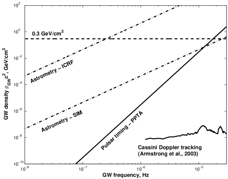
Figure 1: Astrometric (dot-dashed) and pulsar timing (solid) constraints on the overall energy density of a stationary isotropic background of monochromatic GWs as a function of the frequency $\nu$ in the range $\sim 10^{-8}\,\mathrm{Hz}<\nu<\sim 3\times 10^{-5}\,\mathrm{Hz}$ allowed by binary pulsar GW emission and DM clustering constraints (see Introduction). The thick dashed line corresponds to the local DM energy density of $0.3\,\mathrm{GeV}\mathrm{cm}^{-3}$. The constraint in the lower right corner of the graph is set by the Doppler tracking of the Cassini spacecraft armstrong:2003 .

III Astrometric constraints

The astrometric effect is different for the light propagating across a region of space with enhanced density of massive gravitons, e.g. a dark halo of a galaxy or galaxy cluster (the en-route effect), and for stochastic change of the position of the observer immersed in the massive graviton halo (the local effect). The former smears out the visible size of a distant source, while the latter changes stochastically the angular separation between different sources on the sky.

In astrophysically relevant cases the en-route effect is too small to be detected at the present level of accuracy of astrometric measurements. A very generous upper limit on the stochastically fluctuating change in the observed position of a distant source may be estimated as $\sigma_{\Psi}\sim h_{\mathrm{max}}\Psi_{\mathrm{L}}$, where $\Psi_{\mathrm{L}}$ is the angular size of the halo on the line of sight and $h_{\mathrm{max}}$ is the maximum amplitude of GWs comprising the halo (which, due to the Gaussian nature of these fluctuations, is essentially the same as the rms amplitude $h_{c}=\sqrt{P_{h}}$ that can be estimated from the dark matter density).

Contrary to naive expectations, in GR the light ray deflection does not execute a random walk and does not show the $\sim\sqrt{N}$ growth of the deflection. Instead, for traceless tensor perturbations travelling with the speed of light, only the gravitational wave field at emission and detection points matter Braginskyetal1990 ; kaiser:1997 ; Linder1986 . The relative change $\Delta\Psi/\Psi$ in the angular separation between two sources due to the local effect is also of order of the GW background amplitude $h_{c}$. At $h_{c}\sim 10^{-11}-10^{-10}$, as Dubovsky et al. model suggests dtt:2005 , this would yield $\sim\mathrm{\mu as}$ jitter in the angular separation for a couple of sources across the sky. Such jitter can be discovered in the future astrometric space experiments like SIM Shao (1992).

Present-day astrometric accuracy $\sigma_{\Psi}$ can be estimated as that of the radio VLBI-based ICRF (International Cosmic Reference Frame) Ma:1998 ; Fey:2004 , which involves more than 200 reference radio sources determining the celestial coordinate frame. The ICRF sources are observed for many years, and the accuracy of determination of source coordinates on the sky relative to this frame may be used as a measure of the angular separation stability. The best present-day accuracy of $100\,\mathrm{\mu as}$ (at $1\,\sigma$ level) Zharov:2008 means $\Delta\Psi\leq 5\times 10^{-10}$.

For the adopted power spectrum (3), this accuracy translates into the following upper limit on the GW mass density (see Appendix B):

$$\rho_{\mathrm{GW}}\leq\frac{3\pi\nu^{2}\sigma_{\Psi}^{2}}{4G}\hskip 142.26378pt$$ (7)

$$\approx 4.2\times 10^{3}\,\mathrm{GeV}\cdot\mathrm{cm}^{-3}\left(\frac{\nu}{3\times 10^{-5}\,\mathrm{Hz}}\right)^{2}\left(\frac{\sigma_{\Psi}}{100\,\mathrm{\mu as}}\right)^{2}.$$

Other limits for this value as a function of frequency $\nu$ are summarized on Fig. 1.

IV Conclusions

We have shown that the existing data on the millisecond pulsar timing stability set a tight upper limit on the narrow-band GW background amplitude at frequencies $\nu\leq 10^{-5}\mathrm{Hz}$. This limit can be used to severely bound the amount of massive cold gravitons which can potentially produce a strong narrow-band GW background dtt:2005 .

The present-day astrometric constraints are less restrictive than the timing ones at considered frequencies. However, both are still far above the tightest constraint set by the Doppler tracking of Solar system spacecrafts in the frequency range $\nu>10^{-6}\,\mathrm{Hz}$ armstrong:2003 .

Appendix A Pulsar timing in narrow-band GW background

To calculate the effect of a narrow-band GW background on pulsar timing one can use the formalism presented in Baskaran et al. deepak1:2008 starting with their expression (9), which describes the effect of a GW with wavevector $\bf{\tilde{k}^{\prime}}$ and polarization tensor $p_{ij}$ on the observed rotational frequency $f$ of a pulsar at position $\hat{\bf e}$ on the sky. Frequency fluctuation due to modes with all $s$ and ${\bf k}^{\prime}$ is

$$\Delta f(t)/f=\int\mathrm{d}{\bf k}^{\prime}\,\left[h_{s}({\bf k}^{\prime},t)g^{s}(p_{ij},\hat{\bf k}^{\prime},\hat{\bf e})+\mathrm{c.c.}\right],$$ (8)

where $g(p_{ij},\hat{\bf e},\hat{\bf k}^{\prime})$ is given by (9) of deepak1:2008 (setting the parameter $\epsilon\to 0$) and depends on the relative orientation of $\hat{\bf e},\hat{\bf k}^{\prime}$ and choice of the polarization gauge; in the above formula, summation of circulary polarized modes $s=1,2$ is implied and ‘c.c.’ stands for the complex conjugate.

The time of arrival residual $R(t)$ is the integral of relative fluctuation $\Delta f(t)/f$ w.r.t. time:

$$R(t)=\int\limits_{0}^{t}\mathrm{d}t\Delta f(t)/f$$ (9)

and its autocorrelation function is

$$R_{2}(\tau)\equiv\lim\limits_{T\to\infty}T^{-1}\int\limits_{0}^{T}\mathrm{d}t\,R(t)R(t+\tau).$$ (10)

In particular, plugging the above expressions into each other and using statistical properties of $h_{s}({\bf k},t)$ as set by Eq. (18) of deepak1:2008 one obtains for the ToA residual rms

$$r^{2}=R_{2}(0)=(3c^{2})^{-1}\int\mathrm{d}k^{\prime}\,P_{h}(k^{\prime})k^{\prime-3}$$ (11)

Applied to the power spectrum (3), this imediately gives

$$P_{0}\delta k=3r^{2}k^{3}c^{2}$$ (12)

and corresponding limit (6) on the GW mass density.

Appendix B Astrometric fluctuations in narrow-band GW background

To calculate the fluctuation $\Delta{\bf n}$ in the position of a source $\hat{\bf n}$ we write the astrometric effect due to a single GW mode in the formalism of deepak1:2008 similarly to Appendix A:

$$\Delta{\bf n}(t)={\bf f}^{s}(\hat{\bf k},\hat{\bf n})h_{s}({\bf k},t)+\mathrm{c.c.},$$ (13)

where conventions following (8) are respected and factors ${\bf f}^{s}(\hat{\bf{k}},\hat{\bf{n}})$ can be found by appropriately rotating the results of Pyne et al. PyneGwinnetal1996 :

$${\bf f}^{1,2}(\hat{\bf{k}},\hat{\bf{n}})=\frac{1}{2}\left\{\left[\hat{\bf n},\left[\hat{\bf k},\hat{\bf n}\right]\right]\pm i\left[\hat{\bf n},\hat{\bf k}\right]\right\}.$$ (14)

As $\Delta{\bf n}\perp\hat{\bf n}$, the former has only two independent components. For a pair of sources $\hat{\bf n},\hat{\bf n}^{\prime}$ it is natural to choose these components to be along the great circle connecting the pair and perpendicular to it. Using the above formulae and the statistical properties of $h_{s}({\bf k},t)$ as introduced in Eq. (18) of deepak1:2008 one obtains for the correlation matrix

$$\left(\begin{matrix}\Delta n^{\parallel}(\hat{\bf n},t)\Delta n^{\parallel}(\hat{\bf n}^{\prime},t^{\prime})&\Delta n^{\parallel}(\hat{\bf n},t)\Delta n^{\perp}(\hat{\bf n}^{\prime},t^{\prime})\cr\Delta n^{\perp}(\hat{\bf n},t)\Delta n^{\parallel}(\hat{\bf n}^{\prime},t^{\prime})&\Delta n^{\perp}(\hat{\bf n},t)\Delta n^{\perp}(\hat{\bf n}^{\prime},t^{\prime})\end{matrix}\right)=\hskip 14.22636pt$$ (15)

$$=\frac{1}{6}\left(\begin{matrix}1&0\cr 0&1\end{matrix}\right)\cos^{2}\frac{\Psi}{2}P_{c}(\tau)+\frac{1}{6}\left(\begin{matrix}1&0\cr 0&-1\end{matrix}\right)\sin^{2}\frac{\Psi}{2}P_{c}(2T)$$

where $\Psi=\angle(\hat{\bf n},\hat{\bf n}^{\prime})$, $\tau=t^{\prime}-t$, $2T=t^{\prime}+t$ and $P_{c}(t)$ is the cosine Fourier transform of the GW power spectrum $P_{h}$ (as defined by Eq. (18) of deepak1:2008 ):

$$P_{c}(t)\equiv\int\mathrm{d}k\,k^{-1}P_{h}(k)\cos{ckt};$$ (16)

for a $\delta$-like power spectrum (3), $P_{c}(t)=k^{-1}P_{0}\delta k\cos{ckt}$.

The autocorrelation function of the principal observable, the fluctuation $\Delta\Psi$ is

$$\left\langle\Delta\Psi\left(t\right)\Delta\Psi\left(t^{\prime}\right)\right\rangle=\frac{1}{3}\sin^{2}\frac{\Psi}{2}\left[P_{c}(\tau)-P_{c}(2T)\right].$$ (17)

Independent observations average away the second term in the square brackets above in accord with the stationarity of the problem. In particular, the rms value ($\tau=0$) in this case is

$$\left\langle\Delta\Psi^{2}\right\rangle=\frac{1}{3}\sin^{2}\frac{\Psi}{2}P_{c}(0)=\frac{P_{0}\delta k}{3k}\sin^{2}\frac{\Psi}{2};$$ (18)

hence the estimate (7).

The gravitational wave field is Gaussian and so is its linear transform $\Delta\Psi(t)$ (cf. 13). Therefore (15) readily gives the respective distribution functions. The results generalize naturally to multiple observables. For a set of $m$ angular distances $\Psi_{i}(t_{i})=\Psi_{i}+\Delta\Psi_{i}(t_{i})$ between source pairs $(\hat{\bf k}_{i},\hat{\bf n}_{i})$, the probability density $\varphi(\Delta{\boldsymbol{\Psi}})$ of the observable vector

$$\Delta{\boldsymbol{\Psi}}\equiv\left(\Delta\Psi_{1}(t_{1}),...,\Delta\Psi_{m-1}(t_{m-1}),\Delta\Psi_{m}(t_{m})\right)^{\mathrm{T}}$$

is

$$\varphi(\Delta{\boldsymbol{\Psi}})=\frac{\exp\left[-\frac{1}{2}\Delta{\boldsymbol{\Psi}}^{\mathrm{T}}\textbf{{M}}^{-1}\left(\hat{\bf n}_{1},...,\hat{\bf k}_{m};t_{1},...,t_{m}\right)\Delta{\boldsymbol{\Psi}}\right]}{\sqrt{(2\pi)^{m}\det\textbf{{M}}}}$$

with elements of M given by ($\Phi_{ij}=\angle(\hat{\bf n}_{i}+\hat{\bf k}_{i},\hat{\bf n}_{j}+\hat{\bf k}_{j})$):

$$M_{ij}=\frac{1}{3}\sin\frac{\Psi_{i}}{2}\sin\frac{\Psi_{j}}{2}\cos\Phi_{ij}P_{c}(t_{i}-t_{j}).$$

References

- (1) S. L. Dubovsky, P. G. Tinyakov, and I. I. Tkachev, Phys. Rev. Lett. 94, 181102 (2005a), eprint hep-th/0411158.
- (2) E. Komatsu et al., eprint arXiv:0803.0547 (2008)
- (3) G. Hinshaw et al., eprint arXiv:0803.0732 (2008)
- Milgrom (1983) M. Milgrom, Astrophys. J. 270, 371 (1983).
- Bekenstein (2004) J. D. Bekenstein, Phys. Rev. D70, 083509 (2004), eprint astro-ph/0403694.
- Gregory et al. (2000) R. Gregory, V. A. Rubakov, and S. M. Sibiryakov, Phys. Rev. Lett. 84, 5928 (2000), eprint hep-th/0002072.
- Dvali et al. (2000) G. R. Dvali, G. Gabadadze, and M. Porrati, Phys. Lett. B485, 208 (2000), eprint hep-th/0005016.
- Carroll et al. (2004) S. M. Carroll, V. Duvvuri, M. Trodden, and M. S. Turner, Phys. Rev. D70, 043528 (2004), eprint astro-ph/0306438.
- Kogan et al. (2001) I. I. Kogan, S. Mouslopoulos, and A. Papazoglou, Phys. Lett. B501, 140 (2001), eprint hep-th/0011141.
- Damour and Kogan (2002) T. Damour and I. I. Kogan, Phys. Rev. D66, 104024 (2002), eprint hep-th/0206042.
- Arkani-Hamed et al. (2004) N. Arkani-Hamed, H.-C. Cheng, M. A. Luty, and S. Mukohyama, JHEP 05, 074 (2004), eprint hep-th/0312099.
- Rubakov (2004) V. A. Rubakov (2004), eprint hep-th/0407104.
- Dubovsky (2004) S. L. Dubovsky, JHEP 10, 076 (2004), eprint hep-th/0409124.
- (14) V. Rubakov, P. Tinyakov, eprint arXiv:0802.4379 (2008).
- (15) V. S. Berezinsky, A. V. Gurevich and K. P. Zybin, PhLB, 294, 221 (1992)
- (16) M.V. Sazhin, Soviet Astr. (AZh), 22, 36 (1978).
- (17) S. Detweiler, ApJ, 234, 1100 (1979).
- (18) N. Kaiser, A. Jaffe, ApJ, 484, 545 (1997)
- (19) S.M. Kopeikin, G. Schäfer, C.R. Gwinn, and T.M. Eubanks, Phys. Rev. D, 59, id 084023 (1999)
- (20) D. Lorimer, Living Rev. Relativity 8, (2005), 7. URL (cited on 15.03.2008): http://www.livingreviews.org/lrr-2005-7
- (21) R.N. Manchester, eprint arXiv:0710.5026 (2007) Rms timing residuals obtained based on one-hour observations over two-year data span; no corrections for dispersion measure variations were done.
- (22) F.A. Jenet, G.B. Hobbs, K.J. Lee, and R.M. Manchester, ApJ, 625, L123 (2005).
- (23) F.A. Jenet, G.B. Hobbs, van Straten, et al., ApJ, 653, 1571 (2006).
- (24) D. Baskaran, A. G. Polnarev, M. S. Pshirkov, K. A. Postnov, Phys. Rev. D, 78, id 044018 (2008)
- (25) J.W. Armstrong et al., ApJ, 599, 806 (2003). Although Armstrong et al. assumed an isotropic GW background with locally flat energy density spectrum within the bandwidth equal to the center frequency, , these amplitude constraints can be also applied to the monochromatic waves.
- (26) V. Braginsky, N. Kardashev, A. Polnarev, I. Novikov, 1990, Nuovo Cimento B, 105, 1141
- (27) E. V. Linder, Phys. Rev. D, 34, 1759 (1986)
- Shao (1992) M. Shao, Proc. SPIE 3350, 536 (1998).
- (29) C. Ma, E.F. Arias, T.M. Eubanks, et al., Astron. J. 116, 516 (1998).
- (30) A.L. Fey, C. Ma, E.F. Arias, et al., Astron. J. 127, 3587 (2004).
- (31) V.E. Zharov, private communication (2008)
- (32) T. Pyne, C. Gwinn, M. Birkinshaw, T.M. Eubanks, N. Matsakis, 1996, ApJ, 465, 566