Diffusion of a passive scalar by convective flows under parametric disorder

Abstract

We study transport of a weakly diffusive pollutant (a passive scalar) by thermoconvective flow in a fluid-saturated horizontal porous layer heated from below under frozen parametric disorder. In the presence of disorder (random frozen inhomogeneities of the heating or of macroscopic properties of the porous matrix), spatially localized flow patterns appear below the convective instability threshold of the system without disorder. Thermoconvective flows crucially effect the transport of a pollutant along the layer, especially when its molecular diffusion is weak. The effective (or eddy) diffusivity also allows to observe the transition from a set of localized currents to an almost everywhere intense “global” flow. We present results of numerical calculation of the effective diffusivity and discuss them in the context of localization of fluid currents and the transition to a “global” flow. Our numerical findings are in a good agreement with the analytical theory we develop for the limit of a small molecular diffusivity and sparse domains of localized currents. Though the results are obtained for a specific physical system, they are relevant for a broad variety of fluid dynamical systems.

Special Issue: Article preparation, IOP journals

The effect of localization in spatially extended linear systems subject to a frozen random spacial inhomogeneity of parameters is known as Anderson localization (AL). AL has been first discovered and discussed for quantum systems [1]. Later on, investigations were extended to diverse branches of classical and semiclassical physics: wave optics (e.g., [2]), acoustics (e.g., [3]), etc. The phenomenon has been comprehensively studied and well understood mathematically for the Schrödinger equation and related mathematical models (e.g., [4, 5, 6]). Also, the role of nonlinearity in these models has been addressed in the literature (for instance, destruction of AL by nonlinearity [7, 6]).

Being well studied for conservative media (or systems) the localization phenomenon did not receive a comparable attention for active/dissipative ones as, e.g., in problems of thermal convection or reaction-diffusion. The main reason is that the physical interpretations of formal solutions to the Schrödinger equation and governing equations for active/dissipative media are essentially different and, therefore, the theory of AL may be extended to the latter only under certain strong restrictions (this statement is discussed in details in the end of the next section). Nevertheless, effects similar to AL can be observed in fluid dynamical systems ([8]; in [9] the effect of parametric disorder on the excitation threshold in one-dimensional Ginzburg–Landau equation has been studied, but without attention to localization effects). In this paper, we study an example: the problem where localized thermoconvective currents excited under parametric disorder crucially influence the process of transport of a passive scalar (e.g., a pollutant).

The paper is organized as follows. In section 1 we formulate the specific physical problem we deal with, introduce the relevant mathematical model, and discuss physical background for the problem. Section 2 presents the results of a numerical simulation. In section 3 we develop an analytical theory for a certain limit case. Section 4 ends the paper with conclusions.

1 Problem formulation and basic equations

The modified Kuramoto–Sivashinsky equation

$$\dot{\theta}(x,t)=-\left(\theta_{xxx}(x,t)+q(x)\,\theta_{x}(x,t)-(\theta_{x}(x,t))^{3}\right)_{x}$$ (1)

is relevant for a broad variety of active media where pattern selection occurs. It governs two-dimensional (2D) large-scale natural thermal convection in a horizontal fluid layer heated from below [10, 11] and holds valid for a turbulent fluid [12], a binary mixture at small Lewis number [13], a porous layer saturated with a fluid [14, 8], etc. Specifically, in the problems mentioned, temperature perturbations $\theta$ are almost uniform along the vertical coordinate $z$ and obey (1).

To argue for a general validity of (1), let us note the following. Basic laws in physics are the conservation ones. This fact quite often results in final equations having the form $\partial_{t}[\mbox{quantity}]+\nabla\!\cdot\![\mbox{flux of quantity}]=0$. With such conservation laws either for systems with the sign inversion symmetry of the fields, which is wide spread in physics, or for description of a spatiotemporal modulation of an oscillatory mode, the original Kuramoto–Sivashinsky equation (e.g., see [15]) should be rewritten in the form (1). On these grounds, we claim equation (1) to describe pattern formation in a broad variety of physical systems.

In the following we restrict our consideration to the case of convection in a porous medium; nevertheless, the most of results may be easily extended to the other physical systems mentioned. Equation (1) is already dimensionless and below we introduce all parameters and variables in appropriate dimensionless forms.

Recall, the large-scale (or long-wavelength) approximation is identical to the approximation of a thin layer and assumes that the characteristic horizontal scales are large against the layer height $h$. For large-scale convection, $(21/2)h^{2}q(x)$ (cf. (1), [14]) represents relative deviations of the heating intensity and of the macroscopic properties of the porous matrix (porosity, permeability, heat diffusivity, etc.) from the critical values for the spatially homogeneous case. Thus, for positive spatially uniform $q$, convection sets up, while for negative $q$, all the temperature inhomogeneities decay. For convection in a porous medium [14], the macroscopic fluid velocity field

$$\vec{v}=\frac{\partial\Psi}{\partial z}\vec{e}_{x}-\frac{\partial\Psi}{\partial x}\vec{e}_{z}\,,\qquad\Psi=\frac{3\sqrt{35}}{h^{3}}\,z(h-z)\,\theta_{x}(x,t)\equiv f(z)\,\psi(x,t)\,,$$ (2)

where $\psi(x,t)\equiv\theta_{x}(x,t)$ is the stream function amplitude, the reference frame is such that $z=0$ and $z=h$ are the lower and upper boundaries of the layer, respectively (figure 1b). Though the temperature perturbations obey (1) for diverse convective systems, function $f(z)$, which determines the relation between the flow pattern and the temperature perturbation, is specific for each case.

(a)
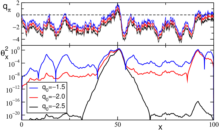
(b)

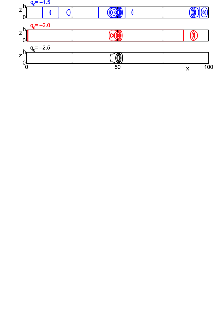
Figure 1: (a): Establishing steady solutions to (1) for $q_{0}$ indicated in the plot are sets of exponentially localized patterns [shown for one and the same realization of random inhomogeneity $\xi(x)$ and $\varepsilon=1$; $q(x)$ is represented by $q_{\pi}(x)=\pi^{-1}\int_{x-\pi/2}^{x+\pi/2}q(x^{\prime})\rmd x^{\prime}$]. (b): The stream lines corresponding to the solutions in graph (a) are plotted for the case of convection in a porous layer [cf. (2)].

Though (1) is valid for a large-scale inhomogeneity $q(x)$, which means $h|q_{x}|/|q|\ll 1$, one may set such a hierarchy of small parameters, namely $h\ll(h|q_{x}|/|q|)^{2}\ll 1$, that a frozen random inhomogeneity may be represented by white Gaussian noise $\xi(x)$:

$$q(x)=q_{0}+\xi(x),\quad\left\langle\xi(x)\right\rangle=0,\quad\left\langle\xi(x)\xi(x^{\prime})\right\rangle=2\varepsilon^{2}\delta(x-x^{\prime}),$$

where $\varepsilon^{2}$ is the disorder intensity and $q_{0}$ is the mean supercriticality (i.e. departure from the instability threshold of the disorderless system). Numerical simulation reveals only steady solutions to establish in (1) with such $q(x)$ [8].

Let us now discuss some general points related to the physical problem under consideration. Obviously, the linearized form of equation (1) in the stationary case, i.e.,

$$-\theta_{xxx}(x)-\xi(x)\,\theta_{x}(x)=q_{0}\,\theta_{x}(x)\,,$$

is a stationary Schrödinger equation for $\psi=\theta_{x}$ with $q_{0}$ instead of the state energy and $-\xi(x)$ instead of the potential. Therefore, like for the Schrödinger equation (e.g., see [4, 5, 6]), all the solutions $\psi(x)$ to the stationary linearized equation (1) are spatially localized for arbitrary $q_{0}$; asymptotically,

$$\psi(x)\propto\exp(-\gamma|x|),$$

where $\gamma$ is the localization exponent. Such a localization can be easily seen for a solution to the nonlinear problem (1) in figure 1a for $q_{0}=-2.5$.

One should keep in mind, that, in the quantum Schrödinger equation, localized modes are bound states of, e.g., an electron in a disordered media. Even the mutual nonlinear interaction of these modes, which appears due to the electron–electron interaction and leads to destruction of AL, should be interpreted in the context of the specific physical meaning of the quantum wave function. Therefore, the theory developed for AL in quantum systems may not be directly extended to active/dissipative media. Indeed, in (1), all excited localized modes of the linearized problem do mutually interact via nonlinearity in a way where they irreversibly lose their identity (unlike solitons in soliton bearing systems, which completely recover after mutual collision). Thus, when the spatial density of excited localized modes is large and these modes form an almost everywhere intense flow, localization properties of formal solutions to the linearized problem do absolutely not manifest themselves.

Nevertheless, when excited modes are spatially sparse, solitary exponentially localized patterns can be discriminated as reported in [8]. Figure 1 shows sample patterns for such a case. One can see that for negative $q_{0}$ the spatial density of excited modes rapidly decreases as $q_{0}$ decreases and the pattern localization becomes more pronounced. For a small spatial density of excited modes, one can distinguish all these modes and introduce the observable quantifier $\nu$ of the established steady pattern, which measures the spatial density of the domains of excitation of convective flow; fortunately, an empiric formula fits perfectly the numerically calculated dependence [8],

$$\nu\approx\frac{1}{4\sqrt{1.95\,\pi}\,\varepsilon^{2/3}|\widetilde{q}_{0}|}\exp\left(-\frac{1.95\,\widetilde{q}_{0}^{2}}{4}\right),$$ (3)

where $\widetilde{q}_{0}\equiv\varepsilon^{-4/3}q_{0}$.

Here we would like to emphasize the fact of existence of convective currents below the instability threshold of the disorderless system. These currents may considerably and nontrivially affect transport of a pollutant (or other passive scalar), especially when its molecular diffusivity is small (for instance, for microorganisms or suspensions the diffusion due to Brownian motion is drastically weak against the possible convective transport). Transport of a nearly indiffusive passive scalar is the subject of our research, as a “substance” which is essentially influenced by these localized currents and, thus, provides an opportunity to observe manifestation of disorder-induced phenomena discussed in [8].

From the viewpoint of mathematical physics, there is one more nontrivial question which is worthy to be addressed. In AL an important topological effect takes place; while in 1D case all the solutions are localized, in higher dimensions spatially unbounded solutions appear (e.g., [4]). The modification of (1) for the case of inhomogeneity in the both horizontal directions, $q=q(x,y)$, (e.g., see [14]) cannot be turned into the Schrödinger equation even after linearization in the stationary case. Thus, there are no reasons for any topological effects directly analogous to the one mentioned for AL. Nevertheless, one may speak of a percolation kind transition, where the domain of an intense convective flow becomes globally connected for high enough $q_{0}$. Noteworthy, this transition cannot be observed in 1D system (1) as there is always a finite probability of a large domain of negative $q(x)$ where the flow is damped and the domain of an intense flow becomes disconnected. Essentially, the flow damped never decays exactly to zero and, hence, one needs a formal quantitative criterion for the absence of intense currents at a certain point. On the other hand, this transition leads to a crucial enhancement of transport of a nearly indiffusive scalar along the layer, and the intensity of this transport can be used to detect the transition immediately in the context that arises applied interest to it. In this way, one also avoids introducing a formal quantitative criterion. Remarkably, in the context of transport of a passive scalar, that is the subject of the study we present, the transition from a set of spatially localized currents to an almost everywhere intense “global” flow can be observed in 1D system (1) as well.

Let us describe the transport of a passive (i.e., not influencing the flow in contrast, for instance, to [16]) pollutant by a steady convective flow (2). The flux $\vec{j}$ of the pollutant concentration $C$ is

$$\vec{j}=\vec{v}\,C-D\nabla C\,,$$ (4)

where the first term describes the convective transport and the second one represents the molecular diffusion, $D$ is the molecular diffusivity. The establishing steady distributions of the pollutant obey

$$\nabla\cdot\vec{j}=0\,.$$ (5)

Equation (5) yields a uniform along $z$ distribution of $C$ (see appendix),

$$\frac{\rmd C(x)}{\rmd x}=-\frac{J}{\displaystyle D+\frac{21\,\psi^{2}(x)}{2h^{2}D}}\,,$$ (6)

where $J$ is the constant pollutant flux along the layer. Note, for the other convective systems we mentioned above, the result differs only in the factor ahead of $\psi^{2}/D$.

2 Effective diffusivity

In this section we introduce and consider the effective diffusivity (for general ideas on introducing the effective diffusivity one can consult, e.g., [17, 18]). Let us consider the domain $x\in[0,L]$ with the imposed concentration difference $\delta C$ at the ends. Then the establishing pollutant flux $J$ is defined by the integral [cf. (6)],

$$\delta C=-J\int\limits_{0}^{L}\frac{\rmd x}{\displaystyle D+\frac{21\,\psi^{2}(x)}{2h^{2}D}}\,.$$

For a lengthy domain the specific realization of $\xi(x)$ becomes insignificant;

$$\delta C=-J\,L\left\langle\left(D+\frac{21\,\psi^{2}(x)}{2h^{2}D}\right)^{-1}\right\rangle\equiv-\sigma^{-1}J\,L\,,$$

Hence,

$$J=-\sigma\frac{\delta C}{L},$$

i.e. $\sigma$ can be considered as an effective diffusivity.

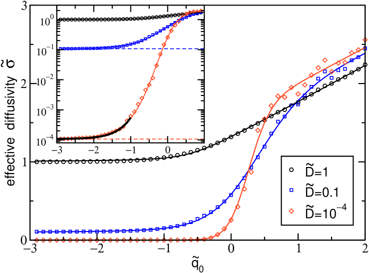
Figure 2: Dependencies of effective diffusivity $\sigma$ on mean supercriticality $q_{0}$ for molecular diffusivity $D$ indicated in the plot. The bold black line in the inner plot represents the analytical dependence (see section 3).

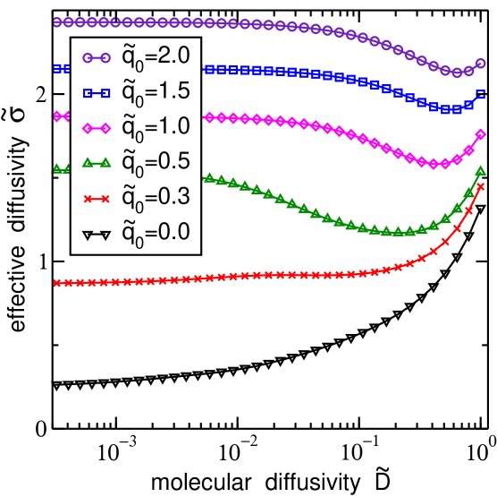
Figure 3: Dependencies of the effective diffusivity on the molecular one for nonnegative $\widetilde{q}_{0}$

The effective diffusivity

$$\sigma=\left\langle\left(D+\frac{21\,\psi^{2}(x)}{2h^{2}D}\right)^{-1}\right\rangle^{-1}$$ (7)

turns into $D$ for vanishing convective flow. For small $D$ the regions of the layer, where the flow is damped, $\psi\ll 1$, make large contribution to the mean value appearing in (7) and diminish $\sigma$, thus, leading to the locking of the spreading of the pollutant.

Note, disorder strength $\varepsilon^{2}$ can be excluded from equations by the appropriate rescaling of parameters and fields. Thus, the results on the effective diffusivity can be comprehensively presented in the terms of $\widetilde{D}$, $\widetilde{\sigma}$, and $\widetilde{q}_{0}$:

$$\widetilde{D}=\sqrt{\frac{2}{21}}\,\varepsilon^{4/3}hD,\qquad\widetilde{\sigma}=\sqrt{\frac{2}{21}}\,\varepsilon^{4/3}h\sigma,\qquad\widetilde{q}_{0}=\frac{q_{0}}{\varepsilon^{4/3}}\,.$$

Figure 2 provides calculated dependencies of effective diffusivity $\widetilde{\sigma}$ on $\widetilde{q}_{0}$ for moderate and small values of molecular diffusivity $\widetilde{D}$. Noteworthy,
(i) for small $\widetilde{D}$ a quite sharp transition of effective diffusivity $\widetilde{\sigma}$ between moderate values and ones comparable with $\widetilde{D}$ occurs near $q_{0}=0$, suggesting the transition from an almost everywhere intense “global” flow to a set of localized currents to take place;
(ii) below the instability threshold of the disorderless system, where only sparse localized currents are excited, the effective diffusion can be dramatically enhanced by these currents; e.g., for $\widetilde{D}=10^{-4}$, $\widetilde{q}_{0}=-1$, the effective diffusivity is increased by one order of magnitude compared to the molecular diffusivity.

Figure 3 shows dependencies of the effective diffusivity on the molecular one for nonnegative $q_{0}$. Remarkably, for $\widetilde{q}_{0}\gtrsim 0.3$, the dependencies possess a minimum which is in agreement with known general results on interference between turbulent and molecular diffusion [19]. The reason is the fact, that for the convective transport the molecular diffusion plays a destructive role. Hence, for high $q_{0}$, where convective flows are intense, the enhancement of the convective transport prevails over the weakening of the diffusional one as the molecular diffusivity tends to zero; on the contrary, for low $q_{0}$, where convective flows are weak, the decrease of the molecular diffusivity leads to the weakening of the transport.

3 Analytical theory

Let us now analytically evaluate the effective diffusivity for a small molecular one, $\widetilde{D}\ll 1$, and sparse domains of excitation of convective flow, $\nu\ll 1$. We have to calculate the average

$$\beta\equiv\left\langle\big{(}\widetilde{D}+\psi^{2}(x)/\widetilde{D}\big{)}^{-1}\right\rangle$$

[cf. (7)] which, due to ergodicity, can be evaluated not only as an average over $x$ for a given realization of $\xi(x)$, but also as an average over realizations of $\xi(x)$ at a certain point $x_{0}$. Let us set the origin of the $x$-axis at $x_{0}$. Hence, $\beta=\langle\big{(}\widetilde{D}+\psi^{2}(0)/\widetilde{D}\big{)}^{-1}\rangle_{\xi}$.

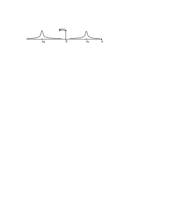
Figure 4: Sketch of two localized flow patterns being nearest to the origin

When the two nearest to the origin excitation domains are distant and localized near $x_{1}>0$ and $x_{2}<0$ (see figure 4),

$$\psi(0)\approx\psi_{1}\rme^{-\gamma x_{1}}+\psi_{2}\rme^{-\gamma|x_{2}|},$$ (8)

where $\psi_{1,2}$ characterize the amplitude of flows excited around $x_{1,2}$. For small $\widetilde{D}$ and density $\nu$, the contribution of the excitation domains to $\beta$ is negligible against the one of the regions of a weak flow. Therefore, we do not have to be very accurate with the former and may utilize expression (8) even for small $x_{1,2}$,

$$\beta=\left\langle\frac{1}{\widetilde{D}+\psi^{2}(0)/\widetilde{D}}\right\rangle_{\xi}$$

$$\qquad=\left\langle\int\limits_{0}^{\infty}\rmd x_{1}\int\limits_{0}^{\infty}\rmd x_{2}\frac{p(x_{1})\,p(x_{2})}{\widetilde{D}+\widetilde{D}^{-1}(\psi_{1}\rme^{-\gamma x_{1}}+\psi_{2}\rme^{-\gamma x_{2}})^{2}}\right\rangle_{\psi_{1},\psi_{2}}$$ (9)

where $p(x_{1})$ [ $p(x_{2})$] is the density of the probability to observe the nearest right [left] excitation domain at $+x_{1}$ [$-x_{2}$]. For probability distribution $P(x_{1}\!>\!x)$, one finds $P(x_{1}\!>\!x+\rmd x)=P(x_{1}\!>\!x)\,(1-\nu\rmd x)$, i.e., $\frac{\rmd}{\rmd x}P(x_{1}\!>\!x)=-\nu P(x_{1}\!>\!x)$. Hence, $P(x_{1}\!>\!x)=\rme^{-\nu x}$, and probability density $p(x)=|\frac{\rmd}{\rmd x}P(x_{1}\!>\!x)|=\nu\rme^{-\nu x}$. With regard to averaging over $\psi_{1,2}$, it is important that the multiplication of $\psi_{1,2}$ by factor $F$ is effectively equivalent to the shift of the excitation domain by $\gamma^{-1}\ln{F}$ which is insignificant for $F\sim 1$ in the limit case we consider. Hence, one can assume $\psi_{1,2}=\pm 1$ (the topological difference between $\psi_{1}\psi_{2}<0$ and $\psi_{1}\psi_{2}>0$ is not to be neglected) and rewrite (9) as

$$\beta=\frac{1}{2}\int\limits_{0}^{\infty}\rmd x_{1}\int\limits_{0}^{\infty}\rmd x_{2}\,\nu^{2}\rme^{-\nu(x_{1}+x_{2})}\left[\frac{1}{\widetilde{D}+\widetilde{D}^{-1}(\rme^{-\gamma x_{1}}+\rme^{-\gamma x_{2}})^{2}}\right.$$

$$\hskip 199.16928pt\left.{}+\frac{1}{\widetilde{D}+\widetilde{D}^{-1}(\rme^{-\gamma x_{1}}-\rme^{-\gamma x_{2}})^{2}}\right].$$

These integrals can be evaluated for $\nu/\gamma\ll 1$, and one finds

$$\widetilde{\sigma}=\frac{1}{\beta}\approx\widetilde{D}\left(\frac{2}{\widetilde{D}}\right)^{\frac{2\nu}{\gamma}}\!\!.$$ (10)

For $\widetilde{q}_{0}\!<\!-1$, one can use the asymptotic expressions for $\nu$ [equation (3)] and

$$\gamma=\varepsilon^{-\frac{2}{3}}\left(|\widetilde{q}_{0}|^{\frac{1}{2}}-\frac{1}{4}|\widetilde{q}_{0}|^{-1}-\frac{5}{32}|\widetilde{q}_{0}|^{-\frac{5}{2}}+\dots\right).$$

The latter expression is known from the classical theory of AL (cf. [5, 6]).

In figure 2, one can see analytic expression (10) to match the numerically evaluated $\widetilde{\sigma}$ for $\widetilde{D}=10^{-4}$, $\widetilde{q}_{0}\!<\!-1$ quite well. With (10), one can evaluate the convectional enhancement of the effective diffusivity below the excitation threshold of the disorderless system, and it is given by factor $\widetilde{\sigma}/\widetilde{D}=(2/\widetilde{D})^{2\nu/\gamma}$ which can be large for small $\widetilde{D}$.

4 Conclusion

Summarizing, we have studied the transport of a pollutant in a horizontal fluid layer by spatially localized 2D thermoconvective currents appearing under frozen parametric disorder. Though the specific physical system we have considered is a horizontal porous layer saturated with a fluid and confined between two nearly thermally insulating plates, our results can be trivially extended to a broad variety of fluid dynamical systems (like ones studied in [10, 11, 12, 13]). We have calculated numerically the dependence of the effective diffusivity on the molecular one and the mean supercriticality (see figures 2, 3). In particular, for a nearly indiffusive pollutant ($\widetilde{D}\ll 1$), first, we have observed the transition from a set of localized flow patterns to an almost everywhere intense “global” flow, which results in a soar of the effective diffusivity from values comparable with the molecular diffusivity up to moderate ones. Second, we have found convective currents to considerably enhance the effective diffusivity even below this transition. For the latter effect the analytical theory, which perfectly describes the limit of $\widetilde{D}\ll 1$, $\nu\ll 1$, has been developed [equation (10)].

Appendix: Diffusion by stationary flow

The following derivation of equation (6) is performed in the spirit of the standard multiscale method (interested readers can consult, e.g., [20, 18]). We consider the transport of a pollutant in a layer with boundaries impermeable both for the fluid and for the pollutant. In order to derive (6), we substitute filtration velocity $\vec{v}$ from (2) and pollutant flux $\vec{j}$ from (4) into conservation law (5), and write down

$$(\Psi_{z}C)_{x}-(\Psi_{x}C)_{z}-D(C_{xx}+C_{zz})=0$$ (11)

(the subscripts $x$ and $z$ indicate respective derivatives). The absence of the fluxes of the pollutant and the fluid trough the boundary, ı.e., $j^{z}(z\!=\!0)=j^{z}(z\!=\!h)=0$ and $v^{z}(z\!=\!0)=v^{z}(z\!=\!h)=0$ (the superscripts $x$ and $z$ indicate the respective components of vectors), results in boundary conditions

$$z=0,\,h:\quad C_{z}=0\,.$$ (12)

We assume $D\sim h^{-1}$, and use $h$ as a small parameter of expansion; $\partial_{z}\propto h^{-1}\!$, $D=h^{-1}D_{-1}$, $f(z)=h^{-1}f_{-1}(z)$, $C(x,z)=C_{0}(x,y)+h\,C_{1}(x,y)+h^{2}C_{2}(x,y)+...$ . Then (11) reads

$$\begin{array}[]{l}h^{-1}\partial_{x}[f_{-1,z}\theta_{x}(C_{0}+h\,C_{1}+...)]-h^{-1}\partial_{z}[f_{-1}\theta_{xx}(C_{0}+h\,C_{1}+...)]\\[8.0pt] -h^{-1}D_{-1}[C_{0,xx}\!+C_{0,zz}\!+h(C_{1,xx}\!+C_{1,zz})+h^{2}(C_{2,xx}\!+C_{2,zz})\!+...]=0.\end{array}$$ (13)

From (13) in the order $h^{-3}$:

$$-C_{0,zz}=0\,.$$

Due to boundary conditions (12), $C_{0,z}=0$, i.e., in the leading order the concentration is uniform along $z$,

$$C_{0}=\eta_{0}(x)\,.$$

From (13) in the order $h^{-2}$:

$$\partial_{x}[f_{-1,z}\theta_{x}C_{0}]-\partial_{z}[f_{-1}\theta_{xx}C_{0}]-h\,D_{-1}C_{1,zz}=0\,,$$

i.e.,

$$C_{1,zz}=(h\,D_{-1})^{-1}f_{-1,z}(z)\,\theta_{x}(x)\,\eta_{0,x}(x)\,.$$

The last equation yields

$$C_{1}=g_{1}(z)\eta_{1}(x)+A(x)z+B(x)\,,$$

where

$$g_{1,zz}=h^{-1}f_{-1,z}=3\sqrt{35}\,(h-2z)/h^{3},\quad\eta_{1}(x)=D_{-1}^{-1}\,\theta_{x}(x)\,\eta_{0,x}(x)\,.$$

Formally, $g_{1}=3\sqrt{35}(z^{2}/2h^{2}-z^{3}/3h^{3}+az+b)$. Boundary conditions (12) result in $A(x)=a=0$; $B(x)$ makes a uniform along $z$ contribution to $C$, like $\eta_{0}(x)$, and, therefore, can be treated as a part of $\eta_{0}$. Hence, we may claim $\int_{0}^{1}C_{1}\rmd z=0$, i.e., $B(x)=b=0$, and obtain

$$C_{1}=g_{1}(z)\,\eta_{1}(x)=3\sqrt{35}\left(\frac{z^{2}}{2h^{2}}-\frac{z^{3}}{3h^{3}}\right)\eta_{1}(x)\,.$$

Let us now find the gross pollutant flux $h\,J$ through a vertical cross-section of the layer. The integral of $j^{x}$ [equation (4)] over $z$ is

$$h\,J \equiv \int\limits_{0}^{h}j^{x}\rmd z=\int\limits_{0}^{h}(v^{x}C-DC_{x})\rmd z=\int\limits_{0}^{h}(\Psi_{z}C-DC_{x})\rmd z$$

$$= \int\limits_{0}^{h}(f_{z}\theta_{x}C-DC_{x})\rmd z=\int\limits_{0}^{h}(f_{z}\theta_{x}\eta_{0}+h\,f_{z}g_{1}\theta_{x}\eta_{1}-D\eta_{0,x}+O(h^{3}))\rmd z$$

$$\approx h\,\theta_{x}\eta_{1}\int\limits_{0}^{h}f_{z}g_{1}\,\rmd z-h\,D\eta_{0,x}=-h\left(\frac{21}{2h^{2}D}(\theta_{x})^{2}\eta_{0,x}+D\eta_{0,x}\right).$$

As the pollutant is not accumulated anywhere, flux $J$ should be constant along the layer. Hence, we find equation (6) providing the relation between the concentration field and the flux.

References

References

- [1] Anderson P W 1958 Phys. Rev.109 1492–505
- [2] van Rossum M C W and Nieuwenhuizen Th M 1999 Rev. Mod. Phys.71 313–71
- [3] Maynard J D 2001 Rev. Mod. Phys.73 401–17
- [4] Fröhlich J and Spencer T 1984 Phys. Rep. 103 9–25
- [5] Lifshitz I M, Gredeskul S A and Pastur L A 1988 Introduction to the Theory of Disordered Systems (New York: Wiley).
- [6] Gredeskul S A and Kivshar Yu S 1992 Phys. Rep. 216 1–61
- [7] Pikovsky A S and Shepelyansky D L 2008 Phys. Rev. Lett.100 094101
- [8] Goldobin D S and Shklyaeva E V 2008 Localization and advectional spreading of convective flows under parametric disorder Phys. Rev.E submitted [preview: arXiv:0804.3741]
- [9] Hammele M, Schuler S and Zimmermann W 2006 Physica D 218 139–57
- [10] Knobloch E 1990 Physica D 41 450–79
- [11] Shtilman L and Sivashinsky G 1991 Physica D 52 477–88
- [12] Aristov S N and Frik P G 1989 Fluid Dynamics 24(5) 690–5
- [13] Schöpf W and Zimmermann W 1989 Europhys. Lett. 8 41–6 Schöpf W and Zimmermann W 1993 Phys. Rev.E 47 1739–64
- [14] Goldobin D S and Shklyaeva E V 2008 Large-scale thermal convection in a horizontal porous layer Phys. Rev.E submitted [preview: arXiv:0804.2825]
- [15] Michelson D 1986 Physica D 19 89–111
- [16] Goldobin D S and Lyubimov D V 2007 JETP 104 830–6
- [17] Frisch U 1995 Turbulence: The Legacy of A. N. Kolmogorov (Cambridge: Cambridge University Press) p 226
- [18] Majda A J and Kramer P R 1999 Phys. Rep. 314 238–574
- [19] Saffman P G 1960 J. Fluid. Mech. 8 273–83 Mazzino A and Vergassola M 1997 Europhys. Lett. 37 535–40
- [20] Bensoussan A, Lions J L and Papanicolaou G 1978 Asymptotic Analysis for Periodic Structures (Amsterdam: North-Holland)