Two-Dimensional Hydrodynamic Models of Super Star Clusters with a Positive Star Formation Feedback

Abstract

Using the hydrodynamic code ZEUS, we perform 2D simulations to determine the fate of the gas ejected by massive stars within super star clusters. It turns out that the outcome depends mainly on the mass and radius of the cluster. In the case of less massive clusters, a hot high velocity ($\sim 1000$ km s^-1) stationary wind develops and the metals injected by supernovae are dispersed to large distances from the cluster. On the other hand, the density of the thermalized ejecta within massive and compact clusters is sufficiently large as to immediately provoke the onset of thermal instabilities. These deplete, particularly in the central densest regions, the pressure and the pressure gradient required to establish a stationary wind, and instead the thermally unstable parcels of gas are rapidly compressed, by a plethora of re-pressurizing shocks, into compact high density condensations. Most of these are unable to leave the cluster volume and thus accumulate to eventually feed further generations of star formation.

The simulations cover an important fraction of the parameter-space, which allows us to estimate the fraction of the reinserted gas which accumulates within the cluster and the fraction that leaves the cluster as a function of the cluster mechanical luminosity, the cluster size and heating efficiency.

1 Introduction

Due to their stellar mass, which in some cases amounts to several million M_⊙, and their compactness, as they only span a few parsecs, young ($<10$ Myr) super star clusters (SSCs) represent the most spectacular and dominant mode of star formation in starburst and interacting galaxies (O’Connell et al., 1995; Ho, 1997; Whitmore & Schweizer, 1995; Melo et al., 2005). SSCs have been detected in the optical, UV and X-rays, and also in the radio continuum and IR regimes, as some of them are deeply embedded behind dense obscuring material, leading to powerful ultra-dense HII regions (Kobulnicky & Johnson, 1999; Gilbert & Graham, 2007).

On theoretical grounds, it has been inferred that such extreme modes of star formation should lead to several tens of thousands of massive stars, all of them known to rapidly ($\leq 50$ Myr) reinsert, through stellar winds and supernova (SN) explosions, a large fraction of their mass back into the ISM. The first (adiabatic) approach to the hydrodynamics of the matter reinserted within a SSC is due to Chevalier & Clegg (1985, hereafter CC85). In their model, the stellar sources of mass and energy, are assumed to be equally spaced within the SSC volume of radius $R_{\mathrm{SC}}$. They also assumed that all of the kinetic energy provided by massive stars is immediately, and in situ, thermalized via random collisions of the ejecta from neighboring sources. This results in energy and mass deposition rate densities $q_{e}=(3L_{\mathrm{SC}})/(4\pi R_{\mathrm{SC}}^{3})$ and $q_{m}=(3\dot{M}_{\mathrm{SC}})/(4\pi R_{\mathrm{SC}}^{3})$, respectively, where $L_{\mathrm{SC}}$ and $\dot{M}_{\mathrm{SC}}$ are the cluster mechanical luminosity and mass deposition rates. These assumptions lead to a high temperatures gas ($T>10^{7}$ K) in which the interstellar cooling law is close to its minimum value, and this justifies their adiabatic assumption. In the adiabatic model of CC85, the thermalized hot gas rapidly settles into almost constant density and temperature distributions, although a slight outward pressure gradient establishes a particular velocity distribution with the stagnation point (i.e. zero velocity) at the cluster center. The gas velocity increases then almost linearly with radius to reach the sound speed ($c_{\mathrm{SC}}$) right at the cluster surface and then streams into the surrounding lower pressure ambient medium to reach its terminal velocity ($v_{\mathrm{A\infty}}\sim 2c_{\mathrm{SC}}$), while the density and temperature of the outflow, the cluster wind, decrease as $r^{-2}$ and $r^{-4/3}$, respectively. The solution of such a stationary outflow depends on three variables: the cluster size ($R_{\mathrm{SC}}$), the mass deposition rate ($\dot{M}_{\mathrm{SC}}$) and the mechanical luminosity of the cluster ($L_{\mathrm{SC}}$). Knowledge of these three variables allows one to solve the hydrodynamic equations analytically and workout the run of density, temperature and velocity of the stationary outflow. Note that $\dot{M}_{\mathrm{SC}}$ is usually replaced by the adiabatic terminal speed ($v_{\mathrm{A\infty}}=(2L_{\mathrm{SC}}/\dot{M}_{\mathrm{SC}})^{1/2}$).

The model then yields a stationary flow in which the matter reinserted by the evolving massive stars ($\dot{M}_{\mathrm{SC}}$) equals the amount of matter feeding the cluster wind ($4\pi R_{\mathrm{SC}}^{2}\rho_{\mathrm{SC}}c_{\mathrm{SC}}$); where $\rho_{\mathrm{SC}}$ is the reinserted gas density value at the star cluster surface. As $L_{\mathrm{SC}}$ and $\dot{M}_{\mathrm{SC}}$ increase linearly with the cluster mass ($L_{\mathrm{SC}}\sim M_{\mathrm{SC}}$, $\dot{M}_{\mathrm{SC}}\sim M_{\mathrm{SC}}$), the adiabatic model predicts that the more massive a cluster is, the more powerful is its resultant wind. This latter conclusion breaks down if one relaxes the adiabatic assumption (see Silich et al., 2004). More massive clusters deposit larger amounts of matter and thereby deliver a sufficiently high density, $\rho_{\mathrm{SC}}=\dot{M}_{\mathrm{SC}}/(4\pi R_{\mathrm{SC}}^{2})$, to provoke strong radiative cooling. Thus, as radiative cooling ($Q$ = $n^{2}\Lambda(T,Z)$; where $\Lambda(T,Z)$ is the cooling function) is proportional to $M_{\mathrm{SC}}^{2}$ and $L_{\mathrm{SC}}$ is proportional to $M_{\mathrm{SC}}$, there is a threshold mechanical luminosity (for given $R_{\mathrm{SC}}$ and $\dot{M}_{\mathrm{SC}}$), above which strong radiative cooling takes over despite the large temperatures and the minimum value of the interstellar cooling law at these temperatures.

Note that details of the thermalization process have been largely ignored although more recent formulations of the problem (Wünsch et al., 2007; Silich et al., 2007) have inferred that a significant fraction of the deposited mechanical energy could be radiated away as soon as it is inserted. In such cases, only a fraction of the deposited energy remains available to heat the thermalized matter. This fraction is called the heating efficiency, $\eta$. It is assumed by different authors to have values between $0.01$ and $1$ (Bradamante et al., 1998; Melioli & de Gouveia Dal Pino, 2004), and shown to acquire small values in the case of massive compact SSCs (see Silich et al., 2007).

Figure 1 presents the threshold mechanical luminosity found by Silich et al. (2004), here re-calculated for three different values of the heating efficiency $\eta$. Clusters with a mechanical luminosity (or mass) far below this line evolve in the quasi-adiabatic regime. For these, the Chevalier & Clegg model provides a good approximation to the structure and hydrodynamics of the star cluster wind (Cantó et al., 2000; Raga et al., 2001). Figure 2 displays radial profiles of temperature, particle density, pressure and velocity, typical of such steady state winds.

For clusters with a mechanical luminosity close to the threshold value, the temperature distribution within the stationary wind becomes very different from that predicted by the adiabatic model (Silich et al., 2004). This is because, as soon as the temperature of the wind decreases to approximately $\sim 10^{6}$ K, radiative cooling begins to increase sharply (mainly due to f-b and b-b transitions of heavy elements) and the temperature in the free wind region drops rapidly several orders of magnitude. Nevertheless such clusters manage to eject all the matter deposited by stellar winds and supernovae, and thereby sustain a stationary wind.

For clusters above the threshold line, radiative cooling becomes a dominant factor. Radiative cooling affects first the central densest regions causing a sudden drop in pressure. This promotes the shift of the stagnation point out of the cluster center. Such clusters adhere to a bimodal solution (Tenorio-Tagle et al., 2007; Wünsch et al., 2007) in which the stagnation radius ($R_{\mathrm{st}}$) defines two different regions within the cluster volume (see Figure 3). On one hand, there is an outer shell in which the deposited energy, although affected by strong radiative cooling, is still able to drive an outward stationary wind, by making the gas velocity acquire the sound speed exactly at the cluster surface. On the other hand, the matter deposited inside the stagnation radius is strongly affected by radiative cooling and becomes thermally unstable. The instability leads to a rapid and continuous loss of energy from large and small parcels of gas, thereby reducing their temperature and pressure. These events lead immediately to the formation of strong shocks that emanate from the hot, high pressure regions and are driven into the cold parcels of gas in order to restore their pressure. These have been termed re-pressurizing shocks, and have been invoked in several astrophysical circumstances, such as the formation of globular clusters (Vietri & Pesce, 1995), and also in the cooling of supernova matter within superbubbles, leading to highly metallic droplets falling onto the galaxy (Tenorio-Tagle, 1996). In the context of the matter cooling inside the superstar cluster stagnation radius, the re-pressurizing shocks have been first modelled by means of 1D numerical hydrodynamics in Tenorio-Tagle et al. (2007). The re-pressurizing shocks rapidly compress the cold gas, enhancing its density while reducing its volume, until the cold condensations acquire again the thermal pressure value of the hot gas. Given the initially similar values of density ahead of and behind the shocks, one can show that their velocity is only a function of the temperature $T$ of the hot gas ($V_{\mathrm{RP}}\approx[(kT)/(\mu m_{p})]^{0.5}$, where $k$ is the Boltzmann constant, $\mu m_{p}$ is the mean gas-particle mass, and $m_{p}$ is the proton mass), and thus cold parcels of gas within the SSC are rapidly driven into small high density condensations.

The continuous occurrence of thermal instabilities results in the accumulation of mass in this region and in a very chaotic, highly non-stationary hydrodynamical pattern, with a number of radiative shocks and cooling fronts propagating within the cluster volume. The continuous accumulation of thermally unstable matter must finally lead to its re-processing into further generations of stars (Tenorio-Tagle et al., 2005). Unfortunately, 1D simulations do not allow one to reach an adequate understanding of the physics within massive clusters in the bimodal regime, nor to make realistic predictions regarding the fate of the matter reinserted by massive stars. In order to develop a more realistic model, here we present detailed 2D hydrodynamic simulations of the gaseous flows that result from the thermalization of the kinetic energy supplied by stellar winds and supernovae ejecta inside the volume occupied by the stellar cluster. We focus on clusters evolving in the bimodal regime. The major result from these simulations is that the central zones of clusters evolving in the bimodal regime accumulate large amounts of matter in the form of warm ($T\sim 10^{4}$ K) high density condensations embedded into a hot plasma of much lower density. The amount of accumulated matter depends on the excess star cluster mechanical luminosity over the threshold value and grows with time, unless the accumulation of reinserted matter inside the stagnation radius is compensated by secondary star formation. Our results also show that the stagnation surface itself has a very complicated dynamic morphology that continuously changes with time. Nevertheless, the average radius of the stagnation surface remains close to that predicted by 1D and semi-analytic calculations.

The paper is organized as follows. Section 2 describes the numerical model and discusses the input physics. Section 3 present the results from our numerical simulations and compares them with the semi-analytical results and previous 1D simulations. In section 4 we discuss our results and section 5 gives a summary of our findings.

Figure 1: The threshold lines. Clusters above the threshold line evolve in a bimodal regime in which the injected matter is accumulated inside their densest inner regions while the outer zones develop a strongly radiative stationary wind. The threshold lines were calculated for the adiabatic terminal velocity $V_{\mathrm{A\infty}}=1000$ km s^-1 and three different heating efficiencies $\eta=1.0,0.3$ and $0.1$ denoted with solid, dashed and dotted lines, respectively. The 2D simulations (see Table 1) are represented by symbols. Different symbols denote different heating efficiencies (and thus are to be compared with the corresponding threshold line) $\eta=1.0$ (triangles), $\eta=0.3$ (circles), and $\eta=0.1$ (plus signs). The secondary y-axis shows the approximate mass of the cluster obtained using a relation $M_{\mathrm{SC}}=(L_{\mathrm{SC}}/3\times 10^{40})10^{6}$ M_⊙ (Leitherer et al., 1999).

Figure 2: Model 1 ($L_{\mathrm{SC}}/L_{\mathrm{crit}}=0.5$): radial profiles of the wind particle density, $n_{w}$ (note the units are $m^{-3}$ to fit within the figure), temperature ($T_{w}$), pressure ($P_{w}$) and radial velocity ($v_{w}$). The thin lines represent the semi-analytical solution (Silich et al., 2004), the thick lines are results from the 2D simulation (model 1) at $t=0.25$ Myr. The simulation, after a short initial relaxation period, stays perfectly stationary and spherically symmetric at all times.

Figure 3: The internal structure of SSCs in the bimodal regime. The cluster volume presents two distinct regions. Below the stagnation radius $R_{\mathrm{st}}$: is the thermally unstable region and above it lies the outer quasi-stationary wind region. The radial profiles of the wind particle density, temperature, pressure and radial velocity were obtained as the axial time averages values of the 2D simulation (model 3) between $0.4$ and $0.8$ Myr. Only the hot gas ($T>2\times 10^{4}$) was taken into consideration for this plot. The values of temperature and pressure at the stagnation radius, obtained from the semi-analytical model (thin solid lines across the inner region), are given with horizontal lines.

2 The numerical approach

The numerical models presented here are based on the finite difference Eulerian hydrodynamic code ZEUD3D v3.4.2 (Stone & Norman, 1992). All simulations have been carried out on a spherical ($r$, $\theta$) grid, symmetric along the $\phi$-coordinate. We have set the radial size of grid cells $\Delta r$ proportional to the radial coordinate $r$ which ensures that all grid-cells have $\Delta r\sim r\Delta\theta$. Another advantage of this radially scaled grid is that the resolution is higher at smaller radii (inside the cluster) where thermal instabilities are expected.

The cooling routine accounts for extremely fast cooling both in the wind or within the SSC volume. The change of internal energy $e$ due to cooling is

$$\left.\frac{de}{dt}\right|_{\mathrm{cool}}=-n_{i}n_{e}\Lambda(T,Z)\ ,$$ (1)

where $n_{i}$ and $n_{e}$ are ion and electron densities, respectively. We compute them from the gas density $\rho$ as $n_{i}=n_{e}=\rho/(\mu_{\mathrm{ion}}m_{p})$, where $\mu_{\mathrm{ion}}m_{p}$ is the average ion mass. We assume $\mu=0.609$ and $\mu_{\mathrm{ion}}=1.27$ for all computed models. $\Lambda(T,Z)$ is the cooling function. We use Raymond & Cox cooling function which has been supplemented with new elements and tabulated by Plewa (1995).

The RHS of equation (1) is evaluated in the middle of time-steps to maintain the second order accuracy of the code and the energy conservation equation is then solved iteratively using the Brendt algorithm which is more stable and accurate than the Newton-Raphson method originally used in ZEUS.

The cooling rate has to be included in the computation of the time-step, otherwise rapid cooling not resolved in time may lead to the occurrence of negative temperatures. A common way of solving this is to limit the amount of internal energy which can be radiated away during one time-step by setting

$$dt_{\mathrm{cool}}=\epsilon\left|\frac{e}{\left.\frac{de}{dt}\right|_{\mathrm{cool}}}\right|$$ (2)

where $\epsilon$ is a safety factor smaller than unity (see e.g. Suttner et al. 1997; where $\epsilon=0.3$ was used). In this work we use $\epsilon=0.25$.

The global time-step, $dt$, is computed as follows:

$$dt=\left\{\begin{array}[]{lcl}dt=dt_{\mathrm{HD}},&\mathrm{for}&dt_{\mathrm{cool}}\geq dt_{\mathrm{HD}};\\ dt=dt_{\mathrm{cool}},&\mathrm{for}&dt_{\mathrm{HD}}>dt_{\mathrm{cool}}\geq\delta\times dt_{\mathrm{HD}};\\ dt=\delta\times dt_{\mathrm{HD}},&\mathrm{for}&\delta\times dt_{\mathrm{HD}}>dt_{\mathrm{cool}}\ (\mathrm{local\ substeps}\ dt_{\mathrm{sub}}=dt_{\mathrm{cool}});\end{array}\right.$$ (3)

where $dt_{\mathrm{HD}}$ is the ”hydrodynamic” time-step resulting from the Courant-Friedrich-Levi criterion and $\delta$ is the minimum fraction of $dt_{\mathrm{HD}}$ to which the global time-step $dt$ is allowed to drop. If, due to the cooling condition, a certain cell requires an even smaller time-step (i.e. $dt_{\mathrm{cool}}<\delta dt_{\mathrm{HD}}$), the energy equation is integrated numerically in that cell, using $dt_{\mathrm{sub}}=dt_{\mathrm{cool}}$ but assuming that during this time the density and temperature in the cell are not substantially affected by interactions with neighboring cells. This ensures that CPU time is not wasted in cells where a high time resolution is not required. To determine a reasonable value of $\delta$ we ran several tests on a low resolution grid ($150\times 56$) and found that there are no appreciable differences for $\delta\lesssim 0.3$. Therefore, we use $\delta=0.1$.

In order to simulate the effect of the stellar UV radiation field, in some of the simulations (see Table 1), we do not allow the gas temperature to drop below $T_{\mathrm{lim}}=10^{4}$ K. This is equivalent to assuming that there are sufficient UV photons to ionize the dense thermally unstable matter which otherwise would cool to much lower temperatures.

The wind source was modelled by a continuous replenishment of mass and internal energy in all cells within the cluster volume, at rates $q_{m}=(3\dot{M}_{\mathrm{SC}})/(4\pi R_{\mathrm{SC}}^{3})$ and $q_{e}=(3\dot{L}_{\mathrm{SC}})/(4\pi R_{\mathrm{SC}}^{3})$, respectively. The procedure applied to each cell within the cluster volume at every time-step is:

1. the density and the total energy in a given cell are saved to $\rho_{\mathrm{old}}$ and $e_{\mathrm{tot,old}}$

2. the new mass is inserted $\rho_{\mathrm{new}}=\rho_{\mathrm{old}}+(1+A_{\mathrm{noise}}\zeta)q_{\mathrm{m}}dt$, the velocity is corrected so that the momentum is conserved $\mathbf{v}_{\mathrm{new}}=\mathbf{v}_{\mathrm{old}}\rho_{\mathrm{old}}/\rho_{\mathrm{new}}$

3. the internal energy is corrected to conserve the total energy $e_{\mathrm{i,mid}}=e_{\mathrm{tot,old}}-\rho_{\mathrm{new}}\mathbf{v}^{2}_{\mathrm{new}}/2$

4. the new energy is inserted in a form of internal energy $e_{\mathrm{i,new}}=e_{\mathrm{i,mid}}+(1+A_{\mathrm{noise}}\zeta)q_{\mathrm{e}}dt$

where $\zeta$ is a pseudo-random number from the interval $(-1,1)$ generated each time it is used, and $A_{\mathrm{noise}}$ is the relative amplitude of the noise. The inclusion of a noise term is necessary to break the artificial spherical symmetry imposed by the initial conditions (see below). The model is very robust with respect to $A_{\mathrm{noise}}$. Test runs with $A_{\mathrm{noise}}=0.01,0.05,0.1$ and $0.5$ lead to very similar general properties (mass fluxes at boundaries, number of fragments formed and their approximate sizes) in all models. The only noticeable difference is the duration of the initial relaxation period required to break the initial symmetry. We use $A_{\mathrm{noise}}=0.1$ for all models described in this paper.

The boundary conditions are set open at both r-boundaries and periodic at both $\theta$-boundaries. The open inner r-boundary allows the dense clumps that are not ejected from the cluster (through its boundary at $R_{\mathrm{SC}}$) to leave the computational domain. Otherwise, they would accumulate within the cluster and eventually fill its whole volume; this happens for some models with high $L_{\mathrm{SC}}$ and low $\eta$, even with the open inner r-boundary (see Section 3.5). It is unphysical, because the accumulated mass exceeds the amount which can be ionized by the available UV photons; therefore it should cool down, become gravitationally unstable and collapse into stars. Moreover, the accumulated mass ultimately becomes so high that it would be gravitationally unstable even at $T=10^{4}$ K. However, determining the fate of the dense mass properly would need a model of star formation which takes into account radiation transfer and self-gravity: this is not included in our current numerical model.

Two different initial conditions are used for the two series of models presented here (see Table 1). Models 1 – 6 and 12 with $R_{\mathrm{SC}}=10$ pc have as initial condition the spherically symmetric semi-analytical solution with $L_{\mathrm{SC}}=L_{\mathrm{crit}}$ (Silich et al., 2004). Models 7 - 11 and 13, with $R_{\mathrm{SC}}=3$ pc, use as initial condition the semi-analytical solution with the appropriate $L_{\mathrm{SC}}$. As this is only fully defined for $r>R_{\mathrm{st}}$, at $t=0$ the central region $r<R_{\mathrm{st}}$ is filled with a zero velocity, constant density and temperature gas, with values equal to those at the stagnation radius $\rho=\rho(R_{\mathrm{st}})$ and $T=T(R_{\mathrm{st}})$, respectively. The advantage of this approach is that such conditions are closer to the quasi-stationary state and therefore it takes a shorter time to reach it.

3 Results

We have calculated two series of models (see Table 1). Models in the first series all have a cluster radius $R_{\mathrm{SC}}=10$ pc and an assumed heating efficiency $\eta=1$. The cluster mechanical luminosities considered are: $2.5\times 10^{41}$, $10^{42}$, $10^{43}$ and $10^{44}$ erg s^-1, which result in values of $L_{\mathrm{SC}}/L_{\mathrm{crit}}=0.5$, $2$, $20$ and $200$, respectively. The model with $L_{\mathrm{SC}}/L_{\mathrm{crit}}=2$ was computed with three different numerical resolutions $150\times 56$, $300\times 112$ and $600\times 224$ to check and establish convergence. The computational domain extents radially from $R_{\mathrm{IB}}=2$ pc (the inner boundary) to $R_{\mathrm{OB}}=30$ pc (the outer boundary) and from $\theta_{\mathrm{LB}}=\pi/2-0.5$ (left boundary) to $\theta_{\mathrm{RB}}=\pi/2+0.5$ (right boundary) in the axial direction.

For the second series of models, we assume a more compact cluster and more realistic cluster parameters by setting $R_{\mathrm{SC}}=3$ pc and $\eta=0.1$ or $0.3$. We ran 6 models with 3 different ratios $L_{\mathrm{SC}}/L_{\mathrm{crit}}=2.5$, $25$ and $250$. In these cases the radial extent of the grid goes from $R_{\mathrm{IB}}=0.5$ pc to $R_{\mathrm{OB}}=10$ pc, and the axial extent goes from $\pi/3$ to $2\pi/3$.

In all cases we assumed an adiabatic terminal velocity is $v_{\mathrm{A,\infty}}\equiv\sqrt{\frac{2L_{\mathrm{SC}}}{\dot{M}_{\mathrm{SC}}}}=1000$ km/s, and the lower temperature limit was set equal to $T_{\mathrm{lim}}=10^{4}$ K, or 10² K (models 12 and 13). In cases with an $\eta<1$, $v_{\mathrm{A,\infty}}$, was replaced by $v_{\mathrm{A,\infty}}\equiv\sqrt{\frac{2\eta L_{\mathrm{SC}}}{\dot{M}_{\mathrm{SC}}}}$. Note that in all cases, radiative cooling lowers the outflow velocity at the grid outer boundary to somewhat smaller values.

No.	$\frac{L_{\mathrm{SC}}}{\mathrm{[erg/s]}}$	$\frac{R_{\mathrm{SC}}}{\mathrm{[pc]}}$	$\eta$	$\frac{L_{\mathrm{SC}}}{L_{\mathrm{crit}}}$	grid	$T_{\mathrm{lim}}$	$\frac{R_{\mathrm{st}}}{\mathrm{[pc]}}$	$\frac{T_{\mathrm{st}}}{\mathrm{[}10^{6}\mathrm{K]}}$	$\frac{\dot{M}_{\mathrm{out}}}{\dot{M}_{\mathrm{SC}}}$	$T_{\mathrm{min}}$
1	$2.5\times 10^{41}$	10	1	0.5	$300\times 112$	$10^{4}$	0	$10.4$	1.00	$10^{4}$
2	$10^{42}$	10	1	2	$150\times 56$	$10^{4}$	6.056	$10.4$	0.81	$10^{4}$
3	$10^{42}$	10	1	2	$300\times 112$	$10^{4}$	6.056	$10.4$	0.84	$10^{4}$
4	$10^{42}$	10	1	2	$600\times 224$	$10^{4}$	6.056	$10.4$	0.79	$10^{4}$
5	$10^{43}$	10	1	20	$300\times 112$	$10^{4}$	8.991	$10.4$	0.39	$10^{4}$
6	$10^{44}$	10	1	200	$300\times 112$	$10^{4}$	9.696	$10.4$	0.19	$10^{4}$
7	$10^{39}$	3	0.1	2.5	$300\times 104$	$10^{4}$	1.872	$1.10$	0.77	$10^{4}$
8	$10^{40}$	3	0.3	2.5	$300\times 104$	$10^{4}$	1.860	$3.48$	0.84	$10^{4}$
9	$10^{40}$	3	0.1	25	$300\times 104$	$10^{4}$	2.709	$1.10$	0.98	$10^{4}$
10	$10^{41}$	3	0.3	25	$300\times 104$	$10^{4}$	2.707	$3.48$	0.83	$10^{4}$
11	$10^{41}$	3	0.1	250	$300\times 104$	$10^{4}$	2.912	$1.10$	1.00	$10^{4}$
12	$10^{43}$	10	1	20	$300\times 112$	$10^{2}$	8.991	$10.4$	0.38	$10^{2}$
13	$10^{40}$	3	0.1	25	$300\times 104$	$10^{2}$	2.709	$1.10$	0.44	$10^{2}$

Table 1: The set of computed models. The values of $R_{\mathrm{st}}$ and $T_{\mathrm{st}}$ were determined by means of semi-analytic models, the values of $\dot{M}_{\mathrm{out}}/\dot{M}_{\mathrm{SC}}$ are the mass flux through the cluster border in the 2D simulations, averaged over the time interval $0.1-0.8$ Myr for $R_{\mathrm{SC}}=10$ pc models and $1-2$ Myr for $R_{\mathrm{SC}}=3$ pc models.

3.1 Model 1, $L_{\mathrm{SC}}/L_{\mathrm{crit}}=0.5$

This model was computed in order to test the numerical code against the semi-analytical solution which is known for $L_{\mathrm{SC}}<L_{\mathrm{crit}}$. Despite the perturbations of the deposited mass and energy, the flow is perfectly stationary. The resultant radial density, temperature and velocity profiles are shown in Figure 2 where they are compared to the semi-analytic solution. The agreement is very good, despite the fact that the 2-D model does not calculate the central sphere of radius $R_{\mathrm{IB}}$, and this induces a small discrepancy in the velocity in the inner cluster regions.

3.2 Model 5, $L_{\mathrm{SC}}/L_{\mathrm{crit}}=20$

We continue with a detailed description of model 5 which exhibits the typical hydrodynamic behavior for clusters above the threshold line, $L_{\mathrm{SC}}>L_{\mathrm{crit}}$. The model starts with the semi-analytical solution for $L_{\mathrm{SC}}=L_{\mathrm{crit}}$ and from then onwards, at each time step, the mass and energy input rates are consistent with the selected ratio $L_{\mathrm{SC}}/L_{\mathrm{crit}}=20$. Initially, the density grows slowly all over the cluster volume, and this steadily enhances the radiative cooling, causing lower temperatures. Eventually, as the temperature approaches $T\sim 3\times 10^{5}$ K, the cooling rate increases steeply, and thermal instability occurs. This lowers the temperature rapidly to $T=10^{4}$ K, particularly in the densest central regions. On the other hand, the outer regions, where the density is lower, remain hot and thus a large pressure gradient between the two regions leads to the formation of a strong shock wave propagating inwards (see Figure 4, left column).

The simulations show a very dynamic evolution in which regions of hot gas of different dimensions appear and grow close to the center, as more energy is deposited within the cluster volume. The hot gas expands super-sonically into the low pressure warm ($10^{4}$ K) surroundings. This decreases locally the density of the hot gas, preventing its becoming thermally unstable, while at the same time the parcels of warm gas are compressed from all sides into high density condensations, until they reach pressure equilibrium with the surrounding hot gas. The hot regions grow until they again occupy most of the cluster volume, see Figure 4, middle column.

While all this is happening, the inward propagating shock wave, overruns the central region, accelerating inwards most of the high density condensations, and these eventually leave the computational grid as they cross the inner boundary. As the high temperatures are reestablished, the overall pressure gradient vanishes and the shock wave decays. Once the hot gas again permeates the cluster volume, the density starts to grow again and the whole process repeats itself, but in a weaker form because of the presence of a few dense condensations surviving from the previous cycle. This model exhibits 2-3 subsequent weaker periods of oscillations similar to the ones observed in 1D simulations (Tenorio-Tagle et al. 2007; the low-energy model).

Finally, the oscillations vanish and a quasi-equilibrium situation is established, in which high density condensations form at an approximately constant rate (see Figure 4, right column). The amount of mass which goes into warm dense condensations is just enough to maintain the hot medium close to the thermally unstable regime. It is a quasi-stationary situation: the density tends to grow everywhere, surpassing some threshold value that favours the thermal instability in the densest central regions. This sudden loss of pressure prevents matter within the stagnation boundary from escaping the cluster as a wind. The thermally unstable gas is instead packed into high density condensations, most of which leave the computational grid through the inner boundary. The location of the stagnation surface, which separates the region where the thermal instability occurs from the outer stationary wind, also experiences some oscillations. This leads to a non-spherical surface with an average radius close to that given by the analytic approximation (Wünsch et al., 2007),

$$\frac{R_{\mathrm{st}}^{3}}{R_{\mathrm{SC}}^{3}}=1-\left(\frac{L_{\mathrm{crit}}}{L_{\mathrm{SC}}}\right)^{1/2}\ .$$ (4)

The $R_{\mathrm{st}}$ radius at which vicinity the orientation of the velocity vectors abruptly changes from an outward to an inward motion has been indicated with a red line in the bottom panels of Figure 4.

3.3 Models 2-4, $L_{\mathrm{SC}}/L_{\mathrm{crit}}=2$

In these cases the stagnation radius $R_{\mathrm{st}}$ is smaller than in model 5, resulting in a smaller thermally unstable region. The lower mass deposition rate results in a smaller amount of high density gas being formed there (see Figure 5). Otherwise, the evolution is similar to that of model 5, including the initial relaxation period of intense thermal instability, the appearance of re-pressurizing shocks which lead to high density condensations, and the exit of most of these through the inner boundary, to finally reach equilibrium between the formation of high density condensations and the mass deposition rate.

We have computed this model on three different grids to check how the resolution affects the results (see the different rows of Figure 5). Although the resultant fragments tend to be smaller and more structured on the higher resolution grids, the global characteristics such as the mass flux through the cluster border (see Table 1) are in a reasonable agreement.

3.4 Model 6, $L_{\mathrm{SC}}/L_{\mathrm{crit}}=200$

The hydrodynamical behavior of this case is very similar to that of model 5, the only differences are quantitative: In this case many more high density condensations form and occupy a larger fraction of the cluster volume (see Figure 6). The quasi-stationary region, above the rapidly varying stagnation surface, becomes at times very narrow and, as it is repeatedly perturbed by high density condensations leaving the cluster, at times it is not even a contiguous region. Nevertheless, most of the thermally unstable gas driven into high density condensations stays within the cluster volume and after some time, as in model 5, goes through the inner boundary and disappears from the computational domain.

3.5 Other Models

The most important parameter of our cluster model is the ratio $L_{\mathrm{SC}}/L_{\mathrm{crit}}$, as this defines the location of the stagnation surface and thus the relative sizes of the thermally unstable region and of the quasi-stationary outer wind region. We have performed many more simulations (see Table 1), all presenting the same general features as in model 5. For example models 7 and 8, ($L_{\mathrm{SC}}/L_{\mathrm{crit}}=2.5$, $\eta=0.1$ and $0.3$) have $L_{\mathrm{SC}}/L_{\mathrm{crit}}$ values close to those of models 2 - 4. However, the smaller heating efficiency $\eta$ assumed in these cases, results in a smaller temperature and pressure of the hot medium, and this leads to a stationary wind that expands with a smaller velocity. The lower temperature of the hot gas leads to slower velocity re-pressurizing shocks. The lower ambient pressure of the hot gas also leads to larger final sizes of the high density condensations and after some time to their accumulation near the central zones of the computational grid. This sooner or later prevents the exit of matter through the inner boundary in case of models 9 and 10 ($L_{\mathrm{SC}}/L_{\mathrm{crit}}=25$, $\eta=0.1$ and $0.3$) and model 11 ($L_{\mathrm{SC}}/L_{\mathrm{crit}}=250$, $\eta=0.1$). We believe this is an artifact promoted by the fact that we do not allow for this matter to go into star formation.

Models 12 and 13 are similar to models 5 and 9, respectively, but the gas is allowed to cool to $10^{2}$ K instead of $10^{4}$ K. A comparison between model 12 and 5 shows very similar results. This means that the reduced volume of clumps in model 12 (due to their lower temperature and hence pressure) does not affect the ratio of the clumps that are ejected from the cluster to the clumps that stay there and finally leave the computational domain through the inner boundary. Therefore, the outflow from the cluster ($\dot{M}_{\mathrm{out}}$) remains the same in both models. However, in the case of model 13 ($R_{\mathrm{SC}}=3$ pc, $\eta=0.1$), the reduction of the clump sizes prevents accumulating and filling the cluster with a dense warm material, as happens in model 9. As shown in Figure 7 and in Table 1 the formation of new clumps via thermal instability is compensated with the outflow from the computational zone making, model 13 more realistic.

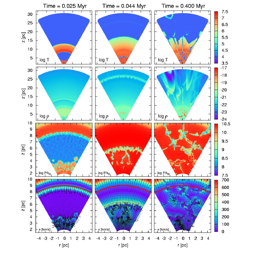
Figure 4: Model 5 ($L_{\mathrm{SC}}/L_{\mathrm{crit}}=20$, $\eta=1$) at $t=0.025$ Myr (left column), $t=0.044$ Myr (middle column) and $t=0.4$ Myr (right column). The first two rows of panels show the logarithm of the wind temperature and density, respectively, across the whole computational domain. The third row shows the logarithm of pressure in the cluster central region (below $R_{\mathrm{SC}}=10$ pc), and the bottom row shows the wind velocity in the same region, as arrows together with its magnitude coded by the color scale. The red arc is the stagnation radius given by the semi-analytical solution.

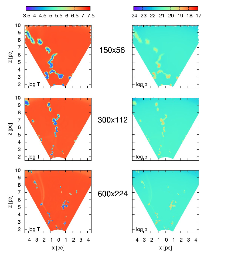
Figure 5: Models 2-4 ($L_{\mathrm{SC}}/L_{\mathrm{crit}}=2$, $\eta=1$) at $t=0.25$ Myr. The left and right columns show the logarithm of the wind temperature and density, respectively, in the cluster central region. The three rows of panels represent the different grid resolutions: the top row is $150\times 56$ (model 2), the middle row $300\times 112$ (model 3) and the bottom row $600\times 224$ (model 4).

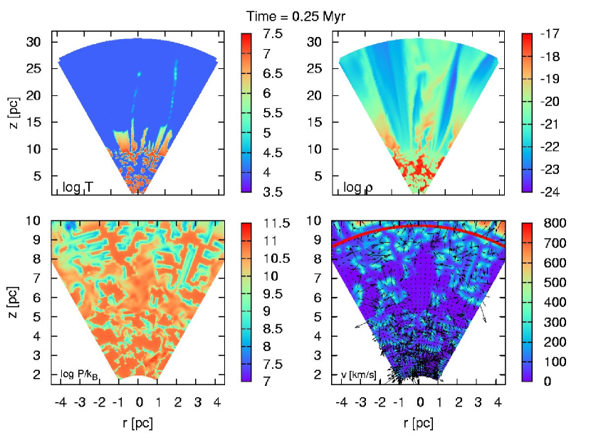
Figure 6: Model 6 ($L_{\mathrm{SC}}/L_{\mathrm{crit}}=200$, $\eta=1$) at $t=0.25$ Myr. The top left and right panels show the logarithm of the wind temperature and density, respectively, across the whole computational domain. The bottom panels show only the cluster region (below $R_{\mathrm{SC}}=10$ pc), the left panel represents the logarithm of pressure, the right panel shows the wind velocity as arrows together with its magnitude coded by the color scale. The red arc is the stagnation radius given by the semi-analytical solution.

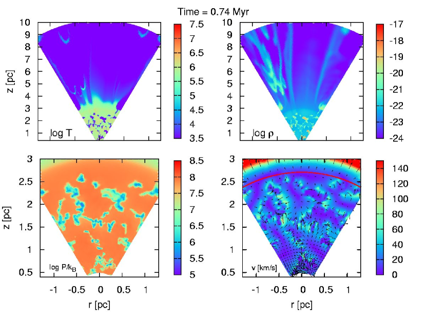
Figure 7: Model 13 ($L_{\mathrm{SC}}/L_{\mathrm{crit}}=25$, $\eta=0.1$) at $t=0.74$ Myr. The meaning of the panels is the same as in Figure 6.

Figure 8: The solid line represents the time evolution of the mass flux measured at the outer boundary of the computation domain in model 5. The mass deposition rate to the whole cluster $\dot{M}_{\mathrm{SC}}$ and its fraction deposited between $R_{\mathrm{st}}$ and $R_{\mathrm{SC}}$ are represented by dash-dotted line and dashed line, respectively. The dotted line represents the average flux at the outer boundary in the period 0.2 - 0.8 Myr. Those average mass fluxes are shown as symbols in Figure 9. The rarefied wind produces the flux close to the value given by the dashed line. The maxima of $\dot{M}_{\mathrm{out}}$ are due to condensations passing through the outer boundary. They are preceded by short periods in which $\dot{M}_{\mathrm{out}}$ drops below the dashed line, as if the condensations ”cast shadows” to the regions above them – the mass flux of the rarefied wind is slightly lower then and corresponds to the moments when the outer boundary is shadowed by an approaching condensation(s).

Figure 9: The fraction of the matter inserted within the stellar cluster which is able to leave it as a function of the cluster luminosity normalized by its threshold value ($L_{\mathrm{SC}}/L_{\mathrm{crit}}$). The solid line represents the fraction of mass which is inserted above $R_{\mathrm{st}}$ and which leaves the cluster in a form of the hot wind (which may eventually cool down outside the cluster). The $\times$ symbols denote the 1D simulations described in Tenorio-Tagle et al. (2007). The other symbols represent the 2D simulations: triangles (models 2 – 6), the plus (model 7), the circle (model 8), the square (model 12), and the diamond (model 13). The values were obtained by averaging over time periods $0.2-0.8$ Myr (models 2 – 6), and $1-2$ Myr (models 7, 8, 12 and 13). The dashed line is the fit to the outflows of 2D models.

4 Discussion

Figure 8 shows the time evolution of the mass flux through the outer boundary of the computational domain for model 5. The outflow becomes quasi-stationary as an equilibrium is established between the formation of high density condensations and their ejection from the cluster and exit through the inner boundary. The average mass flux across the outer boundary of the computation domain (dotted line in Figure 8) slightly exceeds the rate of mass deposition that occurs between the stagnation radius $R_{\mathrm{st}}$ and the star cluster edge $R_{\mathrm{SC}}$. This is because some dense condensations that formed in the thermally unstable inner region ($r<R_{\mathrm{st}}$) cross the stagnation surface and eventually leave the cluster contributing to the total mass flux across the outer boundary of the computational grid.

Figure 9 shows how the relative outflow from the cluster (measured as the mass flux at the outer boundary, averaged over long time periods) depends on the ratio $L_{\mathrm{SC}}/L_{\mathrm{crit}}$. We plot all the models where the equilibrium between the clump formation and their removal through inner or outer boundaries is reached. Other models (Nos 9, 10 and 11), where the volume of the cluster is completely filled with the warm matter (see Sect. 3.5.) are omitted. The outflow from the cluster consists of two components: the hot wind, which originates in the outer region of the cluster above $R_{\mathrm{st}}$, and the warm dense clumps that are formed below $R_{\mathrm{st}}$ and that manage to pass to the outer region where they are ejected from the cluster. The figure shows three zones: the bottom zone is the fraction of the deposited mass that goes into the wind, the middle zone represents the mass in ejected high density condensations that stream away with the wind ($\lesssim 20\%\dot{M}_{\mathrm{SC}}$), and the upper zone is the mass which stays in the cluster (available for star formation). Note that the hot wind also cools down to temperatures $T\sim 10^{4}$ K at short distances from the cluster surface, so, finally there are also two phases in the outflow: the warm wind and the dense condensations (which should expand unless they cool even further).

In order to advance the problem further, apart from an adequate hydrodynamic model that takes into consideration specific characteristics of SSCs (i.e. their high masses, small radii, large stellar densities and extreme output of mechanical energy), one would need to couple the hydrodynamics to the UV radiation field. We have assumed here that this is the case and that the UV radiation field generated by the massive stars evolving in the cluster keeps the temperature of the thermally unstable gas at $T\sim 10^{4}$ K through photoionization. This may be true for very young clusters, before the supernova era starts ($t_{\mathrm{SN}}\sim$3 Myr). However, older clusters, with a reduced ionizing photon flux, would soon become unable to photoionize all the gas that became thermally unstable. In such cases, (see Figure 7) the thermally unstable gas would continue to cool further, while being compressed into correspondingly smaller volumes. As a result, the increasingly high densities would trap the ionization front in the outer skins of the condensations and their interior would remain neutral and at low temperature ($\sim 10$ K). In this way, if a parcel of gas with an original temperature $\sim 10^{7}$ K, that becomes thermally unstable and is able to cool down to $10$ K, would experience a rapid evolution in which its volume, in order to preserve pressure equilibrium, would be reduced by six orders of magnitude while its density would become six orders of magnitude larger.

Another factor not taken into account in the present set of simulations is gravity. The gravitational pull caused by the cluster is perhaps not significant for the high temperature gas, as this has a sound speed of several hundreds of km s^-1, much larger that the escape speed from the cluster. However, it should promote a faster exit of low temperature condensations across the inner grid boundary. Indeed, if one considers a condensation that develops at the stagnation radius, its free-fall time to the cluster center will be $\tau_{\mathrm{ff}}=\pi R_{\mathrm{st}}^{3/2}/(2GM_{\mathrm{st}})^{1/2}$ where $M_{\mathrm{st}}$ is the mass below $R_{\mathrm{st}}$. In pc and solar mass units, it is $\tau_{\mathrm{ff}}\approx 16.5R_{\mathrm{SC}}^{3/2}/M_{\mathrm{SC}}^{1/2}$ Myr which leads to time-scales much shorter than the computational time. Thus gravity would lead to an increase in the speed of such condensations as they move to cross the inner boundary. The implication of this is a faster accumulation of the thermally unstable matter near the center of the cluster, where further generations of stars are to take place. Another important factor, also promoting a faster matter accumulation and further stellar generations arises from the self-gravity of the thermally unstable gas.

5 Conclusions

Here we have confirmed by means of 2D hydrodynamic simulations the existence of a bimodal solution for SSCs above the threshold line. We have shown that the evolution within the volume defined by the stagnation surface is very dynamic. The stagnation surface itself has a very dynamic morphology that continuously changes with time. Nevertheless, the average value of the stagnation radius remains close to the value predicted by 1D simulations and semi-analytic solutions. This region suffers a very dynamic evolution in which parcels of gas continuously become thermally unstable and are rapidly driven into very small volumes to compensate their sudden loss of pressure. The number of such regions depends on the excess star cluster mechanical luminosity above the threshold value. The fraction of the cluster volume occupied by the warm medium depends on the balance between the formation of high density condensations, via thermal instability, and their removal via secondary star formation and/or their escape from the cluster. In our model, the secondary star formation is partly accounted for with the exit of high density gas across the inner boundary. However, a better treatment in the future would be to implement a more physical description of secondary star formation.

We have also shown that the growth of high density condensations within a SSC volume, is strongly linked to the parameter $\eta$, as this determines the location of the critical luminosity, $L_{\mathrm{crit}}$, in the star cluster mechanical luminosity vs size plane, and thus determines how far above the critical luminosity a cluster is. It also influences the sound speed (and pressure) in the thermal instability region and as a result it fixes the final high density that condensations, confined by pressure, attain (higher $\eta$ $\Rightarrow$ higher pressure $\Rightarrow$ denser condensations).

We have shown that most of the condensations generated within the stagnation volume, are unable to leave the cluster volume and thus accumulate. Eventually this will result in further generations of star formation. The central implication of this result is that most of the metals processed by stars in massive and compact SSCs will not be ejected back into the host-galaxy ISM, an important issue to be taken into consideration by models of galactic chemical evolution and $\Lambda$CDM models of the universe. Careful analysis of observational data of the most massive and compact star clusters is now required to select those which may evolve in the bimodal, catastrophic cooling regime. For all of them we expect a mixture hot X-ray gas, a warm partially photo-ionized plasma, and an ensemble of accumulating cool dense condensations. Thus they should be detectable in the X-ray band, visible, radio and infrared regimes simultaneously.

Note also, that the high stellar densities associated with SSCs resemble those of globular clusters, in which star-to-star abundance inhomogeneities have been observed (Bekki & Chiba, 2007). This can be understood if globular clusters have entered the bimodal regime during their early evolution, and this has led to multiple stellar generations forming with the matter reinserted into the cluster volume. Such clusters, having a reduced amount of matter being lost back into the ISM, would have remained more stable against disruption.

Other open issues and some more astrophysical consequences of clusters undergoing this bimodal evolution have been discussed by Palouš et al. (2008).

References

- Bekki & Chiba (2007) Bekki, K. & Chiba, M. 2007, ApJ, 665, 1164
- Bradamante et al. (1998) Bradamante, F., Matteucci, F., & D’Ercole, A. 1998, A&A, 337, 338
- Cantó et al. (2000) Cantó, J., Raga, A. C., & Rodríguez, L. F. 2000, ApJ, 536, 896
- Chevalier & Clegg (1985) Chevalier, R. A. & Clegg, A. W. 1985, Nature, 317, 44
- Gilbert & Graham (2007) Gilbert, A. M. & Graham, J. R. 2007, ApJ, 668, 168
- Ho (1997) Ho, L. C. 1997, in Revista Mexicana de Astronomia y Astrofisica Conference Series, ed. J. Franco, R. Terlevich, & A. Serrano, 5
- Kobulnicky & Johnson (1999) Kobulnicky, H. A. & Johnson, K. E. 1999, ApJ, 527, 154
- Leitherer et al. (1999) Leitherer, C., Schaerer, D., Goldader, J. D., et al. 1999, ApJS, 123, 3
- Melioli & de Gouveia Dal Pino (2004) Melioli, C. & de Gouveia Dal Pino, E. M. 2004, A&A, 424, 817
- Melo et al. (2005) Melo, V. P., Muñoz-Tuñón, C., Maíz-Apellániz, J., & Tenorio-Tagle, G. 2005, ApJ, 619, 270
- O’Connell et al. (1995) O’Connell, R. W., Gallagher, III, J. S., Hunter, D. A., & Colley, W. N. 1995, ApJ Let, 446, L1+
- Palouš et al. (2008) Palouš, J., Wünsch, R., Tenorio-Tagle, G., & Silich, S. 2008, Ap&SS, submitted
- Plewa (1995) Plewa, T. 1995, MNRAS, 275, 143
- Raga et al. (2001) Raga, A. C., Velázquez, P. F., Cantó, J., Masciadri, E., & Rodríguez, L. F. 2001, ApJ Let, 559, L33
- Silich et al. (2007) Silich, S., Tenorio-Tagle, G., & Muñoz-Tuñón, C. 2007, ApJ, 669, 952
- Silich et al. (2004) Silich, S., Tenorio-Tagle, G., & Rodríguez-González, A. 2004, ApJ, 610, 226
- Stone & Norman (1992) Stone, J. M. & Norman, M. L. 1992, ApJS, 80, 753
- Suttner et al. (1997) Suttner, G., Smith, M. D., Yorke, H. W., & Zinnecker, H. 1997, A&A, 318, 595
- Tenorio-Tagle (1996) Tenorio-Tagle, G. 1996, AJ, 111, 1641
- Tenorio-Tagle et al. (2005) Tenorio-Tagle, G., Silich, S., Rodríguez-González, A., & Muñoz-Tuñón, C. 2005, ApJ Let, 628, L13
- Tenorio-Tagle et al. (2007) Tenorio-Tagle, G., Wünsch, R., Silich, S., & Palouš, J. 2007, ApJ, 658, 1196
- Vietri & Pesce (1995) Vietri, M. & Pesce, E. 1995, ApJ, 442, 618
- Whitmore & Schweizer (1995) Whitmore, B. C. & Schweizer, F. 1995, AJ, 109, 960
- Wünsch et al. (2007) Wünsch, R., Silich, S., Palouš, J., & Tenorio-Tagle, G. 2007, A&A, 471, 579