Supersymmetric extensions and dark matter in models of warped Higgsless electroweak symmetry breaking

Abstract

We introduce a minimal supersymmetric extension of a higgsless model for electroweak symmetry breaking in a warped extra dimension. In contrast to the non supersymmetric version, our model naturally contains a candidate for cold dark matter. No KK-parity is required, because its stability is guaranteed by an $R$-parity. We discuss the regions in parameter space that are compatible with the observed dark matter content of our universe and are allowed by electroweak precision measurements as well as direct searches.

1 Introduction

The electroweak standard model (SM) has proven to be extremely successful in describing the hitherto collected data from particle physics experiments. However, we are still waiting for the forthcoming LHC experiments to find the first direct experimental evidence for the detailed dynamics behind electroweak symmetry breaking (EWSB). In the minimal SM, EWSB is accomplished by the condensation of a fundamental scalar Higgs field, but the corresponding particle has, so far, eluded detection at LEP and the Tevatron. While the minimal SM with a rather light Higgs particle describes the electroweak precision data very well, any model with just a light fundamental scalar is not natural when a much higher scale exists, such as the grand unification and quantum gravity scales. Therefore the minimal SM is expected to be just the low energy effective theory of an extended model in which new physics, that protects the mass of the Higgs particles, appears at the TeV-scale, e. g. supersymmetry (SUSY), little Higgs or extra dimensions.

Instead of adding particles to the minimal SM in order to protect the naturalness of a light fundamental scalar, one can instead attempt to break the electroweak symmetry without invoking the condensation of fundamental scalar fields. Indeed, such models were already proposed [1] a few years after the introduction of the SM. In this class of models a new strong interaction, called Technicolor (TC), effects EWSB in analogy to chiral symmetry breaking in QCD, but at the TEV scale. Unfortunately, after extending TC in order to produce fermion masses (ETC), the resulting models suffer from severe problems concerning flavor changing currents and electroweak precision observables. Recently a deeper understanding, based on the celebrated AdS/CFT duality, of such higgsless models has emerged which is inspired by EWSB in extra dimensions, particularly in warped spacetimes such as a slice of AdS5 [4, 5]. Even though these approaches are nonrenormalizable and still suffer from some of the problems that plague ETC, they remain perturbatively calculable up to energies of $5\,\ldots\,10\,\mathrm{TeV}$ [6] while simultaneously improving the fits to electroweak precision observables [7, 8].

Combining observations of galaxy clusters, type Ia supernovae and the cosmic microwave background (CMB) from COBE and WMAP, there is now overwhelming evidence that nonbaryonic cold dark matter (CDM) constitutes roughly $20\%$ of the energy density of the universe [9]. This CDM should predominantly consist of stable nonrelativistic, electrically neutral colorless particles (WIMPs). In light of this situation, it seems inevitable for any extension or alternative to the SM to eventually incorporate a phenomenologically acceptable CDM candidate.

In SUSY models and in models with flat extra dimensions, there are natural candidates for CDM that are stabilized by $R$- and KK-parity [10, 11] respectively. However, the warp factors and symmetry breaking boundary terms on the branes that are characteristic of higgsless models of EWSB break the translational invariance in the extra dimensions. Therefore, the corresponding KK-parity is not a symmetry of higgsless models. As a result, none of the Kaluza-Klein (KK) modes are protected against decay and they fail to provide a candidate for stable CDM. In the light of the above astrophysical observations, we are therefore compelled to extend the spectrum of higgsless models in a different way if we want to retain them as viable alternatives to the minimal supersymmetric standard model (MSSM) and its cousins. One approach, which has been proposed recently [12], is to glue together two slices of AdS5 and to use an exchange symmetry as a KK-parity, protecting a CDM candidate from decay. Another approach [13] extends the spectrum and guarantees the stability of a CDM candidate by a $Z_{2}$ symmetry.

While the naturalness of the TeV-scale does not require the introduction of SUSY in higgsless models, SUSY can nevertheless be expected to play an important role in any more fundamental theory. In particular, string theory requires SUSY at some scale. Indeed, string theory provided much of the inspiration for the revival of extra dimensional models, for higgsless models and for AdS/CFT. It is therefore natural to investigate supersymmetric extensions of higgsless models. If these extensions admit an $R$-parity, stable candidates for CDM are guaranteed to be part of the spectrum. Indeed, we propose to extend the above-mentioned higgsless models in a slice of AdS5 with SUSY, providing a stable particle as a viable CDM candidate.

In this paper, we introduce the following framework: assume that the sector providing EWSB exhibits a global SUSY whereas the $SU(2)_{L}\times U(1)_{Y}$ gauge theory to which it is coupled does not. Our approach extends the particle spectrum and its interactions in a well-defined way requiring a minimum of new assumptions. We examine possible scenarios which differ in how the fields on the UV brane are coupled to the bulk, calculate the relic density and show that the observed dark matter density $\Omega h^{2}\approx 0.09\,\ldots\,0.11$ [9] can be achieved straightforwardly with reasonable gaugino masses.

The paper is organized as follows: in section 2 we fix our notations, by giving a concise review of SUSY and the SUSY spectrum in a warped background. In section 3 we outline the supersymmetric version of the higgsless models on which our construction is based [4, 5, 7, 8]. In section 4 we survey the parameter space of our proposed model, identifying the CDM candidate and estimating its relic density. We find that it is possible to obtain realistic relic densities of a neutralino LSP without much fine tuning. Section 5 summarizes our conclusions. Further technical details, regarding the interplay of SUSY, KK-decomposition and boundary conditions (BCs) can be found in appendix A.

2 Global Supersymmetry in a Slice of AdS5

In this work we assume that the backreaction of the matter and gauge degrees of freedom—including superpartners and KK-towers—on the warped geometry can be neglected. Therefore, we only need to implement the global SUSY transformations that are compatible with the isometries of the warped background geometry and not the full supergravity algebra.

In the case of flat extra dimensions, the SUSY algebra in Minkowski space can be generalized straightforwardly to five dimensions by using the corresponding Clifford algebra and promoting the parameters to four component spinors. The commutator of two transformations then still reads

$$[\delta_{\eta},\delta_{\xi}]=-2(\bar{\eta}\gamma^{M}\xi-\bar{\xi}\gamma^{M}\eta)P_{M}\,,$$ (1)

where the gamma matrices are now defined such that

$$\{\gamma^{M},\gamma^{N}\}=2\eta^{MN},\qquad M,N=0\ldots 3,5\,.$$ (2)

Expressing the 5D $N$=1-SUSY algebra in terms of four component generators,

$$\{Q_{i},\overline{Q}_{j}\}=-2\gamma^{M}_{ij}P_{M}=-2\gamma_{ij}^{\mu}P_{\mu}-2\gamma^{5}_{ij}P_{5}\,,$$ (3)

a comparison with the 4D $N$=2-SUSY algebra reveals that $iP_{5}$ plays the role of a central charge in the 4D picture [14]. Since translations leave the metric $\eta_{MN}$ invariant, we are dealing with a global spacetime symmetry.

Moving on to a warped background, we retain the approximation of neglecting the backreaction, as stated above. Following the approach of [15] for the treatment of a curved background, we define global SUSY transformations by demanding that they leave the metric $g$ invariant. In other words, we demand that these global SUSY transformations close into a Killing vector field $v$ of the background metric. In particular

$$[\delta_{\xi},\delta_{\eta}]=v^{N}P_{N}$$ (4)

and the Killing condition for $v$ reads

$$v^{M}\partial_{M}g_{AB}+g_{AM}\partial_{B}v^{M}+g_{BM}\partial_{A}v^{M}=0\,,$$ (5)

while the gamma matrices satisfy now

$$\{\gamma^{M},\gamma^{N}\}=2g^{MN}\,.$$ (6)

This gives us a condition for the spinor valued parameters of the SUSY transformations, and solutions $(\xi,\eta)$ of (4) and (5) are called Killing spinors.

We use a “mostly $-$” metric convention. The warped background metric we are dealing with in this work is that of Randall-Sundrum (RS) Type I [16], which, in proper distance coordinates, reads $g_{\mu\nu}=\mathrm{e}^{-2Rky}\eta_{\mu\nu},~{}g_{55}=-R^{2}$, and consequently $\sqrt{g}=R\mathrm{e}^{-4Rky}$. Here $\eta_{\mu\nu}$ denotes the Minkowski metric, $R$ the radius, $k$ the RS curvature, and $y\in[0,\pi]$. As customary, the 4D spacetime at $y=0$ ($y=\pi$) will be referred to as the UV (IR) brane. We work in the interval picture with BCs, noting that this space could also be interpreted as an orbifold. There are the usual 4D Poincaré symmetries and an additional scaling symmetry $x^{M}\longrightarrow(1+\delta)x^{M}$ which is broken only by the presence of the branes. Working out the Killing condition (4) and (5) in this background, one ends up with a set of SUSY parameters which generate SUSY transformations that close into the remaining symmetries, namely, using 2-spinor notation,

$$\xi(x,y)=\mathrm{e}^{-Rky/2}\begin{pmatrix}\xi_{\alpha}^{0}\\ 0\end{pmatrix}\,,$$ (7)

where the space-time dependence remains confined to the warp factor. This relation fixes the KK wavefunctions of the superpartners. Since (7) is parameterized by a single Weyl-spinor, there can be at most one 4D supersymmetry left after integrating out the extra dimension. Nevertheless, we will see in the following sections, that the spectrum of the massive KK modes will formally be that of 4D $N$=2-SUSY.

Counting the degrees of freedom reveals that a massless 5D vector boson can not be combined with 5D spinors to form a SUSY multiplet. The smallest multiplet that contains both is actually a dimensionally reduced 6D vector multiplet which consists of a 4D vector multiplet and a chiral multiplet [17].

On the other hand, the 5D hypermultiplet is constructed from a Dirac spinor $\Psi=(\psi_{\alpha},\overline{\psi}^{c\dot{\alpha}})^{T}$ and two complex scalars as its superpartners. This makes it equivalent to a combination of one 4D chiral and one 4D antichiral multiplet. These relations have been extended to a full 4D $N$=1-superfield formulation of these multiplets [17, 18], where the 4D kinetic terms arise from the superfield itself as usual while the 5D dynamics are put in explicitly. Following [18], the superfields take the form

$$V^{a} =-\theta\sigma^{m}\overline{\theta}A_{m}^{a}-i\overline{\theta}^{2}\theta\lambda_{1}^{a}+i\theta^{2}\overline{\theta}\overline{\lambda}^{a}_{1}+\frac{1}{2}\theta\theta\overline{\theta}\overline{\theta}\,D^{a}$$ (8a)

$$\chi^{a} =\frac{1}{\sqrt{2}}(\Sigma^{a}+iA_{5}^{a})+\frac{i}{\sqrt{2}}\theta\sigma^{m}\overline{\theta}\partial_{m}(\Sigma^{a}+iA_{5}^{a})-\frac{1}{4\sqrt{2}}\theta\theta\overline{\theta}\overline{\theta}\Box(\Sigma^{a}+iA_{5}^{a})$$

$$\hphantom{=}+\sqrt{2}\theta\lambda_{2}^{a}-\frac{i}{\sqrt{2}}\theta\theta\partial_{m}\lambda_{2}^{a}\sigma^{m}\overline{\theta}+\theta\theta C^{a}$$ (8b)

for the gauge multiplet in Wess-Zumino gauge with the adjoint index $a$ and

$$H=h+i\theta\sigma^{m}\overline{\theta}\partial_{m}h-\frac{1}{4}\theta\theta\overline{\theta}\overline{\theta}\Box h+\sqrt{2}\theta\psi-\frac{i}{\sqrt{2}}\theta\theta\partial_{m}\psi\sigma^{m}\overline{\theta}+\theta\theta F$$ (9)

for the chiral superfields $H$ and $H^{c}$ in the hypermultiplet. In this notation, the action of the gauge multiplet for the nonabelian case is given by

$$S_{g}[V,\chi]=\int\!\mathrm{d}^{5}x\int\!\mathrm{d}^{2}\theta\,\frac{R}{4Ng^{2}}\operatorname{tr}[W^{\alpha}W_{\alpha}]+\text{h.c.}\\ +\int\!\mathrm{d}^{5}x\int\!\mathrm{d}^{2}\theta\,\frac{\mathrm{e}^{-2Rky}}{R\,Ng^{2}}\operatorname{tr}[(\sqrt{2}\partial_{y}+\overline{\chi})\mathrm{e}^{-V}(-\sqrt{2}\partial_{y}+\chi)\mathrm{e}^{V}+\partial_{y}\mathrm{e}^{-V}\partial_{y}\mathrm{e}^{V}]\,,$$ (10)

where $V=V^{a}T^{a}$ and $\chi=\chi^{a}T^{a}$ are the Lie-Algebra valued superfields with normalization $\operatorname{tr}(T^{a}T^{b})=N\delta^{ab}$ and $g/2$ is the 5D coupling constant. The bulk action of the hypermultiplet coupled to the gauge fields reads

$$S_{h}[H,H^{c},V,\chi]=\int\!\mathrm{d}^{5}x\int\!\mathrm{d}^{2}\theta\,R\mathrm{e}^{-2Rky}\Bigg{[}\overline{H}\mathrm{e}^{-V}H+H^{c}\mathrm{e}^{V}{\overline{H}^{c}}\Bigg{]}\\ +\int\!\mathrm{d}^{5}x\int\!\mathrm{d}^{2}\theta\,\mathrm{e}^{-3Rky}H^{c}\Bigg{[}\partial_{y}-\frac{1}{\sqrt{2}}\chi-(\frac{3}{2}-c)Rk\Bigg{]}H+\text{h.c.}\,.$$ (11)

Note that $\partial_{y}$, $\chi$ and $V$ are dimensionless whereas $H$ and $g$ have mass dimension $3/2$ and $-1/2$, respectively. The dimensionless quantity $c$ is the 5D mass of the multiplet in units of the RS curvature $k$. After the field redefinitions described in appendix B, we obtain canonical kinetic terms. With our conventions, the gauge couplings in this action correspond to the covariant derivatives

$$D_{M}\Psi =(\nabla_{M}-iA_{M}^{a}T^{a})\Psi$$ (12)

$$(D_{M}\Phi)^{a} =\nabla_{M}\Phi^{a}+f^{abc}A_{M}^{b}\Phi^{c}\,.$$ (13)

Using these ingredients, we can now go on to construct the supersymmetric model.

3 The Model

3.1 Higgsless Electroweak Symmetry Breaking

Let us first give a short description of the Higgsless models our construction is based upon [5, 19]. They feature a left-right symmetric gauge group

$$G=SU(3)_{C}\times SU(2)_{L}\times SU(2)_{R}\times U(1)_{X}$$ (14)

where $X$ will be the $(B-L)/2$ quantum number which is $1/6$ for quarks and $-1/2$ for leptons. The corresponding coupling constants are $g_{5s}$, $g_{L}=g_{R}=g_{5}$ and $\tilde{g}_{5}$. The symmetry breaking by BCs is designed such that

$$G\rightarrow\begin{cases}SU(3)_{C}\times SU(2)_{L}\times U(1)_{Y}\quad\text{on the UV brane}\\ SU(3)_{C}\times SU(2)_{D}\times U(1)_{X}\quad\text{on the IR brane}\end{cases}\,,$$ (15)

leaving only an overall $SU(3)_{C}\times U(1)_{EM}$ unbroken. The diagonal subgroup $SU(2)_{D}$ generated by $T_{D}^{a}=T_{L}^{a}+T_{R}^{a}$ acts as custodial symmetry. The BCs for the gauge fields (and later on those of their scalar and fermionic superpartners) must be compatible with this breaking scenario and with the vanishing of the variation of the boundary action. This is discussed in appendix B together with the resulting KK decomposition. By virtue of these BCs, the $W^{\pm}$ is a mixture of the $SU(2)_{L}$ and $SU(2)_{R}$ gauge bosons (localized in the $SU(2)_{L}$ field up to one permille in order to ensure the observed $V-A$ coupling), the $Z$ and $\gamma$ are a mixture of the $SU(2)_{L}$, $SU(2)_{R}$ and $U(1)$ gauge bosons. The masses of $W^{\pm}$ and $Z$ are given approximately by

$$m_{W}^{2} \simeq\frac{k\mathrm{e}^{-2Rk\pi}}{(1+\kappa)R\pi}$$ (16a)

$$m_{Z}^{2} \simeq\frac{(g_{5}/\tilde{g}_{5})^{2}+\kappa+2}{(g_{5}/\tilde{g}_{5})^{2}+1}\,m_{W}^{2}\,,$$ (16b)

(where the brane kinetic term (57) contributes the $\kappa$-dependence) so the radius $R$ is determined by the RS curvature $k$ and the $W$ mass.

The leptons and quarks are implemented as in [7]. There are two doublets transforming under $SU(2)_{L}$ and $SU(2)_{R}$ respectively for each SM fermion

$$\Psi_{L} =(\psi^{u}_{L},\overline{\psi^{uc}_{L}},\psi^{d}_{L},\overline{\psi^{dc}_{L}})^{T}$$ (17a)

$$\Psi_{R} =(\psi^{u}_{R},\overline{\psi^{uc}_{R}},\psi^{d}_{R},\overline{\psi^{dc}_{R}})^{T}\,.$$ (17b)

The two doublets get 5D Dirac masses denoted by $c_{L}$ and $c_{R}$ respectively (cf. (11)) which are allowed in the bulk where the theory is vectorlike. In the limit of massless fermion zero modes, we impose BCs such that $\psi_{L}$ and $\psi^{c}_{R}$ have a zero mode for which $\psi_{R}$ and $\psi^{c}_{L}$ vanish. The mass of the zero mode is then lifted by a $SU(2)_{D}$-invariant Dirac mass $\mu$ on the IR brane, resulting in modified effective BCs which mix $\Psi_{L}$ and $\Psi_{R}$. So far the treatment is the same for the quarks and leptons. They differ however in the way how the doublets are split on the UV brane where the theory is not invariant under $SU(2)_{D}$. Quarks are given a UV brane kinetic term with parameter $\rho$, whereas the $SU(2)_{R}$ neutrinos can receive a large UV localized Majorana mass $\mu_{r}$ which leads to a seesaw-like mechanism. The mass of each fermion is determined by the UV splitting parameter, the IR mass and the 5D “bulk” masses of the doublets, $c_{L}$ and $c_{R}$, which control the localization of the fermion zero modes. The resulting masses are approximately (for $c_{L}>1/2$, $c_{R}<-1/2$)

$$m_{f} \simeq\frac{{\sqrt{\left(1-2\,c_{L}\right)\,\left(1+2\,c_{R}\right)}}\,{\left(\mathrm{e}^{Rk\pi}\right)}^{c_{L}-c_{R}-1}\,\mu}{{\sqrt{1-\left(1+2c_{R}\right)\,k\,{\rho}^{2}}}}$$ (18a)

$$m_{\nu} \simeq\frac{\mu^{2}}{\mu_{r}}(2c_{L}-1)\left(\mathrm{e}^{-2Rk\pi}\right)^{c_{L}-c_{R}-1}\,.$$ (18b)

3.2 The Supersymmetric Extension

The structure of the 5D multiplets outlined above implies that we must promote all fields to superfields separately

$$\begin{pmatrix}A_{\mu}\\ A_{5}\end{pmatrix} \to\begin{pmatrix}V\\ \chi\end{pmatrix}$$ (19a)

$$\psi \to H$$ (19b)

$$\psi^{c} \to H^{c}\,.$$ (19c)

Now we can write the supersymmetric BCs for the gauge multiplets in a short form on the IR brane (i. e. $y=\pi$)

$$\begin{bmatrix}1&-1\\ \partial_{y}&\partial_{y}\end{bmatrix}\left.\begin{bmatrix}V^{L}\\ V^{R}\end{bmatrix}\right|_{y=\pi}=\left.\begin{bmatrix}\partial_{y}&-\partial_{y}\\ 1&1\end{bmatrix}\mathrm{e}^{-2Rky}\begin{bmatrix}\chi^{L}\\ \chi^{R}\end{bmatrix}\right|_{y=\pi} =0\,,$$ (20a)

$$\partial_{y}V^{X}(\pi)=\chi^{X}(\pi)=\partial_{y}V^{C}(\pi)=\chi^{C}(\pi) =0$$ (20b)

and on the UV brane (i. e. $$y=0$$)

$$\left.\begin{bmatrix}\tilde{g}_{5}\partial_{y}&g_{5}\partial_{y}\\ -g_{5}&\tilde{g}_{5}\end{bmatrix}\begin{bmatrix}V^{R3}\\ V^{X}\end{bmatrix}\right|_{y=0}=\left.\begin{bmatrix}\tilde{g}_{5}&g_{5}\\ -g_{5}\partial_{y}&\tilde{g}_{5}\partial_{y}\\ \end{bmatrix}\mathrm{e}^{-2Rky}\begin{bmatrix}\chi^{R3}\\ \chi^{X}\end{bmatrix}\right|_{y=0} =0\,,$$ (20c)

$$\partial_{y}V^{L}(0)=V^{R12}(0)=\partial_{y}V^{C}(0) =0$$ (20d)

$$\chi^{L}(0)=\partial_{y}\mathrm{e}^{-2Rky}\chi^{R12}(0)=\chi^{C}(0) =0\,.$$ (20e)

These BCs are satisfied by solutions to the Euler-Lagrange equations derived from the free part of (10). The BCs of the canonically normalized fields are obtained after performing the redefinitions (51) in appendix B. As it has already been noted by the authors of [18, 20], the tree level spectrum remains highly degenerate even though one of the supersymmetries has been broken by the warped background (shown for our case in Fig. 1). Similarly, the generation of matter fermion masses on the IR brane is made supersymmetric by giving $SU(2)_{D}$ invariant localized masses to the entire multiplet $\delta(\pi-y)(H^{c}_{L}H_{R}+H^{c}_{R}H_{L})$. Like for the case with fermions only, there are various prescriptions to convert this into effective BCs, and the hypermultiplet becomes degenerate for unbroken SUSY.

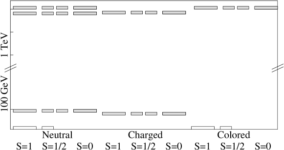
Figure 1: The particle spectrum with unbroken SUSY for a typical set of parameters $Rk\pi\simeq$ $37.5$ ($k\simeq\Lambda_{\text{Pl}}$). The $S=1/2$ bars each represent one Majorana particle in the neutral column and one Dirac particle in the charged column, while the filled/unfilled $S=1$ bars distinguish between massive/massless vectors with three/two physical degrees of freedom

Of course, similarly to the MSSM, such a spectrum is not acceptable because massless neutralinos, gluinos and light charginos below 95 GeV have already been ruled out by experimental searches. Also, the gauge scalars are even under $R$ parity and could be produced below the pair production threshold. We will therefore investigate the consequences of having no supersymmetry at all on the UV brane. Starting from this premise, it is natural to remove all scalars from the UV brane by imposing the BCs

$$\Sigma^{L}(0)=\Sigma^{R}(0)=\Sigma^{X}(0)=\Sigma^{C}(0)=h_{L}^{i}(0)=h_{R}^{ic}(0)=0\,.$$ (21)

This pushes the $SU(3)$ and $U(1)_{X}$ gauge scalars up to a mass

$$m_{\Sigma^{C}}=m_{\Sigma^{X}}=z_{0}k\mathrm{e}^{-Rk\pi}\simeq z_{0}\sqrt{Rk\pi(1+\kappa)}\,m_{W}\simeq 1.2\,\mathrm{TeV}$$ (22)

where $z_{0}\simeq 2.41$ is the first zero of the Bessel function $J_{0}(z)$. The sfermions lie in a similar mass range, depending on the localization parameter $c$ of the multiplet. For a massless fermion we can approximate the tree level sfermion masses

$$m_{\tilde{f}} =z_{0}k\mathrm{e}^{-Rk\pi}\,,$$ (23)

where, if $c_{L}\neq 1/2,c_{R}\neq-1/2$, $z_{0}$ is the first positive root of $J_{c_{L}-1/2}$ for $\tilde{f}_{L}$, $J_{|c_{R}+1/2|}$ for $\tilde{f}_{R}$, $J_{|c_{L}-1/2|}$ for $\tilde{f}_{L}^{c}$ and $J_{-c_{R}-1/2}$ for $\tilde{f}_{R}^{c}$. The situation is different for the scalars from gauge groups that are broken on the IR brane. These scalars receive smaller tree level masses

$$m_{\Sigma^{0}}=m_{\Sigma^{+}}\simeq\sqrt{\frac{2k}{R\pi}}\mathrm{e}^{-Rk\pi}=\sqrt{2(1+\kappa)}\,m_{W}\,,$$ (24)

which is very interesting from a phenomenological point of view. However, their tree level coupling to fermions is of the form $\Sigma\psi\psi^{c}$ and therefore suppressed with the fermion mass, vanishing altogether in the massless fermion limit where it is forbidden by the chiral symmetry. For a large range of parameters, the coupling to leptons and quarks is similar to the corresponding SM Higgs coupling. Note however that since it is not the vacuum expectation value of this scalar triplet that breaks electroweak symmetry, this similarity does not extend to the coupling to gauge bosons. Consequently, the processes corresponding to Higgsstrahlung and vector boson fusion in the SM are absent in our model at tree level. This provides an experimental signature for distinguishing our model from the MSSM at the upcoming LHC experiments.

Now let us turn to the gauginos. We split the gauginos and the gauge bosons with the localized kinetic term (57). We will study the following two sets of BCs which project out all massless modes, while maintaining the $SU(2)_{L}\times U(1)_{Y}$ invariance (but not the full supergauge invariance) and the stationarity of the action on the UV brane. In the first scenario

$$\lambda_{2}^{L}=\lambda_{1}^{R}=\lambda_{1}^{X}=0\,,$$ (25a)

while in the second

$$\lambda^{L}_{1} =\lambda^{R12}_{2}=0$$ (25b)

$$\cos(\theta)\lambda^{X}_{1}+\sin(\theta)\lambda^{R3}_{1} =\cos(\theta)\lambda^{R3}_{2}-\sin(\theta)\lambda^{X}_{2}=0\,.$$

In both cases, the lightest charginos will receive a tree level mass

$$m_{\chi^{+}}\simeq\sqrt{1+\kappa}\,m_{W}\,,$$ (26)

which requires $\kappa\geq 0.4$ to escape the current detection bounds. The resulting mass of the lightest neutralino mode will then be

$$m_{\chi^{0}}=m_{\chi^{+}}$$ (27a)

in the first scenario (25a) and

$$m_{\chi^{0}}\simeq\cos(\theta)\,m_{\chi^{+}}$$ (27b)

in the second (25b).

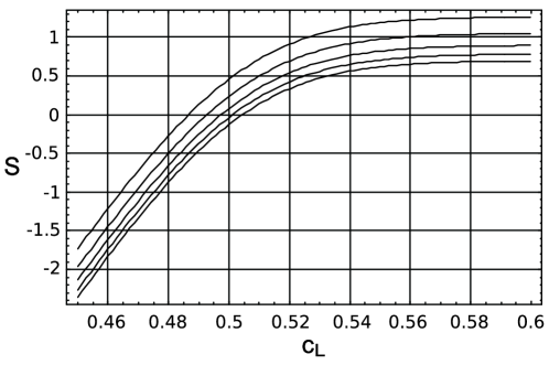
Figure 2: The tree level contribution to the S parameter for a massless probe fermion, $Rk\pi\simeq 37.5$, $k\simeq\Lambda_{\text{Pl}}$ , $c_{R}=-c_{L}$ and different values of $\kappa$. ($\kappa=0,0.2,0.4,0.6,0.8$ from highest to lowest)

If we isolate the oblique corrections that arise at tree level analogous to [21, 7], there are two parameters that have a strong influence on the parameters $S$, $T$ and $U$ in our scenarios, namely $\kappa$ and the fermion localization parameters $c$. Using the method of these authors, the resulting value for $S$ is given in fig. 2. We find a combination of the results in [7] and [21]. The kinetic term used to split the electroweak gauge multiplets moves $S$ in the right direction and can allow for delocalized or slightly UV localized fermions.

3.3 Supergravity

In some supersymmetric extensions of the SM, the gravitino poses a problem for cosmological observables, either because it is overabundant or so long-lived that its decay products spoil nucleosynthesis. So far we have not included supergravity in the bulk, and we want to give an argument that the inclusion of KK gravitons and gravitinos in the bulk is possible without loosing the desired properties of the model. A holographic interpretation along the AdS/CFT correspondence where the energy momentum tensor and the supersymmetric currents are present on the CFT side also warrants the inclusion of supersymmetric gravity multiplets. Similarly to BC gauge symmetry breaking we adopt the philosophy that the simple picture with BCs is a description mimicking a full theory with symmetry breaking in a slice of AdS5 [15, 22]. By setting the appropriate BCs we obtain a heavy short-lived gravitino.

Solving and KK expanding the (free) Rarita-Schwinger equations with “twisted” IR BCs $\psi_{2}^{\mu}(0)=\psi_{1}^{\mu}(\pi)=0$, we obtain a very light gravitino $m_{0}\simeq\sqrt{8}k\mathrm{e}^{-2Rk\pi}$[20]. However, twisting the BC on the UV brane yields the condition

$$\frac{J_{2}(\frac{m}{k})}{Y_{2}(\frac{m}{k})}-\frac{J_{1}(\mathrm{e}^{Rk\pi}\frac{m}{k})}{Y_{1}(\mathrm{e}^{Rk\pi}\frac{m}{k})}=0\quad\longrightarrow\quad m_{n}\simeq z_{n}k\mathrm{e}^{-Rk\pi}\,,$$

where $z_{n}$ are the positive roots of $J_{1}$. From $z_{0}\approx 3.83$ we find a heavy gravitino solution at the scale of the lightest graviton KK mode ($\mathcal{O}(2\,\mathrm{TeV})$ for $k=\Lambda_{\text{Pl}}$). Like the heavy gravitons, this gravitino does not have Planck suppressed interactions but rather a coupling $\lesssim\mathrm{TeV}^{-1}$ depending on the localization parameters. To be more precise, let us calculate the coupling scales relevant for neutralino annihilation (and gravitino decay). The general solutions for the KK wave functions are (cf., e. g., [20, 22, 23])

$$\tilde{G}^{(n)}_{1}(y) =\mathrm{e}^{2Rky}\left[\alpha\,J_{2}(m_{n}\,\mathrm{e}^{Rky}/k)+\beta\,Y_{2}(m_{n}\,\mathrm{e}^{Rky}/k)\right]$$ (28)

$$\tilde{G}^{(n)}_{2}(y) =\mathrm{e}^{2Rky}\left[\alpha\,J_{1}(m_{n}\,\mathrm{e}^{Rky}/k)+\beta\,Y_{1}(m_{n}\,\mathrm{e}^{Rky}/k)\right]=\frac{\mathrm{e}^{-Rky}}{R\,m_{n}}\partial_{y}\tilde{G}^{(n)}_{1}\,,$$ (29)

with the canonical normalization condition

$$\int\!\mathrm{d}y\,\mathrm{e}^{-2Rky}G^{2}_{i}(y)=1\,.$$

With these conventions, the coupling strength to a vector and a gaugino is

$$\langle\tilde{G}_{i}f_{V}f_{\chi_{i}}\rangle =\frac{1}{\Lambda_{\text{Pl}}}\sqrt{\frac{R}{2k}}\int\!\mathrm{d}y\mathrm{e}^{-3/2Rky}\,\tilde{G}_{i}f_{V}f_{\chi_{i}}\,.$$ (30)

The normalization is chosen such that a gravitino zero mode with unbroken SUSY would yield $\langle\tilde{G}_{1}^{(0)}f_{V}f_{\chi_{1}}\rangle=\Lambda_{\text{Pl}}^{-1}$, $\tilde{G}_{2}^{(0)}=0$. For $\kappa=0.4$ and $k=\Lambda_{\text{Pl}}$ we obtained

$$\langle\tilde{G}_{1}f_{Z}f_{\chi^{0}_{1}}^{(1)}\rangle \approx(500\,\mathrm{TeV})^{-1} \langle\tilde{G}_{2}f_{Z}f_{\chi^{0}_{2}}^{(1)}\rangle \approx(25\,\mathrm{TeV})^{-1}$$ (31a)

$$\langle\tilde{G}_{1}f_{Z}^{(2)}f_{\chi^{0}_{1}}^{(1)}\rangle \approx(10\,\mathrm{TeV})^{-1} \langle\tilde{G}_{2}f_{Z}^{(2)}f_{\chi^{0}_{2}}^{(1)}\rangle \approx(80\,\mathrm{TeV})^{-1}$$ (31b)

$$\langle\tilde{G}_{1}f_{Z}^{(2)}f^{(2)}_{\chi^{0}_{1}}\rangle \approx(1\,\mathrm{TeV})^{-1} \langle\tilde{G}_{2}f_{Z}^{(2)}f^{(2)}_{\chi^{0}_{2}}\rangle \approx(3\,\mathrm{TeV})^{-1}\,.$$ (31c)

Considering the usual holographic picture, this result is not surprising, because the heavy gravitino is interpreted as a bound state with TeV suppressed interactions to other bound states (31c), coupling less strongly to lighter, mostly elementary particles (31a) and (31b). With the result in (31a) for the SM couplings we can neglect neutralino annihilation with the gravitino in the $t$-channel in the following discussion. Still, such a gravitino couples strongly enough to essentially vanish immediately for a temperature of $T\ll 2\,\mathrm{TeV}$, long before nucleosynthesis.

4 Dark Matter Phenomenology

Our aim in this section is to estimate the relic density of the neutralino LSP we found in the scenarios discussed above. The analysis of thermal WIMP production and relic densities generally requires to numerically solve the Boltzmann equation for the scattering processes involved, but there are approximate semi-analytic solutions adequate for WIMPs in SM extensions. In our calculation of the neutralino freezeout temperature and relic density we follow [11, 10]. In the case without coannihilations we need the number of effectively massless degrees of freedom $g^{*}$, the LSP mass and the total cross section $\chi_{i}^{0}\chi_{j}^{0}\rightarrow X$ expanded in the relative velocity $v$

$$v\sigma^{tot}_{ij}(v)=a_{ij}+b_{ij}\,v+\mathcal{O}(v^{2})\,,$$ (32)

which we obtain by evaluating the graphs in Fig. 3. The cross section (32) can be reexpressed in terms of the temperature $T$

$$\langle v\sigma^{tot}_{ij}\rangle(T)\simeq a_{ij}+b_{ij}\,\frac{6\,T}{m_{\chi^{0}}}\,.$$ (33)

The relative freezeout temperature $1/x_{f}=T_{f}/m_{\chi^{0}}$ can be determined iteratively, and is typically at around $x_{f}\approx 15\dots 25$. The final expression for the relic density is then

$$\Omega h^{2}(x_{f})=\frac{1.04\times 10^{9}\,\mathrm{GeV}^{-1}}{\Lambda_{\text{Pl}}}\frac{x_{f}}{\sqrt{g^{*}}}\frac{1}{a+3b/x_{f}}\,.$$ (34)

The effective number of degrees of freedom is taken to be $g^{*}=86\frac{1}{4}$, to which fermions contribute with a weight of $7/8$ from the Fermi distribution. To give an estimate of the individual contributions $\chi_{i}^{0}\chi_{j}^{0}\rightarrow X_{n}$, we will add the inverse densities

$$1/\Omega h^{2}(x_{f})=\sum_{n}{\Omega h^{2}_{n}}(x_{f})^{-1}\propto\sum_{n}a_{n}\!+3\,b_{n}/x_{f}$$ (35)

for a realistic fixed freezeout temperature, which depends only weakly on the cross section. The value currently favored by WMAP data is $1/{\Omega h^{2}}\approx 9\dots 11$ [9].

4.1 Neutralino Annihilation Channels

Figure 3: Tree level contributions to neutralino annihilation.

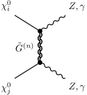
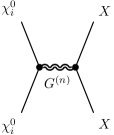
Figure 4: Potential tree level contributions to neutralino annihilation from the gravitinos and massive gravitons

Depending on the neutralino mass there are several annihilation channels contributing at tree level (Fig. 3). The channels $\chi_{i}^{0}\chi_{j}^{0}\rightarrow l\overline{l},\nu\overline{\nu}$ and $\chi_{i}^{0}\chi_{j}^{0}\rightarrow d\overline{d},u\overline{u},s\overline{s},c\overline{c},b\overline{b}\to\text{jets}$ are always open, whereas $\chi_{i}^{0}\chi_{j}^{0}\rightarrow W^{+}W^{-}$ is open for all parameters in scenario (25a) but only if $\cos{\theta}\sqrt{1+\kappa}>1$ in scenario (25b). We first rewrite the neutralinos (charginos) as two Majorana (Dirac) fermions. To achieve this, we express the 4D action in terms of the KK coefficient fields $\lambda_{1}^{1,2(n)}(x)$, $\lambda_{2}^{1,2(n)}(x)$, $\lambda_{1}^{0(n)}(x)$ and $\lambda_{2}^{0(n)}(x)$ and group those into 4 spinors (the KK indices are implicit)

$$\chi^{0}_{a}(x) =\frac{1}{\sqrt{2}}\left(\lambda_{1}^{0}+\lambda_{2}^{0},\overline{\lambda_{1}^{0}}+\overline{\lambda_{2}^{0}}\right)$$

$$\chi^{0}_{b}(x) =\frac{i}{\sqrt{2}}\left(\lambda_{1}^{0}-\lambda_{2}^{0},\overline{\lambda_{2}^{0}}-\overline{\lambda_{1}^{0}}\right)$$

$$\chi^{+}_{a}(x) =\frac{1}{\sqrt{2}}\left(\lambda_{1}^{1}-i\lambda_{1}^{2},\overline{\lambda_{2}^{1}}-i\overline{\lambda_{2}^{2}}\right)$$

$$\chi^{+}_{b}(x) =\frac{1}{\sqrt{2}}\left(\lambda_{2}^{1}-i\lambda_{2}^{2},\overline{\lambda_{1}^{1}}-i\overline{\lambda_{1}^{2}}\right)$$

With these definitions, the full 4D chargino-matter-smatter interaction Lagrangian takes the form

$$\mathcal{L} =h_{j}\,\overline{\Psi}_{i}i\Gamma_{ij}(\chi_{a}^{0}+i\chi_{b}^{0})+h_{j}^{c\dagger}\,\overline{\Psi}_{i}i\Gamma^{c}_{ij}(\chi_{a}^{0}-i\chi_{b}^{0})+\text{h.c.}\,.$$ (36)

The vertices are given in terms of the projectors, overlap integrals and quantum numbers by

$$\Gamma_{ij} =g_{5}T_{ij}^{3L}\left[P^{-}\langle f_{\lambda_{1}^{L3}}f_{\psi_{Li}}f_{h_{Lj}}\rangle-P^{+}\langle f_{\lambda_{2}^{L3}}f_{\psi_{Li}^{c}}f_{h_{Lj}}\rangle\right]$$

$$+g_{5}T_{ij}^{3R}\!\left[P^{-}\langle f_{\lambda_{1}^{R3}}f_{\psi_{Ri}}f_{h_{Rj}}\rangle-P^{+}\langle f_{\lambda_{2}^{R3}}f_{\psi_{Ri}^{c}}f_{h_{Rj}}\rangle\right]$$

$$+\tilde{g}_{5}X_{ij}\left[P^{-}\langle f_{\lambda_{1}^{X}}f_{\psi_{Li}}f_{h_{Lj}}\rangle-P^{+}\langle f_{\lambda_{2}^{X}}f_{\psi_{Li}^{c}}f_{h_{Lj}}\rangle\right]$$

$$+\tilde{g}_{5}X_{ij}\left[P^{-}\langle f_{\lambda_{1}^{X}}f_{\psi_{Ri}}f_{h_{Rj}}\rangle-P^{+}\langle f_{\lambda_{2}^{X}}f_{\psi_{Ri}^{c}}f_{h_{Rj}}\rangle\right]$$

$$\Gamma_{ij}^{c} =g_{5}T_{ij}^{3L}\left[P^{-}\langle f_{\lambda_{2}^{L3}}f_{\psi_{Li}}f_{h_{Lj}^{c}}\rangle+P^{+}\langle f_{\lambda_{1}^{L3}}f_{\psi_{Li}^{c}}f_{h_{Lj}^{c}}\rangle\right]$$

$$+g_{5}T_{ij}^{3R}\left[P^{-}\langle f_{\lambda_{2}^{R3}}f_{\psi_{Ri}}f_{h_{Rj}^{c}}\rangle+P^{+}\langle f_{\lambda_{1}^{R3}}f_{\psi_{Ri}^{c}}f_{h_{Rj}^{c}}\rangle\right]$$

$$+\tilde{g}_{5}X_{ij}\left[P^{-}\langle f_{\lambda_{2}^{X}}f_{\psi_{Li}}f_{h_{Lj}^{c}}\rangle+P^{+}\langle f_{\lambda_{1}^{X}}f_{\psi_{Li}^{c}}f_{h_{Lj}^{c}}\rangle\right]$$

$$+\tilde{g}_{5}X_{ij}\left[P^{-}\langle f_{\lambda_{2}^{X}}f_{\psi_{Ri}}f_{h_{Rj}^{c}}\rangle+P^{+}\langle f_{\lambda_{1}^{X}}f_{\psi_{Ri}^{c}}f_{h_{Rj}^{c}}\rangle\right]\,.$$

In this expression, the brackets $\langle f_{\lambda}f_{\psi}f_{h}\rangle\equiv\int\!\mathrm{d}y\sqrt{g}\,f_{\lambda}(y)f_{\psi}(y)f_{h}(y)$ stand for the 5D overlaps which give us the coupling strengths of a sfermion to the corresponding matter fermion and a neutralino. The structure is such that the “left handed” sfermion couples to gauginos and matter fermions of the same handedness, the “right handed” one to gauginos and matter fermions of opposite handedness. The charged current interaction Lagrangian is

$$\mathcal{L}=-\frac{1}{\sqrt{2}}W_{m}^{+}\left[\overline{\chi^{+}_{a}}\,\Gamma^{m}_{a}\left(\chi^{0}_{a}-i\chi^{0}_{b}\right)+\overline{\chi^{+}_{b}}\,\Gamma^{m}_{b}\left(\chi^{0}_{a}+i\chi^{0}_{b}\right)\right]+\text{h.c.}$$ (37)

and the corresponding vertex expressions are

$$\Gamma_{a}^{n} =g_{5}\gamma^{n}\left[P^{-}(\langle f_{W^{L\pm}}f_{\lambda^{L\pm}_{2}}f_{\lambda^{L3}_{2}}\rangle+\langle f_{W^{R\pm}}f_{\lambda^{R\pm}_{2}}f_{\lambda^{R3}_{2}}\rangle)\right.$$

$$\left.\hskip 17.22217pt+P^{+}(\langle f_{W^{L\pm}}f_{\lambda^{L\pm}_{1}}f_{\lambda^{L3}_{1}}\rangle+\langle f_{W^{R\pm}}f_{\lambda^{R\pm}_{1}}f_{\lambda^{R3}_{1}}\rangle)\right]$$

$$\Gamma_{b}^{n} =\Gamma_{a}^{n}(P^{+}\leftrightarrow P^{-})\,,$$

with the 5D overlap integrals $\langle f_{W}f_{\lambda_{i}}f_{\lambda_{j}}\rangle\equiv\int\!\mathrm{d}y\sqrt{g}\,\mathrm{e}^{Rky}f_{W}(y)f_{\lambda_{i}}(y)f_{\lambda_{j}}(y)$ which now have an additional factor $\mathrm{e}^{Rky}$ from the inverse vielbein contained in $\gamma^{\mu}$. The effective coupling constants for the charged current can be approximated analytically to leading order using $Rk\pi\gg 1$ and $m_{W},m_{\chi}\ll k\mathrm{e}^{-Rk\pi}$ as

$$\langle f_{W^{L\pm}}f_{\lambda^{L\pm}_{2}}f_{\lambda^{L3}_{2}}\rangle\simeq-\frac{3}{8}C\qquad\langle f_{W^{R\pm}}f_{\lambda^{R\pm}_{2}}f_{\lambda^{R3}_{2}}\rangle\simeq-\frac{1}{8}C\,,$$ (38)

with

$$\langle f_{W^{L\pm}}f_{\lambda^{L\pm}_{1}}f_{\lambda^{L3}_{1}}\rangle\simeq-C\qquad\langle f_{W^{R\pm}}f_{\lambda^{R\pm}_{1}}f_{\lambda^{R3}_{1}}\rangle\simeq-\frac{1}{48Rk\pi}C$$ (39a)

in scenario (25a) and

$$\langle f_{W^{L\pm}}f_{\lambda^{L\pm}_{1}}f_{\lambda^{L3}_{1}}\rangle\simeq-\frac{|\cos(\theta)|}{24Rk\pi}C\qquad\langle f_{W^{R\pm}}f_{\lambda^{R\pm}_{1}}f_{\lambda^{R3}_{1}}\rangle\simeq-\frac{7|\cos(\theta)|}{48Rk\pi}C$$ (39b)

in scenario (25b), respectively, where

$$C=\frac{1}{\sqrt{(\kappa+1)R\pi}}\,.$$ (40)

They are accurate to about $5\%$ for $Rk\pi>30$ (cf. also Fig. 5 below). Note that the absolute size of the coupling is approximately independent of the free parameters,

$$g_{5}C\simeq\frac{\sqrt{4\pi\alpha}}{\sin(\theta_{W})}\,,$$ (41)

and the leading contributions are also independent of the neutralino mass. For the sfermions with $m_{\widetilde{f}}>k\mathrm{e}^{-Rk\pi}$ the same expansion is not possible. The Feynman rules were implemented and the cross sections evaluated using FeynArts/FormCalc [24].

4.2 Results

4.2.1 Annihilation into Fermions

Due to the large KK mass of the sfermions around $-c_{R},c_{L}\approx 0.2\dots 0.7$ of $m_{\widetilde{f}}>2k\mathrm{e}^{-Rk\pi}$, the cross sections $\chi^{0}\chi^{0}\rightarrow\overline{f}f$ will be suppressed relative to the annihilation to $W$ pairs if $m_{\chi^{0}}>m_{W}$. We find that the couplings and cross section depend strongly on the localization of the fermion multiplets, but that a rather extreme localization towards the TEV brane is necessary to make a significant contribution to the total annihilation cross section. This region of parameter space is ruled out due to FCNCs (unless an additional flavor symmetry is introduced to suppress them) and proton decay from higher dimensional operators. Therefore we conclude that in this scenario the tree level annihilation of neutralinos into fermions is negligible. For example, if one carries out the calculation for $k=\Lambda_{\text{Pl}}$, $\kappa=.4$, $x_{f}=23$ the contribution of the charm quark stays below $1/\Omega h^{2}<0.3$ for $|c_{L,R}|>0.25$ and even $1/\Omega h^{2}<0.02$ for $|c_{L,R}|>0.5$. The electron which must be at $c_{L}\approx 0.5$ to get a realistic $S$ parameter, contributes $1/\Omega h^{2}<0.01$. One uncertainty comes from the precise implementation of the third quark generation. The straightforward generation of $m_{b}$ and $m_{t}$ with boundary terms leads to problems with the $Zb\overline{b}$ coupling. Depending on how the $b$ quark is realized, its coupling to the neutralino could be somewhat enhanced, but we can still expect that the channel $\chi^{0}_{i}\chi^{0}_{j}\rightarrow b\overline{b}$ does not play a major role for dark matter annihilation.

4.2.2 Annihilation into $W$ Pairs

If $m_{\chi^{0}}>m_{W}$, the neutralino LSP can annihilate into two $W$s at tree level, and the interaction is essentially of weak strength (41). In scenario (25a) the annihilation cross section turns out to be too large, leading to a small relic density which would require another mechanism for Dark Matter production. In scenario (25b) the largest coupling constants are strongly suppressed, and the relic density is in a realistic range (Fig. 5). A neutralino LSP with $m_{\chi^{0}}\gtrsim 86\,\mathrm{GeV}$ is favored.

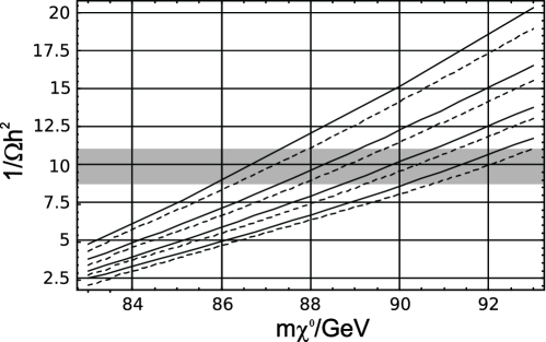
Figure 5: The $m_{\chi^{0}}$-dependence of contributions to $1/\Omega h^{2}$ for annihilation into $W$ pairs for $Rk\pi\simeq 37.5$, $k=\Lambda_{\text{Pl}}$. The parameter is (from topmost) $\kappa=0.4,0.6,0.8,1.0$, corresponding to $m_{\chi^{+}}=95,102,108,114$ GeV. For this process we use $\alpha=1/128$. The dashed lines are obtained using the approximations in (38)-(41). The shaded area represents the region allowed by the WMAP three year data.

5 Conclusions

We have constructed a minimal supersymmetric extension of warped higgsless models. The absence of SUSY on the UV brane leads to a tree level spectrum in which the lightest neutralinos are naturally the lightest superpartners and the lightest charginos the NLSPs. Experimental constraints force us to shift the chargino mass above $95\,\mathrm{GeV}$, with $m_{\chi^{0}}=0\,\ldots\,m_{\chi^{+}}$ depending on the mixing angle. All color charged superpartners and the sfermions are at the KK scale $\lesssim\mathcal{O}(\mathrm{TeV})$.

The lightest electroweak gauge scalars $\Sigma^{\pm}$, $\Sigma^{0}$ have tree level masses at $\sqrt{2}\,m_{\chi^{+}}$, but are expected to receive significant radiative corrections. Their Higgs-like masses and couplings to matter make them an interesting object for searches at the LHC, where they could be distinguished from the Higgs by the absence of Higgsstrahlung and vector boson fusion processes. These issues will be treated in an upcoming publication, along with a more detailed analysis of LEP precision observables.

Another aspect to be investigated is tree level unitarity of the model which generally requires vector boson KK modes lighter than the ones found in our minimal scenario, a feature which can for example be achieved by including additional boundary terms.

For $m_{\chi^{0}}>m_{W}$, the dominant channel for LSP annihilation is into $W$ pairs, while the annihilation into SM fermions does not contribute significantly unless they are highly localized towards the TeV brane. If the left-handed neutralino is set up to be localized mostly in the $SU(2)_{R}$ triplet, the LSP relic density is in agreement with current observations for a natural range of parameters where $m_{W}<m_{\chi^{0}}<m_{\chi^{+}}$, making SUSY in the EWSB sector a promising source for the observed nonbaryonic dark matter if Higgsless symmetry breaking turns out to be realized in nature.

Appendix A Conventions

We use the flat metric convention $\eta=\text{diag}(+,-,-,-,-)$ and the corresponding Dirac matrices

$$\gamma^{m}=-\left(\begin{array}[]{cc}0&\sigma^{m}\\ \overline{\sigma}^{m}&0\end{array}\right)~{}~{}\gamma^{\bar{5}}=\left(\begin{array}[]{cc}i&0\\ 0&-i\end{array}\right)\,,$$ (46)

where $\sigma^{0}=\overline{\sigma}^{0}=-1$ and $-\overline{\sigma}^{i}=\sigma^{i}$ are the Pauli matrices. We define the projectors

$$P^{+}=\frac{1}{2}(-i\gamma^{\bar{5}}+1)\quad P^{-}=\frac{1}{2}(-i\gamma^{\bar{5}}-1)$$ (47)

on the 4D “left handed” and “right handed” component respectively. For Dirac spinors $\Psi^{T}=(\eta_{\alpha},\overline{\chi}^{\dot{\alpha}})$ we define $\overline{\Psi}=\Psi^{\dagger}\gamma^{\overline{0}}=(\chi^{\alpha},\overline{\eta}_{\dot{\alpha}})$.

Two coordinate systems are commonly used. The “proper distance” coordinates have $x^{M}=(x^{\mu},y)$ and $y\in[0,\pi]$. They are related to the “conformal” coordinates with $x^{M}=(x^{\mu},z)$, $z\in[k^{-1},\Lambda_{\text{IR}}^{-1}]$ through

$$z=k^{-1}\mathrm{e}^{Rky}\qquad\Lambda_{\text{IR}}=k\mathrm{e}^{-Rk\pi}\,.$$ (48)

The Dirac matrices read in proper distance coordinates

$$\gamma^{\mu} =-\delta^{\mu}_{m}\mathrm{e}^{Rky}\left(\begin{array}[]{cc}0&\sigma^{m}\\ \overline{\sigma}^{m}&0\end{array}\right)$$ (49c)

$$\gamma^{5} =\frac{1}{R}\left(\begin{array}[]{cc}i&0\\ 0&-i\end{array}\right)$$ (49f)

$$\gamma_{\mu} =\eta_{\mu\nu}\mathrm{e}^{-2Rky}\gamma^{\nu}$$ (49g)

$$\gamma_{5} =-R^{2}\gamma^{5}$$ (49h)

and in conformal coordinates

$$\gamma^{\mu} =-\delta^{\mu}_{m}kz\left(\begin{array}[]{cc}0&\sigma^{m}\\ \overline{\sigma}^{m}&0\end{array}\right)$$ (50c)

$$\gamma^{5} =kz\left(\begin{array}[]{cc}i&0\\ 0&-i\end{array}\right)$$ (50f)

$$\gamma_{\mu} =\eta_{\mu\nu}\frac{1}{k^{2}z^{2}}\gamma^{\nu}$$ (50g)

$$\gamma_{5} =-\frac{1}{k^{2}z^{2}}\gamma^{5}\,.$$ (50h)

Appendix B Boundary Conditions and KK Decomposition

Boundary Conditions

The kinetic terms that we obtain straight from the superfield action and the BCs take the canonical form after the field redefinitions

$$\psi\longrightarrow\mathrm{e}^{-\frac{1}{2}Rky}\psi A_{\mu}\longrightarrow gA_{\mu} \lambda_{1}\longrightarrow g\mathrm{e}^{-\frac{3}{2}Rky}\lambda_{1}$$ (51)

$$A_{5}\longrightarrow gRA_{5} \lambda_{2}\longrightarrow-igR\mathrm{e}^{-\frac{1}{2}Rky}\lambda_{2} \Sigma\longrightarrow gR\Sigma$$

The standard coupling constants are recovered after taking $g_{5}\equiv g/2$. Before we specify the KK decomposition for the fields, we employ an $R_{\xi}$ type gauge fixing term

$$S_{gf}=-\int\!\mathrm{d}^{5}x\,\frac{R}{2\xi}\left(\eta^{mn}\partial_{m}A_{n}-\xi\frac{\mathrm{e}^{-2Rky}}{R}(\partial_{y}-2Rk)A_{5}\right)^{2}\,.$$ (52)

The BCs in (20) now give the KK modes $A_{5}^{(n)}$ an unphysical mass $\sqrt{\xi}m_{n}$ if the corresponding massive gauge boson mode has a mass $m_{n}$. This can be seen as follows: With (52) and (10) the KK equations of motion are

$$m_{n}^{2}A^{(n)}_{\mu} =\mathrm{e}^{-2Rky}(-\partial_{y}^{2}/R^{2}+2k\partial_{y}/R)A^{(n)}_{\mu}$$

$$m_{n}^{2}A^{(n)}_{5} =\mathrm{e}^{-2Rky}(-\partial_{y}^{2}/R^{2}+4k\partial_{y}/R-4k^{2})A_{5}^{(n)}\,.$$

Taking the derivative of the first equation, we find

$$m_{n}^{2}\partial_{y}A^{(n)}_{\mu} =\mathrm{e}^{-2Rky}(-\partial_{y}^{2}/R^{2}+4k\partial_{y}/R-4k^{2})\partial_{y}A^{(n)}_{\mu}\,.$$ (53)

Since $\partial_{y}A_{\mu}$ satisfies the same equation of motion as $A_{5}$, the correct choice of BCs immediately follows:

$$\partial_{y}A_{\mu}|_{\partial}=0 \Longrightarrow A_{5}|_{\partial}=0$$ (54)

$$A_{\mu}|_{\partial}=0 \stackrel{{\scriptstyle m_{n}\neq 0}}{{\Longrightarrow}}(\partial_{y}-2Rk)A_{5}|_{\partial}=0\,.$$

Now, there is a mode of $A_{5}$ for every massive mode of $A_{\mu}$. A similar reasoning applies to the fermions. Consider the action for any gaugino,

$$\int\!\mathrm{d}^{5}x\>R\mathrm{e}^{-3Rky}(-i\lambda_{i}\sigma^{n}\partial_{n}\overline{\lambda}_{i})+\int\!\mathrm{d}^{5}x\>R\mathrm{e}^{-4Rky}\left[-\lambda_{2}\frac{\partial_{y}-3/2Rk}{R}\lambda_{1}+c.c.\right]\,.$$ (55)

The KK decomposition for these coupled differential equations diagonalizes the KK Dirac mass if

$$(\partial_{y}-3/2Rk)\lambda_{1}=0 \Rightarrow\lambda_{2}=0$$ (56)

$$\lambda_{1}=0 \Rightarrow(\partial_{y}-5/2Rk)\lambda_{2}=0$$

This choice is again related to (53) by (7).

Brane Kinetic Terms

We will eventually introduce a gauge invariant UV brane kinetic term for the $SU(2)_{L}$ gauge bosons to split the $W^{\pm}$ and the charginos. Localized gauge kinetic terms modify the BCs, the definition of the scalar product and of the coupling constants. For example, such a term for the $SU(2)_{L}$ vectors

$$S\rightarrow S+\kappa\int\!\mathrm{d}^{5}x\,\delta(y)\pi R\,\left(-\frac{1}{4}\eta^{mo}\eta^{np}L^{a}_{mn}L^{a}_{op}\right)\,,$$ (57)

leads to the canonical normalization conditions for the $W^{\pm}$, $Z$ and photon

$$\int\!\!\mathrm{d}y\,R\Big{(}f^{L12(n)}(y)^{2}+f^{R12(n)}(y)^{2}\Big{)}+\pi R\kappa f^{L12(n)}(0)^{2}=1$$ (58)

$$\int\!\!\mathrm{d}y\,R\Big{(}f^{L3(n)}(y)^{2}+f^{R3(n)}(y)^{2}+f^{X(n)}(y)^{2}\Big{)}+\pi R\kappa f^{L3(n)}(0)^{2}=1$$ (59)

$$\pi R\left((2+\kappa)\left(\frac{a_{0}}{g_{5}}\right)^{2}+\left(\frac{a_{0}}{\tilde{g}_{5}}\right)^{2}\right)=1\,.$$ (60)

The Neumann BC $\partial_{y}A^{L}_{\mu}(0)=0$ becomes

$$\left(\partial_{y}+m^{2}\pi R^{2}\kappa\right)A^{L}_{\mu}(0)=0\,.$$

The dimensionless constant $\kappa$ is naturally $\simeq\mathcal{O}(1)$.

KK Decomposition

The 5D fields are split into a coefficient bearing the 4D dependence, and the KK wavefunctions

$$\phi(x,y)=\sum_{n}\phi^{(n)}(x)f^{(n)}(y)\,.$$ (61)

The canonical normalization of the wavefunctions is $\int_{0}^{\pi}\!\mathrm{d}y\,Rf(y)^{2}=1$ in flat space, but depends on the field in warped space because of the factor $\sqrt{g}$ and the different number of vielbeins $e_{\mu}^{n}$. For vectors, spinors and scalars respectively it is

$$\int\!\!\mathrm{d}yRf_{V}^{2}(y)=1,\quad\int\!\!\mathrm{d}yR\mathrm{e}^{-3Rky}f_{\Psi}^{2}(y)=1,\quad\int\!\!\mathrm{d}yR\mathrm{e}^{-2Rky}f_{\Sigma}^{2}(y)=1\,.$$ (62)

Any BC mixing two fields on the boundaries causes the two fields to belong to the same 4D KK tower, e.g. $A_{\mu}^{L(n)}\!(x)f^{L(n)}(y)=A_{\mu}^{R(n)}\!(x)f^{R(n)}(y)$ requires $A_{\mu}^{L(n)}(x)=A_{\mu}^{R(n)}(x)$ to have the free action diagonal in the KK modes. Canonical normalization then means that the sum of the normalizations of all fields coupled in this manner should be unity.

References

- [1] S. Weinberg, Phys. Rev. D13, 974 (1976).
- [2] N. D. Christensen and R. Shrock, Phys. Lett. B632, 92 (2006), [arXiv:hep-ph/0509109].
- [3] N. D. Christensen and R. Shrock, Phys. Rev. D74, 015004 (2006), [arXiv:hep-ph/0603149].
- [4] C. Csaki, C. Grojean, H. Murayama, L. Pilo, and J. Terning, Phys. Rev. D69, 055006 (2004), [arXiv:hep-ph/0305237].
- [5] C. Csaki, C. Grojean, L. Pilo, and J. Terning, Phys. Rev. Lett. 92, 101802 (2004), [arXiv:hep-ph/0308038].
- [6] H. Davoudiasl, J. L. Hewett, B. Lillie, and T. G. Rizzo, JHEP 05, 015 (2004), [arXiv:hep-ph/0403300].
- [7] G. Cacciapaglia, C. Csaki, C. Grojean, and J. Terning, Phys. Rev. D71, 035015 (2005), [arXiv:hep-ph/0409126].
- [8] G. Cacciapaglia, C. Csaki, G. Marandella, and J. Terning, Phys. Rev. D75, 015003 (2007), [arXiv:hep-ph/0607146].
- [9] WMAP, D. N. Spergel et al., Astrophys. J. Suppl. 170, 377 (2007), [arXiv:astro-ph/0603449].
- [10] G. Servant and T. M. P. Tait, Nucl. Phys. B650, 391 (2003), [arXiv:hep-ph/0206071].
- [11] K. Kong and K. T. Matchev, JHEP 01, 038 (2006), [arXiv:hep-ph/0509119].
- [12] K. Agashe, A. Falkowski, I. Low, and G. Servant, [arXiv:0712.2455 [hep-ph]].
- [13] G. Panico, E. Ponton, J. Santiago, and M. Serone, [arXiv:0801.1645 [hep-ph]].
- [14] M. F. Sohnius, Phys. Rept. 128, 39 (1985).
- [15] L. J. Hall, Y. Nomura, T. Okui, and S. J. Oliver, Nucl. Phys. B677, 87 (2004), [arXiv:hep-th/0302192].
- [16] L. Randall and R. Sundrum, Phys. Rev. Lett. 83, 3370 (1999), [arXiv:hep-ph/9905221].
- [17] N. Arkani-Hamed, T. Gregoire, and J. G. Wacker, JHEP 03, 055 (2002), [arXiv:hep-th/0101233].
- [18] D. Marti and A. Pomarol, Phys. Rev. D64, 105025 (2001), [arXiv:hep-th/0106256].
- [19] C. Csaki, C. Grojean, J. Hubisz, Y. Shirman, and J. Terning, Phys. Rev. D70, 015012 (2004), [arXiv:hep-ph/0310355].
- [20] T. Gherghetta and A. Pomarol, Nucl. Phys. B602, 3 (2001), [arXiv:hep-ph/0012378].
- [21] G. Cacciapaglia, C. Csaki, C. Grojean, and J. Terning, Phys. Rev. D70, 075014 (2004), [arXiv:hep-ph/0401160].
- [22] T. Gherghetta and A. Pomarol, Phys. Lett. B536, 277 (2002), [arXiv:hep-th/0203120].
- [23] H. Davoudiasl, J. L. Hewett, and T. G. Rizzo, Phys. Rev. D63, 075004 (2001), [arXiv:hep-ph/0006041].
- [24] T. Hahn, Comput. Phys. Commun. 140, 418 (2001), [arXiv:hep-ph/0012260].