USTC-ICTS-08-04

We investigate the isocurvaton model, in which the isocurvature perturbation plays a role in suppressing the curvature perturbation, and large non-Gaussianity and gravitational waves can be produced with no isocurvature perturbation for dark matter. We show that in the slow roll non-interacting multi-field theory, the isocurvaton mechanism can not be realized. This result can also be generalized to most of the studied models with generalized kinetic terms. We also study the implications for the curvaton model. We show that there is a combined constraint for curvaton on non-Gaussianity, gravitational waves and isocurvature perturbation. The technique used in this paper can also help to simplify some calculations in the mixed inflaton and curvaton models. We also investigate possibilities to produce large negative non-Gaussianity and nonlocal non-Gaussianity in the curvaton model.

1 Introduction

Inflation has been remarkably successful in solving some puzzles in the standard hot big bang cosmology [1, 2, 3, 4]. Inflation also predicts that fluctuations of quantum origin were generated and frozen to seed wrinkles in the cosmic microwave background (CMB) [5, 6] and today’s large scale structure [7, 8, 9, 10, 11].

In spite of the success, inflation also faces some naturalness problems. One of the problems is why the inflaton potential is so flat, leading to typically $10^{5}$ e-folds instead of $50\sim 60$, which is needed to solve the flatness and horizon problems.

Since the invention of inflation, a great number of inflation models were proposed. Selecting the correct inflation model has become one of the key problems in cosmology. The currently observed quantities such as the power spectrum and the spectral index are not adequate to distinguish the inflation models. However, luckily some more quantities are expected to be measured accurately in the forthcoming experiments. For example, non-Gaussianity, isocurvature perturbation, and primordial gravitational waves.

Non-Gaussianity characterizes the departure of perturbations from the Gaussian distribution. To characterize this departure, the non-Gaussian estimator $f_{NL}$ is often used. Using the WMAP convention, $f_{NL}$ can be written as [12]

$$\zeta=\zeta_{g}+\frac{3}{5}f_{NL}\zeta_{g}^{2}\leavevmode\nobreak\ ,$$ (1)

where $\zeta$ is the curvature perturbation in the uniform density slice, and $\zeta_{g}$ is the Gaussian part of $\zeta$. This particular model of non-Gaussianity is called the local shape non-Gaussianity. The simplest single field inflation models predict that $f_{NL}<{\cal O}(1)$. So large $f_{NL}$ indicates a departure from these simplest models, such as the curvaton [13] and (non-inflationary) ekyrotic [14] models. To describe more general shapes, such as the k-type[15] and the DBI shapes [16], one needs to calculate the 3-point correlation functions.

Recently, there are hints from experiments that the local shape non-Gaussianity may be large. [17] claims that $f_{NL}=0$ is excluded above $99.5\%$ confidence level. In the WMAP 5-year data analysis, it is shown that the expectation value of $f_{NL}$ using the bi-spectrum method is $f_{NL}=51$, but $f_{NL}=0$ still lies within the $2\sigma$ range. If the non-Gaussianity is confirmed in the WMAP 8-year or the Planck experiment, it will be a very powerful tool to distinguish between inflation models.

Another possibility beyond the simplest single field inflation model is isocurvature perturbation. The existence of isocurvature perturbation indicates that there are more than one scalar degrees of freedom during inflation. This can arise from multi-field inflation [18, 19], modified gravity [20], or some exotic matter content during inflation [21]. The WMAP 5-year +BAO+SN bound on isocurvature perturbation is $\alpha_{-1}<0.0037$ (95% CL). So no evidence for isocurvature perturbation is shown. This result can be used to constrain models such as the curvaton model.

The primordial gravitational waves also provide an important probe for the early universe. The amplitude of gravitational waves varies greatly in different inflation models. For example, chaotic inflation predicts a tensor-to-scalar ratio $r\sim{\cal O}(0.1)$. While most known stringy inflation models predict $r\lesssim{\cal O}(10^{-3})$. The WMAP 5-year result, combined with BAO and SN gives $r<0.2$ at $95\%$ confidence level. This has put a tight constraint on chaotic inflation models. On the other hand, if future experiments show that $r>{\cal O}(10^{-3})$, it will be a challenge for string cosmology.

One attempt to solve the flat potential problem of inflation, and to produce a large tensor-to-scalar ratio is proposed in [22]. The idea is to suppress the perturbation outside the inflationary horizon. This scenario looks like the curvaton scenario, while the second scalar field only creates isocurvature perturbation. So we call this scenario “isocurvaton”. In this paper, we show that if the isocurvaton scenario can be realized, large non-Gaussianity can be produced, without producing observable isocurvature perturbations.

However, it is not easy to realize the isocurvaton scenario. In [22], it is shown that in the simplest slow roll inflation model, with $m^{2}\chi^{2}$ type isocurvaton, the above scenario does not work. In [23] it is argued that the scenario does not work either for more general cases. In this paper, we prove a no-go theorem that during slow roll inflation, if the isocurvaton does not interact with the inflaton, then the super-horizon perturbation can not be suppressed. The proof also goes through for the k-type [15] isocurvaton, where the kinetic term of the isocurvaton and inflaton are allowed to be generalized. After proving the no-go theorem, we discuss some possible ways to bypass the theorem.

The proof of the no-go theorem also provides some new insights into the combined inflaton and curvaton fluctuation [24]. It is shown that in the uniform inflaton density slice, the curvaton propagates freely after the quantum initial condition is provided. This provides a simplified treatment for the combined inflaton and curvaton fluctuation.

We also combine the results of non-Gaussianity, isocurvature perturbation and gravitational waves to constrain the curvaton model. It is shown that the inequality $f_{NL}<\frac{5}{432}r_{T}\left(\frac{M_{p}}{T}\right)^{2/3}$ should be satisfied for the non-Gaussianity, gravitational waves and the temperature of the universe when CDM was created.

This paper is organized as follows, in Section 2, we show the virtues of the isocurvaton model, this is why the model is worth to investigate. In Section 3, we prove a no-go theorem for the isocurvaton scenario in the slow roll non-interacting multi-field models. In Section 4, we extend the proof to the case with generalized kinetic terms. In Section 5, we discuss the implications for the curvaton model. In Section 6, we provide a simplified analysis for the combined inflation and curvaton perturbations. In Section 7, we discuss some other possibilities including large negative $f_{NL}$ and large equilateral non-Gaussianity. We conclude and discuss some possibilities to bypass the no-go theorem in Section 8.

2 Virtues of Isocurvaton

In this section, we discuss the virtues of isocurvaton. We show that some features of this scenario are rather attractive. That is why a no-go theorem is valuable to mark the forbidden regions.

We use $\varphi$ to denote the inflaton and use $\chi$ to denote the isocurvaton. It is shown in [25] that if there is no interaction between these two components, the curvature perturbations for inflaton and isocurvaton on their uniform density slices are separately conserved. The proof is reviewed briefly in the appendix. These curvature perturbations can be written in a gauge invariant form as

$$\zeta_{\varphi}=-\psi-H\frac{\delta\rho_{\varphi}}{\dot{\rho}_{\varphi}}\leavevmode\nobreak\ ,\leavevmode\nobreak\ \leavevmode\nobreak\ \leavevmode\nobreak\ \zeta_{\chi}=-\psi-H\frac{\delta\rho_{\chi}}{\dot{\rho}_{\chi}}\leavevmode\nobreak\ ,$$ (2)

where $\psi$ is the metric perturbation. The explicit definitions for $\psi$, $\delta\rho_{\varphi}$ and $\delta\rho_{\chi}$ are given in the appendix. The total curvature perturbation takes the form

$$\zeta=-\psi-H\frac{\delta\rho}{\dot{\rho}}=r\zeta_{\chi}+(1-r)\zeta_{\varphi}\leavevmode\nobreak\ ,\leavevmode\nobreak\ \leavevmode\nobreak\ \leavevmode\nobreak\ r\equiv\frac{\dot{\rho}_{\chi}}{\dot{\rho}_{\chi}+\dot{\rho}_{\varphi}}\leavevmode\nobreak\ .$$ (3)

Note that if the inflaton and the isocurvaton have different equations of state, $r$ will vary with respect to time. In this case, $\zeta$ is not conserved. Especially, during the epoch that inflaton has decayed to radiation and the isocurvaton oscillates around its minimum, we have $\rho_{\varphi}\propto a^{-4}$ and $\rho_{\chi}\propto a^{-3}$. In this case, $r$ increases with time until the isocurvaton decays. After curvaton decays to radiation, $r$ is a constant, and $\zeta$ is conserved. If we would further assume $r\zeta_{\chi}\ll(1-r)\zeta_{\varphi}$ when the isocurvaton decays, then

$$\zeta=(1-r)\zeta_{\varphi}\leavevmode\nobreak\ .$$ (4)

From (4) we observe that if the isocurvaton decays very late so that $1-r\ll 1$, then the super Hubble horizon perturbation is suppressed.

The direct consequence of suppressing the super-horizon perturbation is to provide a solution to the problem of the flatness of the potential. This can make inflation more natural, this is because a large scalar type perturbation usually implies a non-flat potential.

The isocurvaton also serves as an amplifier for non-Gaussianity, this is because if the initial inflaton fluctuation is larger, it should generate a larger non-Gaussianity than the standard scenario. This can be seen explicitly by writing

$$\zeta_{\varphi}=\zeta_{\varphi g}+\frac{3}{5}f_{NL\varphi}\zeta_{\varphi g}^{2}$$ (5)

Combining (1), (4) and (5), for the observable non-Gaussianity, we get

$$f_{NL}=\frac{1}{1-r}f_{NL\varphi}\leavevmode\nobreak\ .$$ (6)

When $1-r\ll 1$, $f_{NL}$ can be large in the isocurvaton model.

For more general shape of non-Gaussianity, the 3-point function of $\varphi$ is also amplified by isocurvaton. To see this, note that

$$\langle\zeta_{{\bf k}1}\zeta_{{\bf k}2}\zeta_{{\bf k}3}\rangle=(1-r)^{3}\langle\zeta_{\varphi{\bf k}1}\zeta_{\varphi{\bf k}2}\zeta_{\varphi{\bf k}3}\rangle\leavevmode\nobreak\ .$$ (7)

Generally, one can rewrite the above 3-point functions using the bi-spectrum expression

$$\langle\zeta_{{\bf k}_{1}}\zeta_{{\bf k}_{2}}\zeta_{{\bf k}_{3}}\rangle\propto\delta^{3}({\bf k}_{1}+{\bf k}_{2}+{\bf k}_{3}){\cal P}_{\zeta}^{2}f_{NL}^{\rm(nonlocal)}{\cal A}(k_{1},k_{2},k_{3})\leavevmode\nobreak\ ,$$ (8)

where ${\cal P}_{\zeta}$ is the dimensionless power spectrum of $\zeta$, and ${\cal A}(k_{1},k_{2},k_{3})$ describes the shape of the non-Gaussianity.

So for general shape non-Gaussianity we have

$$f_{NL}^{\rm(nonlocal)}=\frac{1}{1-r}f_{NL\varphi}^{\rm(nonlocal)}\leavevmode\nobreak\ .$$ (9)

As there are two components in the model, it is natural to ask whether the isocurvature perturbation is produced in the model. The treatment for isocurvature perturbation is the same as for the curvaton model. If dark matter is produced after the isocurvaton decays, the model can be consistent with the experimental results on isocurvature perturbation.

In the isocurvaton scenario, the scalar perturbation is suppressed, however, the tensor perturbation is unaffected. This results in an enhancement for the tensor-to-scalar ratio. In this scenario, the observed tensor-to-scalar ratio becomes

$$r_{T}\equiv\frac{P_{T}}{P_{\zeta}}=\frac{1}{1-r}\frac{P_{T}}{P_{\zeta_{\varphi}}}=\frac{r_{T0}}{1-r}\leavevmode\nobreak\ ,$$ (10)

where $r_{T0}$ is the tensor-to-scalar ratio without the isocurvaton dilution. If the isocurvaton scenario works, and future experiments detect gravitation waves, then isocurvaton with $1-r\ll 1$ can be a way to save a large number of string inflation models, which make the prediction that the gravitational waves are too small to be detected. This possibility is investigated in detail in [22].

However, unluckily, as we shall show in the following two sections, under reasonable assumptions, the isocurvaton scenario can not be realized.

3 A No-Go Theorem for Isocurvaton

As stated in the introduction, there are theoretical obstructions to constructing the isocurvaton model. In this section, we prove a no-go theorem that the isocurvaton model can not be realized in the standard non-interacting slow roll double field models.

We shall prove that in the $\delta\rho_{\varphi}=0$ gauge, to good approximation, $\delta\chi$ propagates freely, and do not feel the inflaton fluctuation or the gravitational potential. With this result, the gauge invariant curvature perturbation can be written as

$$\zeta_{\varphi}=-\psi\leavevmode\nobreak\ ,\leavevmode\nobreak\ \leavevmode\nobreak\ \leavevmode\nobreak\ \zeta_{\chi}=-\psi-H\frac{\delta\rho_{\chi}}{\dot{\rho}_{\chi}}=-\psi+\frac{\dot{\delta\chi}}{3\dot{\chi}}+\frac{1}{3}\frac{V_{\chi}}{\dot{\chi}^{2}}\delta\chi\leavevmode\nobreak\ ,$$ (11)

where as we shall prove, $\delta\chi$ is an independent stochastic source other than $\psi$. So the $-\psi$ term in $\zeta_{\chi}$ can not be canceled without fine-tuning , and $\zeta_{\chi}\ll\zeta_{\varphi}$ can not be naturally realized. This result indicates that the model considered above can not realize the isocurvaton scenario.

To prove the free propagation of $\delta\chi$ in the $\delta\rho_{\varphi}=0$ gauge, we first show that outside the horizon, $\delta\chi$ propagates freely without gravitational source term. After that, we show that the initial condition for $\delta\chi$ is determined by the quantum fluctuation before horizon exit, and the influence from the inflaton fluctuation and the gravitational potential can be neglected.

We start with the familiar Newtonian gauge perturbation equations. Before curvaton dominates the energy density, the perturbation equations takes the form

$$-3H(H\psi^{\rm(n)}+\dot{\psi}^{\rm(n)})-\frac{k^{2}}{a^{2}}\psi^{\rm(n)}=4\pi G\delta\rho_{\varphi}^{\rm(n)}\leavevmode\nobreak\ ,$$ (12)

$$(2\dot{H}+3H^{2})\psi^{\rm(n)}+4H\dot{\psi}^{\rm(n)}+\ddot{\psi}^{\rm(n)}=4\pi G\delta p_{\varphi}^{\rm(n)}\leavevmode\nobreak\ ,$$ (13)

$$\ddot{\delta\chi}^{\rm(n)}+3H\dot{\delta\chi}^{\rm(n)}+V_{\chi\chi}\delta\chi^{\rm(n)}=-2V_{\chi}\psi^{\rm(n)}+4\dot{\chi}\dot{\psi}^{\rm(n)}\leavevmode\nobreak\ ,$$ (14)

where the superscript “(n)” denotes the Newtonian gauge. The gauge transformation from the Newtonian gauge to the $\delta\rho_{\varphi}=0$ gauge can be written as

$$\psi^{\rm(n)}=\psi-H\beta\leavevmode\nobreak\ ,\leavevmode\nobreak\ \leavevmode\nobreak\ \leavevmode\nobreak\ \delta x^{\rm(n)}=\delta x+\dot{x}\beta\leavevmode\nobreak\ ,\leavevmode\nobreak\ \leavevmode\nobreak\ \leavevmode\nobreak\ \beta\equiv\frac{\delta\rho_{\varphi}^{\rm(n)}}{\dot{\rho}_{\varphi}}\leavevmode\nobreak\ ,$$ (15)

where $x=x(t)$ denotes a background scalar field, and $\delta x$ stands for its perturbation. We assume that $p_{\varphi}=p_{\varphi}(\rho_{\varphi})$, so that in the $\delta\rho_{\varphi}=0$ gauge, we have $\delta p_{\varphi}=0$. This assumption holds for the ideal fluid without intrinsic isocurvature perturbation, as well as the scalar field outside the inflationary horizon. The proof for the ideal fluid is straightforward, and the proof for the scalar field is given in the appendix.

We first consider the $k\ll aH$ limit. Changing the equations into the $\delta\rho_{\varphi}=0$ gauge, one can simplify Eqs. (12) and (13) as

$$\dot{\psi}=0\leavevmode\nobreak\ ,\leavevmode\nobreak\ \leavevmode\nobreak\ \leavevmode\nobreak\ \dot{\beta}=\psi-H\beta\leavevmode\nobreak\ ,$$ (16)

note that in this paper, all perturbation variables without the superscript (n) denote perturbations in the $\delta\rho_{\varphi}=0$ gauge if not stated otherwise.

Writing Eq. (14) in the $\delta\rho_{\varphi}=0$ gauge, and using Eq. (16), we find

$$\ddot{\delta\chi}+3H\dot{\delta\chi}+V_{\chi\chi}\delta\chi=0\leavevmode\nobreak\ .$$ (17)

The $\psi$ and $\beta$ terms are canceled in this equation. In other words, in this gauge, $\chi$ does not feel the gravitational potential and propagates freely.

This result can be obtained in a simpler way. One can show that $\delta\chi$ is proportional to the isocurvature perturbation. Then from the well-known result in double field inflation that isocurvature perturbation propagates without source outside the horizon, we obtain that $\delta\chi$ propagates freely. However, we still write down the derivation explicitly, because this derivation is rather general, holds after $\varphi$ decays, and can be used to simplify some calculations in the curvaton model.

Now let us consider the $k\gg aH$ and $k\sim aH$ case, and see whether $\delta\chi$ can feel the gravitational potential. Note that the super horizon analysis only requires $p_{\varphi}=p_{\varphi}(\rho_{\varphi})$, and does not require detailed information about the inflaton. While to investigate the horizon crossing, we need to focus on the standard single field inflaton plus the isocurvaton.

We employ the results in the double field inflation model [18] to rewrite $\varphi$ and $\chi$ into the inflation direction $\sigma$ and the isocurvature direction $s$,

$$\delta\sigma\equiv\cos\theta\delta\varphi+\sin\theta\delta\chi\leavevmode\nobreak\ ,\leavevmode\nobreak\ \leavevmode\nobreak\ \leavevmode\nobreak\ \delta s\equiv-\sin\theta\delta\varphi+\cos\theta\delta\chi\leavevmode\nobreak\ ,\leavevmode\nobreak\ \leavevmode\nobreak\ \leavevmode\nobreak\ \sin\theta\equiv\frac{\dot{\chi}}{\sqrt{\dot{\varphi}^{2}+\dot{\chi}^{2}}}\leavevmode\nobreak\ .$$ (18)

Note that $\delta s$ is automatically gauge invariant. During inflation, if $\dot{\chi}\ll\dot{\varphi}$, we have $\theta\simeq 0$ during inflation. The inflation direction does not change and the isocurvature perturbation is obviously sourceless. However, we do not limit to this case, because we only require $\rho_{\chi}\ll\rho_{\varphi}$ during inflation.

The perturbation equation for the isocurvature direction can be written as

$$\ddot{\delta s}+3H\dot{\delta s}+\left(\frac{k^{2}}{a^{2}}+V_{ss}+3\dot{\theta}^{2}\right)\delta s=\frac{\dot{\theta}}{\dot{\sigma}}\frac{k^{2}}{2\pi Ga^{2}}\psi^{\rm(n)}\leavevmode\nobreak\ .$$ (19)

Now we shall prove that the RHS of Eq. (19) is much smaller than a typical term in the LHS. To see this, we first estimate the fluctuation amplitude of the inflation direction. From the perturbation in the Newtonian gauge $\dot{\psi}^{\rm(n)}+H\psi^{\rm(n)}=4\pi G\dot{\sigma}\delta\sigma^{\rm(n)}$ and the slow roll condition, we have

$$\left|\frac{\dot{\sigma}}{H}\psi^{\rm(n)}\right|\leq\left|\frac{4\pi G\dot{\sigma}^{2}\delta\sigma^{\rm(n)}}{H^{2}}\right|\ll\delta\sigma^{\rm(n)}\leavevmode\nobreak\ .$$ (20)

From the amplitude for $\delta\sigma$ in the $\psi=0$ gauge [18], we have

$$\delta\sigma^{\rm(n)}\simeq\delta\sigma^{\rm(n)}+\frac{\dot{\sigma}}{H}\psi^{\rm(n)}=\left(\delta\sigma\right)_{\psi=0\leavevmode\nobreak\ \rm gauge}\sim a^{-1}k^{-1/2}e^{-ik\tau}\leavevmode\nobreak\ ,$$ (21)

Next, from the perturbation equation $\dot{\psi}^{\rm(n)}+H\psi^{\rm(n)}=4\pi G\dot{\sigma}\delta\sigma^{\rm(n)}$, we have

$$|\psi^{\rm(n)}|\sim k^{-3/2}\frac{\dot{\sigma}}{M_{p}^{2}}\leavevmode\nobreak\ ,$$ (22)

where we only want to count the orders in slow roll parameters, so the numerical coefficients are neglected. The source term in the RHS of (19) takes the form

$$\left|\frac{\dot{\theta}}{\dot{\sigma}}\frac{k^{2}}{2\pi Ga^{2}}\psi^{\rm(n)}\right|\sim\left|\frac{\dot{\chi}\ddot{\varphi}-\ddot{\chi}\dot{\varphi}}{\dot{\varphi}^{2}+\dot{\chi}^{2}}\right|\times\frac{k^{2}}{a^{2}}k^{-3/2}\ll H\frac{k^{2}}{a^{2}}k^{-3/2}\leavevmode\nobreak\ ,$$ (23)

where we have used the slow roll approximation

$$\left|\frac{\dot{\chi}\ddot{\varphi}-\ddot{\chi}\dot{\varphi}}{\dot{\varphi}^{2}+\dot{\chi}^{2}}\right|\leq\left|\frac{\dot{\chi}\ddot{\varphi}-\ddot{\chi}\dot{\varphi}}{2\dot{\varphi}\dot{\chi}}\right|\leq\left|\frac{\ddot{\varphi}}{2\dot{\varphi}}\right|+\left|\frac{\ddot{\chi}}{2\dot{\chi}}\right|\ll H$$ (24)

However the quantum initial condition of $\delta s$ is $|\delta s|\sim a^{-1}k^{-1/2}$, so when $k\geq aH$, for a typical term in the LHS of (19),

$$\left|\frac{k^{2}}{a^{2}}\delta s\right|\geq H\frac{k^{2}}{a^{2}}k^{-3/2}\gg\left|\frac{\dot{\theta}}{\dot{\sigma}}\frac{k^{2}}{2\pi Ga^{2}}\psi^{\rm(n)}\right|\leavevmode\nobreak\ .$$ (25)

Since the horizon exit does not take too many e-folds, the suppression in slow-roll parameter indicates that the initial condition of $\delta s$ is prepared by the quantum fluctuation, and the influence from the gravitational potential can be ignored. Physically, this result originates from the fact that the inflaton and the isocurvaton fields couple weakly due to the slow roll conditions.

Note that we have ignored the back-reaction of $\delta s$ on the inflaton direction. This approximation can also be verified using the slow roll approximation.

After horizon exit, in the $\delta\rho_{\varphi}=0$ gauge, $\delta\varphi\simeq 0$ [25]. So in this case, $\delta s\simeq\cos\theta\delta\chi$. Combining the above discussion for $\delta s$, we conclude that the initial condition for $\delta\chi$ is prepared by its quantum fluctuation.

Finally, recall (17), we get to the conclusion that $\delta\chi$ has its independent quantum initial condition, evolves freely and does not feel the gravitational potential.

This proof of the no-go theorem can be generalized directly to the non-interacting multi-field isocurvaton case. So increasing the number of fields does not make things better.

There are two exceptions where the above proof does not apply, namely, the vacuum energy and a field with completely flat potential as the isocurvaton. However, neither of them can serve as isocurvaton. For the vacuum energy, we can think of it as a shift of the inflaton potential, so it can not dilute the inflaton perturbation. For a field with completely flat potential, the solutions for both $\sigma$ and $\delta\sigma$ have a constant mode plus a decaying mode. The constant mode does not contribute to $\zeta_{\sigma}$. So up to the decaying mode, the flat potential case is the same as the vacuum energy case, and can not serve as isocurvaton.

In this section, we have provided a direct and self-contained proof for the no-go theorem on isocurvaton. In order to link the double field inflaton to observations, analysis similar to the above proof has been performed in the literature. In a series of papers [26], the authors proved that the cross correlation between the adiabatic and entropy modes is suppressed by the slow roll parameters, and the primordial adiabatic mode is related to the adiabatic mode at horizon crossing by

$$P_{\zeta}=\frac{P_{\zeta*}}{\sin^{2}\Theta}\leavevmode\nobreak\ ,\leavevmode\nobreak\ \leavevmode\nobreak\ \leavevmode\nobreak\ \sin\Theta\equiv\frac{1}{\sqrt{1+{\cal T}_{\cal RS}^{2}}}\leavevmode\nobreak\ ,$$ (26)

where ${\cal T}_{\cal RS}$ is the transfer function from entropy mode to adiabatic mode. From this relation, one can see that the super horizon perturbation can not be suppressed in the context of slow roll inflation. This reasoning also extends to the interacting double field theory with some additional slow roll assumptions.

4 Proof for Generalized Kinetic Terms

In this section, we try to generalize the no-go theorem in the last section to the case of generalized kinetic terms. As done in the last section, we first investigate the super horizon evolution, and then study the horizon crossing.

Consider the isocurvaton Lagrangian $P=P(X(\chi),\chi)$, where $X(\chi)=\frac{1}{2}g^{\mu\nu}\partial_{\mu}\chi\partial_{\nu}\chi$, and a general dominate component originating from the inflaton $p_{\varphi}=p_{\varphi}(\rho_{\varphi})$. In the $k\ll aH$ limit, the coupling equations for $\rho_{\varphi}$, $p_{\varphi}$ and $\phi$ (12), (13) are not changed, so we still have (16).

The equation of motion for $\chi$ takes the form

$$P_{X}g^{\mu\nu}\nabla_{\mu}\nabla_{\nu}\chi+\partial_{\mu}P_{X}g^{\mu\nu}\partial_{\nu}\chi-P_{\chi}=0\leavevmode\nobreak\ .$$ (27)

Expanding this equation to the zeroth and first order in the perturbation variables, we get the background and the leading order perturbation equations in the Newtonian gauge,

$$\partial_{t}(P_{X}\dot{\chi})+3HP_{X}\dot{\chi}-P_{\chi}=0\leavevmode\nobreak\ ,$$ (28)

$$\ddot{\chi}\delta P_{X}^{\rm(n)}+P_{x}\ddot{\delta\chi}^{\rm(n)}+\dot{\chi}\dot{\delta P}_{X}^{\rm(n)}+\dot{P}_{X}\dot{\delta\chi}^{\rm(n)}+3H\dot{\chi}\delta P_{X}^{\rm(n)}+3HP_{X}\dot{\delta\chi}^{\rm(n)}-2P_{\chi}\phi^{\rm(n)}-4P_{X}\dot{\chi}\dot{\phi}^{\rm(n)}-\delta P_{\chi}^{\rm(n)}=0\leavevmode\nobreak\ .$$ (29)

Terms such as $\delta P_{\chi}^{\rm(n)}$ in Eq. (30) can be expanded into more explicit forms. But we do not need this expansion for our purpose. Note that $X$, $P_{X}$ and $P_{\chi}$ are scalars under the gauge transformation (15). Using the background equation of motion (28), it can be shown that in the $\delta\rho_{\varphi}=0$ gauge, all the source terms in (30) vanish,

$$\ddot{\chi}\delta P_{X}+P_{x}\ddot{\delta\chi}+\dot{\chi}\dot{\delta P}_{X}+\dot{P}_{X}\dot{\delta\chi}+3H\dot{\chi}\delta P_{X}+3HP_{X}\dot{\delta\chi}-\delta P_{\chi}=0\leavevmode\nobreak\ .$$ (30)

Again, this result is not surprising, as isocurvature perturbation should be sourceless after horizon crossing.

For horizon crossing, we focus on the model that the inflaton and the isocurvaton have a unified generalized kinetic term. The Lagrangian of the model takes the form

$$P=P(X,\varphi,\chi)\leavevmode\nobreak\ ,\leavevmode\nobreak\ \leavevmode\nobreak\ \leavevmode\nobreak\ X=\frac{1}{2}G_{IJ}\nabla_{\mu}\varphi^{I}\nabla^{\mu}\varphi^{J}\leavevmode\nobreak\ ,$$ (31)

where $G_{IJ}$ is the metric in the field space, and $I,J=\{1,2\}$ such that $\varphi^{1}=\varphi$, $\varphi^{2}=\chi$.

Using the results obtained in [27], the isocurvature direction perturbation (18) can be written as

$$\ddot{\delta s}+\left(3H+\frac{\dot{P}_{X}}{P_{X}}\right)\dot{\delta s}+\left(\frac{k^{2}}{a^{2}}+\mu_{s}^{2}+\frac{\Xi^{2}}{c_{s}^{2}}\right)\delta s=-\frac{\dot{\sigma}}{\dot{H}}\Xi\frac{k^{2}}{a^{2}}\psi^{\rm(n)}\leavevmode\nobreak\ .$$ (32)

where

$$\Xi\equiv\frac{1}{\dot{\sigma}P_{X}}\left((1+c_{s}^{2})P_{s}-c_{s}^{2}P_{Xs}\dot{\sigma}^{2}\right)\leavevmode\nobreak\ ,$$ (33)

and

$$\mu_{s}^{2}\equiv-\frac{P_{ss}}{P_{X}}+\frac{1}{2}\dot{\sigma}^{2}\bar{R}-\frac{1}{2c_{s}^{2}X}\frac{P_{s}^{2}}{P_{X}^{2}}+2\frac{P_{Xs}P_{s}}{P_{X}^{2}}\leavevmode\nobreak\ ,\leavevmode\nobreak\ \leavevmode\nobreak\ \leavevmode\nobreak\ c_{s}\equiv\frac{P_{X}}{P_{X}+2XP_{XX}}\leavevmode\nobreak\ ,$$ (34)

where $\bar{R}$ is the scalar curvature in the field space. Note that $\Xi$ plays the role of $\theta$ in the standard kinetic term case, which characterizes the coupling between the inflaton direction and the isocurvature perturbations.

When $\Xi=0$, the isocurvaton propagates freely at horizon crossing. So we still have that $\zeta_{\chi}$ equals $\zeta_{\varphi}$ plus an term originating from an independent random quantum initial fluctuation, and the isocurvaton scenario does not work.

If $\Xi$ is large enough to provide source to the isocurvature perturbation, the above proof breaks down. However, the $\Xi\neq 0$ case has not been investigated analytically in the literature, with only numerical results available (see, e.g. [28]). We are not able to prove the no-go theorem in this case.

Note that in the proof of the horizon crossing, the generalized kinetic term will introduce interaction between $\varphi$ and $\chi$. However, our proof makes no reference to the conserved quantities during inflation. So the interaction is not an obstruction of our proof.

5 Implication for the Curvaton Models

In this section, we first show that the no-go theorem proved above does not rule out the curvaton scenario. We also discuss some physical constraint for the curvaton model from the non-Gaussianity, isocurvature perturbation and gravitational waves experimental data.

Let us see why the curvaton scenario is not affected by the no-go theorem. Most of the calculation in the above two sections applies to the curvaton scenario by setting $\psi^{\rm(n)}=0$. But in the curvaton scenario, it is the curvaton field, not the inflaton field, which produces the primordial perturbations. In the curvaton scenario, $\zeta_{\varphi}$ is small, and does not need to be canceled by the curvaton field. So the no-go theorem does no harm to the curvaton scenario.

However, the observables we consider, namely, non-Gaussianity, isocurvature perturbation and gravitational waves do put a tight constraint on the curvaton scenario. In the remainder of this section, we shall combine the “non-Gaussianity + gravitational waves” [29] and the “non-Gaussianity + isocurvature perturbation” constraints [6, 30, 31] to provide a more complete constraint for the curvaton model.

We first quickly review the result in [29]. Consider the simplest curvaton model. To distinguish it from the inflaton direction used in the above sections, we denote the curvaton field by $\chi$. The local shape non-Gaussianity is related to the ratio of energy densities when curvaton decays

$$f_{NL}\simeq\frac{5}{4r}\leavevmode\nobreak\ ,\leavevmode\nobreak\ \leavevmode\nobreak\ \leavevmode\nobreak\ r=\left(\frac{\rho_{\chi}}{\rho_{\rm tot}}\right)_{D}\leavevmode\nobreak\ .$$ (35)

Note that by writing this equation, we have assumed $f_{NL}>1$. Otherwise, the order 1 and order $r$ terms in $f_{NL}$ can dominate the expression.

The curvaton starts to oscillate after inflaton decays into radiation. As the curvaton is much lighter than the inflation scale, the field value of the curvaton field is practically unchanged from the time of horizon exit to the time the curvaton starts to oscillate. So when the curvaton starts to oscillate, we have

$$H=m\leavevmode\nobreak\ ,\leavevmode\nobreak\ \leavevmode\nobreak\ \leavevmode\nobreak\ \rho_{\chi}=\frac{1}{2}m^{2}\chi_{*}^{2}\leavevmode\nobreak\ ,\leavevmode\nobreak\ \leavevmode\nobreak\ \leavevmode\nobreak\ \rho_{\varphi}=3m^{2}M_{p}^{2}\leavevmode\nobreak\ ,$$ (36)

where $m$ is the curvaton mass, and $\chi_{*}$ is the curvaton field value at horizon exit.

Another important time scale in the curvaton scenario is the time when the curvaton decays. When the curvaton decays, we have

$$H=\Gamma\leavevmode\nobreak\ ,\leavevmode\nobreak\ \leavevmode\nobreak\ \leavevmode\nobreak\ \rho_{\varphi}=3M_{p}^{2}\Gamma^{2}\leavevmode\nobreak\ .$$ (37)

From $\rho_{\chi}\propto a^{-3}$ and $\rho_{\varphi}\propto a^{-4}$, we have $\rho_{\chi}=\frac{\chi_{*}^{2}}{6M_{p}^{2}}\left(m/\Gamma\right)^{1/2}\rho_{\varphi}$ when the curvaton decays. So

$$r=\frac{\chi_{*}^{2}}{6M_{p}^{2}}\left(\frac{m}{\Gamma}\right)^{1/2}$$ (38)

In terms of $f_{NL}$, we have

$$f_{NL}=\frac{15}{2}\frac{M_{p}^{2}}{\chi_{*}^{2}}\left(\frac{\Gamma}{m}\right)^{1/2}$$ (39)

On the other hand, from the power spectrum

$$P_{\zeta}^{1/2}=\frac{1}{3\pi}r\frac{H_{*}}{\chi_{*}}=\frac{5}{12\pi}\frac{1}{f_{NL}}\frac{H_{*}}{\chi_{*}}\leavevmode\nobreak\ .$$ (40)

Use (39) and (40) to cancel the unknown $\chi_{*}$, we have

$$f_{NL}=\frac{5}{432}r_{T}\left(\frac{m}{\Gamma}\right)^{1/2}\leavevmode\nobreak\ ,$$ (41)

where $r_{T}\equiv{P_{T}}/{P_{\zeta}}$ is the tensor-to-scalar ratio, and $P_{T}\equiv 2H_{*}^{2}/(\pi^{2}M_{p}^{2})$ is the tensor mode power spectrum.

Finally, note that the curvaton decay rate $\Gamma$ should be larger than the decay rate via gravitational coupling,

$$\Gamma>\Gamma_{g}\simeq\frac{m^{3}}{M_{p}^{2}}\leavevmode\nobreak\ .$$ (42)

The above results in this section have been present in [29]. Now we use them together with the isocurvature constraint to derive a new inequality. Use (42) to cancel $m$ in (41), we have

$$f_{NL}<\frac{5}{432}r_{T}\left(\frac{M_{p}}{\Gamma}\right)^{1/3}\leavevmode\nobreak\ .$$ (43)

It is shown in [6, 30, 31] that to avoid a large isocurvature perturbation, cold dark matter (CDM) should be produced after the curvaton decays. So we have

$$\Gamma>H_{\rm CDM}\leavevmode\nobreak\ ,$$ (44)

where $H_{\rm CDM}$ denotes the Hubble parameter when CDM is produced. $H_{\rm CDM}$ can be related with the temperature of the universe $T$ when CDM decays as

$$H_{\rm CDM}\simeq T^{2}/M_{p}\leavevmode\nobreak\ .$$ (45)

Using Eq. (43), we have

$$f_{NL}<\frac{5}{432}r_{T}\left(\frac{M_{p}}{T}\right)^{2/3}\leavevmode\nobreak\ .$$ (46)

This bound should be used combined with the bound given in [29],

$$f_{NL}<522r_{T}^{1/4}\leavevmode\nobreak\ .$$ (47)

The more constraining one should be used to get the final constraint.

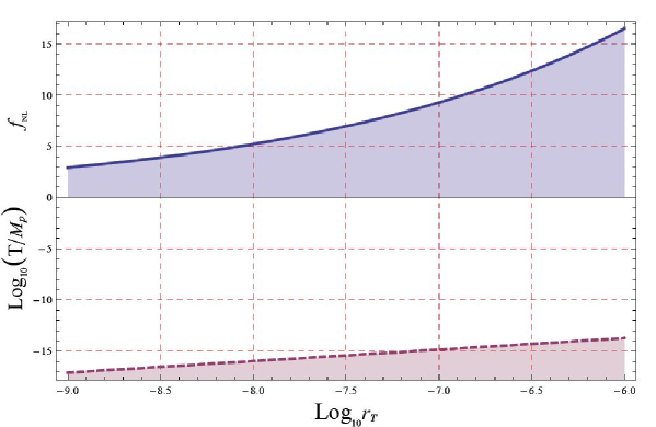
Figure 1: In this figure, we show the constraint (46) and (47). The up plate of the figure denotes the allowed region of $f_{NL}$ as a function of $r_{T}$ from (47). The shaded region is the allowed region. The down plate of the figure denotes the temperature when CDM decays which saturates the inequalities. In the shaded region, (47) is more strict than (46). In the unshaded region, (46) is more strict than (47).

For example, assume $f_{NL}$ is produced by the curvaton scenario. If $f_{NL}=50$, then $r_{T}>10^{-4}$. If the lower bound $r_{T}=10^{-4}$ is saturated, we get $T<10^{-11}M_{p}\sim 10^{7}$GeV. This constraint is not very tight for $m_{\rm CDM}$. However, it already rules out some CDM candidates within the curvaton scenario, such as invisible axions, magnetic monopoles and pyrgons.

On the other hand, if $f_{NL}=5$ then $r_{T}>10^{-8}$. This seems more natural in the small field inflation models. In this case, if the lower bound is saturated, we get $T<10^{-17}M_{p}\sim 10$GeV. This further rules out some dark matter candidates such as primordial black holes.

The inequality (46) is applicable until $f_{NL}\sim 1$. After that, other corrections for $f_{NL}$ begins to dominate. In this limit, $r_{T}>10^{-11}$. If this bound is saturated, then $T<10^{-19}M_{p}\sim 100$ MeV. This bound becomes borderline for LSP and quark nuggets type dark matter.

Finally, we would like to compare our result with a recent paper [31]. In [31], the author also aims to get a bound for the temperature of $f_{NL}$, $r_{T}$ and $T$. The difference between our work and [31] is that we use different methods to constrain the curvaton mass $m$. [31] uses the spectral index, which gives $m<0.1H_{*}$. While we use Eq. (42) to constrain $m$. This difference leads to different final results. In [31], the constraint takes the form

$$T<1.9\times 10^{-4}r_{T}^{5/4}f_{NL}^{-1}M_{p}\leavevmode\nobreak\ .$$ (48)

When $r_{T}^{1/2}<0.023f_{NL}$, our bound Eq. (46) is more tight than Eq. (48). When $r_{T}^{1/2}>0.023f_{NL}$, Eq. (48) is more tight.

6 Improved Treatment for Combined Inflaton and Curvaton Perturbations

Using the techniques developed in this paper, we are able to simplify some calculations for the mixed inflaton and curvaton scenario in the literature.

Note that the perturbations in the curvaton scenario (setting $\psi^{\rm(n)}=0$), isocurvaton scenario, and mixed inflaton and curvaton scenario are the same. The simplifications arises because we have chosen the $\delta\rho_{\varphi}=0$ gauge. This gauge choice, or rearranging the variables, can diagonalize the perturbation equations outside the horizon.

Consider the scenario investigated in [24], with the curvaton evolving in the radiation dominated era. Using the method in [24], one is forced to solve the Bessel equation with source term

$$\ddot{\delta\chi}^{\rm(n)}+3H\dot{\delta\chi}^{\rm(n)}+m^{2}\delta\chi^{\rm(n)}=4\dot{\chi}\dot{\psi}^{\rm(n)}-2m^{2}\chi\psi^{\rm(n)}\leavevmode\nobreak\ ,\leavevmode\nobreak\ \leavevmode\nobreak\ \leavevmode\nobreak\ H=\frac{1}{2t}\leavevmode\nobreak\ .$$ (49)

Although this equation can be solved analytically, it saves some calculation and be easier to generalize if one rewrites this equation in a sourceless manner. This simplification is just what we have done in Eq. (17), where we have considered a general potential for the curvaton and a general equation of state for the inflaton.

For the $m^{2}\chi^{2}$ type curvaton potential, Eq. (15) reads

$$\ddot{\delta\chi}+3H\dot{\delta\chi}+m^{2}\delta\chi=0\leavevmode\nobreak\ .$$ (50)

Note that this equation has the same form with the background evolution for $\chi$. So without solving any differential equations, we know that for the non-decaying solution,

$$\delta\chi=\frac{\chi}{\chi_{0}}\delta\chi_{0}\leavevmode\nobreak\ ,$$ (51)

where $\delta\chi_{0}$ is an integration constant. Use (15) to translate this result into the Newtonian gauge, we have

$$\delta\chi^{\rm(n)}=\frac{\chi}{\chi_{0}}\left(\delta\chi_{0}^{\rm(n)}-\dot{\chi}_{0}t_{0}\psi_{0}^{\rm(n)}\right)+t\dot{\chi}\psi^{\rm(n)}\leavevmode\nobreak\ .$$ (52)

Note that $\delta\chi_{0}^{\rm(n)}-\dot{\chi}_{0}t_{0}\psi_{0}^{\rm(n)}$ is just a constant, which can be redefined to $\delta\chi_{0}^{\rm(n)}$. Then we recover one of the key results in [24],

$$\delta\chi^{\rm(n)}=\frac{\chi}{\chi_{0}}\delta\chi_{0}^{\rm(n)}+t\dot{\chi}\psi^{\rm(n)}\leavevmode\nobreak\ ,$$ (53)

where we have not made any reference to the equation of state of the inflaton component. Other results for the $m^{2}\chi^{2}$ potential in [24] can be recovered similarly.

7 Generalizations for the Curvaton Model

In this section, we investigate the possibility for large negative $f_{NL}$ and nonlocal shape $f_{NL}$ in the curvaton model. This possibility can be realized by phantom curvaton and k-curvaton respectively. These models seem exotic, and not supported by any evidence so far. For example, the vacuum stability and the quantization problem in the phantom model are not solved. However, we investigate these models as pure phenomenological possibilities.

In reference [6], the WMAP5 data has been analyzed by two different methods. It is intriguing that the two methods prefer central values of $f_{NL}^{local}$ opposite in sign. In particular, both at the $95\%$ confidence level, the bispectrum analysis gives the best estimate $-9<f_{NL}^{local}<111$, while the analysis of Minkowski functionals prefers $-178<f_{NL}^{local}<64$ in contrast. It is still unclear why they are so different. However, if one naively disregards the bispectrum analysis for the moment, and takes seriously the central value from Minkowski functionals, we will be motivated to search for models with $f_{NL}^{local}\ll-1$. Let us see what will happen if the curvaton component is phantom-like [32]. In that case, the Eqs. (3) and (2) are still valid. However, now $\dot{\rho}_{\chi}>0$. So we have $r<0$, and $\zeta_{\chi}$ has the different sign from $\zeta$. It is well-known that a different sign in $\zeta$ should produce a different sign in $f_{NL}$. The calculation for $f_{NL}$ goes through in the phantom model, so when $|r|\ll 1$, we have

$$f_{NL}\sim\frac{1}{r}\ll-1\leavevmode\nobreak\ .$$ (54)

Although the bispectrum analysis of WMAP5 (which is widely taken as the best estimate) does not prefer a large negative $f_{NL}$, its lower bound $f_{NL}\simeq-9$ still allows for the phantomlike curvaton to live in a narrow space. From the opposite viewpoint, this can be another piece of evidence that nature disfavors phantom.

It is also worth to note that if the index of equation of state for the curvaton crosses $-1$ [33], then the non-Gaussianity produced by the curvaton model also crosses $-1$. To realize this possibility, one usually need more than one curvaton fields [34].

Now consider the k-curvaton possibility. If the curvaton has generalized kinetic terms, then the equilateral non-Gaussianity for the curvaton is also large. Similar to (9), we have

$$f_{NL}^{\rm(nonlocal)}=\frac{1}{r}f_{NL\chi}^{\rm(nonlocal)}\leavevmode\nobreak\ .$$ (55)

This amplification can easily produce very large equilateral non-Gaussianity. Note that $f_{NL}^{\rm(nonlocal)}\sim 1/c_{s}^{2}$. For example, if $1/c_{s}^{2}\simeq 5$, and $f_{NL}\simeq 50$, then we find $f_{NL}^{\rm(nonlocal)}\sim 250$. The experimental bound $-151<f_{NL}^{\rm(nonlocal)}<253$ (95% CL). If both large local and nonlocal $f_{NL}^{\rm(nonlocal)}$ is observed, the k-curvaton provides a satisfying explanation.

8 Conclusion and Discussion

To conclude, in this paper, we have investigated the isocurvaton scenario. We found that although the isocurvaton scenario possesses attractive features such as enhancement of non-Gaussianity and gravitational waves, the scenario can not be realized in the slow roll multi-field models. This no-go theorem can be extended to generalized kinetic terms with assumption $\Xi=0$. The techniques used in this paper can simplify some calculations in the mixed curvaton and inflaton scenario, providing an easier investigation for more general mixed perturbations.

We showed that the no-go result does no harm to the curvaton scenario. However, the experimental bound on non-Gaussianity, isocurvature perturbation, and gravitational waves provide a combined constraint (Eq. (46)) on the curvaton model.

We also investigated the phenomenology of phantom and kinetic curvatons. We showed that the phantom curvaton provides $f_{NL}\ll-1$, and the k-curvaton provides very large equilateral non-Gaussianity as well as the local non-Gaussianity.

Finally, let us discuss some possibilities to bypass the no-go theorem for isocurvaton. The following possibilities are not covered by the no-go theorem:

1. Adding interactions. It is reported from numerical calculation that interaction can suppress the super horizon perturbations [35]. It would be interesting to investigate whether similar mechanisms can realize the isocurvaton scenario.

2. Relaxing the slow roll condition for the isocurvaton field. It is challenging to construct fast rolling isocurvaton field which can fit the experimental results.

3. Other form of generalized kinetic terms, including separately generalized kinetic terms for inflaton and curvaton during inflation, high derivatives like the box term. The possibility $\Xi\neq 0$ is also worth investigating.

Appendix

We explain the notation we use, and review some well-known facts in the cosmological perturbation theory.

In the linear perturbation theory, assuming a flat universe ($K=0$), and without choosing any gauge, the metric for the scalar perturbation takes the form

$$g_{\mu\nu}=\left(\begin{array}[]{ccc}1+2\phi&-\beta_{,i}\\ -\beta_{,i}&-a^{2}((1-2\psi)\delta_{ij}+2E_{,ij})\end{array}\right)\leavevmode\nobreak\ ,$$ (56)

The Newtonian gauge is defined by setting

$$\beta^{\rm(n)}=0\leavevmode\nobreak\ ,\leavevmode\nobreak\ \leavevmode\nobreak\ \leavevmode\nobreak\ E^{\rm(n)}=0\leavevmode\nobreak\ .$$ (57)

For the $\delta\rho_{\varphi}=0$ gauge, the equation $\delta\rho_{\varphi}=0$ is just one gauge condition, and as in [36], we set the other gauge condition to be $E=0$. In this notation, the gauge transformation takes the form of Eq. (15).

The conserved quantity can be introduced as follows. Assuming that there is no energy change between $\varphi$ and $\chi$, the local energy conservation equation for $\varphi$ takes the form

$$H-\dot{\psi}=-\frac{1}{3}\frac{\partial_{t}(\rho_{\varphi}+\delta\rho_{\varphi})}{\rho_{\varphi}+\delta\rho_{\varphi}+p_{\varphi}+\delta p_{\varphi}}+{\cal O}\left[\left(\frac{k}{aH}\right)^{2}\right]\leavevmode\nobreak\ ,$$ (58)

Note that $H$ is a background quantity, and does not change with the spatial coordinate. If we assume the pressure is a function of only the energy density, then in the $\delta\rho_{\varphi}$ gauge, we have $\delta p_{\varphi}=0$. Thus the RHS of (58) is also independent of spacial coordinates. In order that (58) holds, $\dot{\psi}$ should also independent of spacial coordinates outside the horizon.

As a perturbation variable, $\psi$ should have no zero mode, so does $\dot{\psi}$. The only possibility is $\dot{\psi}=0$. We can define a conserved quantity

$$\zeta_{\varphi}=-\psi\big{|}_{\delta\rho_{\varphi}=0}\leavevmode\nobreak\ ,$$ (59)

which is conserved after horizon crossing. This conserved quantity can be rewritten in the gauge invariant form

$$\zeta_{\varphi}=-\psi-H\frac{\delta\rho_{\varphi}}{\dot{\varphi}}\leavevmode\nobreak\ .$$ (60)

From the same reasoning, there is also a gauge invariant conserved quantity for $\chi$,

$$\zeta_{\chi}=-\psi-H\frac{\delta\rho_{\chi}}{\dot{\chi}}\leavevmode\nobreak\ .$$ (61)

Note that these conserved quantities can be defined beyond the leading order perturbation theory. But we only need the leading order result for our purpose.

The above proof is under the assumption that in the $\delta\rho_{\varphi}=0$ gauge, we have $\delta p_{\varphi}=0$. This assumption is obviously true for fluids such as radiation and matter. It is also worth to note that this assumption is also true for inflaton after horizon crossing. This is because the above statement can be rewritten as the adiabatic condition

$$\dot{p}_{\varphi}\delta\rho_{\varphi}=\dot{\rho}_{\varphi}\delta p_{\varphi}\leavevmode\nobreak\ .$$ (62)

This condition can be checked directly using the Einstein equations in the $k\ll aH$ limit.

References

- [1] A. H. Guth, Phys. Rev. D23, 347 (1981).
- [2] A. D. Linde, Phys. Lett. B108, 389 (1982).
- [3] A. Albrecht, and P. J. Steinhardt, Phys. Rev. Lett. 48, 1220 (1982).
- [4] For earlier attemps on an inflationary model, see A. A. Starobinsky, JETP Lett. 30, 682 (1979) [Pisma Zh. Eksp. Teor. Fiz. 30 (1979) 719] ; A. A. Starobinsky, Phys. Lett. B91, 99 (1980).
- [5] A. D. Miller et al., Astrophys. J. 524, L1 (1999), astro-ph/9906421; P. de Bernardis et al., Nature 404, 955 (2000), astro-ph/0004404; S. Hanany et al., Astrophys. J. 524, L5 (2000), astro-ph/0005123; N. W. Halverson et al., Astrophys. J. 568, 38 (2002), astro-ph/0104489; B. S. Mason et al., Astrophys. J. 591, 540 (2003), astro-ph/0205384; A. Benoit et al., Astro. Astrophys. 399, L25 (2003), astro-ph/0210306; J. H. Goldstein et al., Astrophys. J. 599, 773 (2003), astro-ph/0212517;
- [6] E. Komatsu et al. [WMAP Collaboration], arXiv:0803.0547 [astro-ph].
- [7] V. Mukhanov, and G. Chibisov, JETP 33, 549 (1981).
- [8] A. H. Guth, and S.-Y. Pi, Phys. Rev. Lett. 49, 1110 (1982).
- [9] S. W. Hawking, Phys. Lett. B115, 295 (1982).
- [10] A. A. Starobinsky, Phys. Lett. B117, 175 (1982).
- [11] J. M. Bardeen, P. J. Steinhardt, and M. S. Turner, Phys. Rev. D28, 679 (1983).
- [12] E. Komatsu and D. N. Spergel, Phys. Rev. D 63, 063002 (2001) [arXiv:astro-ph/0005036]. E. Komatsu and D. N. Spergel, arXiv:astro-ph/0012197. E. Komatsu, arXiv:astro-ph/0206039.
- [13] A. D. Linde and V. F. Mukhanov, Phys. Rev. D 56, 535 (1997) [arXiv:astro-ph/9610219]. D. H. Lyth and D. Wands, Phys. Lett. B 524, 5 (2002) [arXiv:hep-ph/0110002].
- [14] K. Koyama, S. Mizuno, F. Vernizzi and D. Wands, JCAP 0711, 024 (2007) [arXiv:0708.4321 [hep-th]]. E. I. Buchbinder, J. Khoury and B. A. Ovrut, arXiv:0710.5172 [hep-th]. J. L. Lehners and P. J. Steinhardt, arXiv:0804.1293 [hep-th]. J. L. Lehners and P. J. Steinhardt, arXiv:0804.1293 [hep-th]. J. L. Lehners and P. J. Steinhardt, Phys. Rev. D 77, 063533 (2008) [arXiv:0712.3779 [hep-th]]. J. L. Lehners and P. J. Steinhardt, arXiv:0804.1293 [hep-th].
- [15] J. Garriga and V. F. Mukhanov, “Perturbations in k-inflation,” Phys. Lett. B 458, 219 1999 [arXiv:hep-th/9904176]. C. Armendariz-Picon, T. Damour and V. Mukhanov,“k-inflation,” Phys. Lett. B 458, 209 1999 [arXiv:hep-th/9904075].
- [16] E. Silverstein and D. Tong, “Scalar speed limits and cosmology: Acceleration from D-cceleration,” Phys. Rev. D 70:103505,2004 [arXiv:hep-th/0310221]. M. Alishahiha, E. Silverstein and D. Tong, “DBI in the Sky,” Phys. Rev. D 70:123505, 2004 [arXiv:hep-th/0404084]. X. Chen, Phys. Rev. D 71, 063506 (2005) [arXiv:hep-th/0408084]. X. Chen, JHEP 0508, 045 (2005) [arXiv:hep-th/0501184]. X. Chen, Phys. Rev. D 72, 123518 (2005) [arXiv:astro-ph/0507053]. K. Fang, B. Chen and W. Xue, Phys. Rev. D 77, 063523 (2008) [arXiv:0707.1970 [astro-ph]]. M. Li, T. Wang and Y. Wang, JCAP 0803, 028 (2008) [arXiv:0801.0040 [astro-ph]].
- [17] A. P. S. Yadav and B. D. Wandelt, arXiv:0712.1148 [astro-ph].
- [18] C. Gordon, D. Wands, B. A. Bassett and R. Maartens, Phys. Rev. D 63, 023506 (2001) [arXiv:astro-ph/0009131].
- [19] D. Seery and J. E. Lidsey, JCAP 0509, 011 (2005) [arXiv:astro-ph/0506056]. S. W. Li and W. Xue, arXiv:0804.0574 [astro-ph]. X. Gao, arXiv:0804.1055 [astro-ph].
- [20] B. Chen, M. Li, T. Wang and Y. Wang, Mod. Phys. Lett. A 22, 1987 (2007) [arXiv:astro-ph/0610514].
- [21] B. Chen, M. Li and Y. Wang, Nucl. Phys. B 774, 256 (2007) [arXiv:astro-ph/0611623].
- [22] M. S. Sloth, Mod. Phys. Lett. A 21, 961 (2006) [arXiv:hep-ph/0507315]. N. Bartolo, E. W. Kolb and A. Riotto, Mod. Phys. Lett. A 20, 3077 (2005) [arXiv:astro-ph/0507573].
- [23] A. Linde, V. Mukhanov and M. Sasaki, JCAP 0510, 002 (2005) [arXiv:astro-ph/0509015].
- [24] D. Langlois and F. Vernizzi, Phys. Rev. D 70, 063522 (2004) [arXiv:astro-ph/0403258].
- [25] D. H. Lyth, K. A. Malik and M. Sasaki, JCAP 0505, 004 (2005) [arXiv:astro-ph/0411220].
- [26] D. Wands, N. Bartolo, S. Matarrese and A. Riotto, Phys. Rev. D 66, 043520 (2002) [arXiv:astro-ph/0205253]. B. J. W. van Tent, Class. Quant. Grav. 21, 349 (2004) [arXiv:astro-ph/0307048]. C. T. Byrnes and D. Wands, Phys. Rev. D 74, 043529 (2006) [arXiv:astro-ph/0605679].
- [27] D. Langlois and S. Renaux-Petel, arXiv:0801.1085 [hep-th].
- [28] H. X. Yang and H. L. Ma, arXiv:0804.3653 [hep-th].
- [29] Q. G. Huang, arXiv:0801.0467 [hep-th].
- [30] D. H. Lyth, C. Ungarelli and D. Wands, Phys. Rev. D 67, 023503 (2003) [arXiv:astro-ph/0208055].
- [31] M. Beltran, arXiv:0804.1097 [astro-ph].
- [32] R. R. Caldwell, Phys. Lett. B 545, 23 (2002) [arXiv:astro-ph/9908168].
- [33] B. Feng, X. L. Wang and X. M. Zhang, Phys. Lett. B 607, 35 (2005) [arXiv:astro-ph/0404224].
- [34] J. Q. Xia, Y. F. Cai, T. T. Qiu, G. B. Zhao and X. Zhang, arXiv:astro-ph/0703202.
- [35] T. Multamaki, J. Sainio and I. Vilja, arXiv:astro-ph/0609019.
- [36] J.Maldacena, “Non-Gaussian features of primordial fluctuations in single field inflationary models,” JHEP 0305:013,2003 [arXiv:astro-ph/0210603].