A new molecular dynamics calculation and its application to the spectra of light and strange baryons

Abstract

A new approach based on antisymmetrized molecular dynamics is proposed to correctly take account of the many-body correlation. We applied it to the spectra of low-lying, light and strange baryons. The inclusion of the quark-quark correlation is vital to predict the precise spectra, and the semi-relativistic kinematics is also important to correct the level ordering. The baryon spectra calculated by the present method is as precise as the Faddeev calculation.

Although recent lattice calculations based on Quantum Chromodynamics (QCD) start providing reliable hadron spectra, it is still difficult to obtain precise, detailed predictions of the physical states lattice . Thus, QCD-inspired, effective models are still useful to get some insight into many phenomena of hadronic systems. The central issue to be addressed is then the quantitative description of low-energy phenomena, e.g., hadron spectra, baryon-baryon interactions, in-medium change of hadron properties saito , etc.

Among QCD-inspired models, the simplest approach is the nonrelativistic (NR), constituent quark model (CQM), and it is doubtlessly successful in describing the ground-state properties of hadrons and baryon-baryon interactions at low energies cqm . There are, however, some obscure problems such as the level-ordering problem in excited hadron spectra, etc. In addition to ordinary mesons and baryons, the (NR) CQM is also applied to exotic states, e.g., multiquark states including pentaquarks, non $q{\bar{q}}$-mesons (tetraquarks tetra ), etc.

The QCD lagrangian for massless up and down quarks is chirally symmetric, and the axial symmetry is spontaneously broken as evidenced in the absence of parity doublets in the low-mass hadron spectra. This implies the existence of the massless Nambu-Goldstone (NG) bosons, e.g., the pions. The non-zero pion mass is then a consequence of the fact that the light quark has a small mass, which gives the explicit symmetry breaking. Thus, one arrives at a low-energy scenario that consists of the NG bosons and constituent quarks (with a rather massive, constituent quark mass in the NG phase) interacting via a force governed by spontaneously broken, approximate chiral symmetry. Thus, it is of very importance to take into account the effect of the NG-boson exchange as well as the usual one-gluon-exchange (OGE) force in the CQM. Note that multigluon degrees of freedom can be elminated by introducing a confining potential. Furthermore, the relativistic effect may be vital to produce the hadron spectra, because the quarks move in the region of the hadron size.

There are a lot of model calculations to study hadron spectra, baryon-baryon interactions, etc cqm ; SVM1 ; ESP1 ; ESP3 ; ESP4 . In the calculation of baryon spectra, the most precise method may be based on the Faddeev equations for the three constituent quarks ESP3 . However, for multiquark states like the exotic hadrons, it is quite difficult to perform such precise calculations. Thus, it is very important and useful to construct a powerful method which allows us to precisely calculate the wavefunction even for multiquark states.

Molecular dynamics (MD) is very successful in treating many-body systems. In particular, fermionic molecular dynamics (FMD) was first developed by Feldmeier fmd to describe the ground states of atomic nuclei and heavy ion reactions in the energy regime below particle production. Antisymmetrized molecular dynamics (AMD) ONO ; ENYO1 is very similar to FMD with respect to the choice of the trial state. In the past decade, AMD has been applied to various studies of light or medium nuclei ENYO21 . In AMD, it is not necessary to take any model assumption (like shell, cluster, etc.), and the AMD wavefunction can simultaneously describe a variety of nuclear structure by following the variational principle.

However, AMD has not yet been successfully applied to a few-body system, because the trial wavefunction in AMD is given by the Slater determinant of single-particle, gaussian wave packets and hence the correlation among nucleons is missing. To improve this weak point, some of the present authors have recently proposed a modified version of AMD, in which the Jacobi coordinates and the generator-coordinate method (GCM) are introduced to describe the correlation JAMD . We here refer to this method as the Jacobi-coordinate-basis AMD (JAMD). In JAMD, one can easily treat the many-body correlations. Furthermore, it is possible to extract the center-of-mass (c.m.) wavefunction and remove the zero-point energy.

In this paper, we apply the present method to the SU(3) octet- and decuplet-baryon spectra, and compare the JAMD result with that of the simple AMD or the Faddeev result to illustrate how this method is useful.

In AMD, the wavefunction of $A$-quark system with definite ($\pm$) parity, $|\Psi^{\pm}\rangle$, is given by ONO ; ENYO1

$$|\Psi^{\pm}\rangle=|{\mathcal{C}}\rangle\sum_{i=1}^{A!}|\Phi_{p_{i}}^{\pm}\rangle|{\mathcal{S}}_{p_{i}}\rangle|{\mathcal{F}}_{p_{i}}\rangle,$$ (1)

where $|\Phi_{p_{i}}^{\pm}\rangle$, $|{\mathcal{S}}_{p_{i}}\rangle$, $|{\mathcal{F}}_{p_{i}}\rangle$ and $|{\mathcal{C}}\rangle$ are, respectively, the spatial, spin, flavor and color wavefunctions. The color wavefunction is then antisymmetrized as

$$|{\mathcal{C}}\rangle=\sum_{i=1}^{A!}{\rm sgn}(p_{i})|m^{c}_{p_{i}(1)}m^{c}_{p_{i}(2)}\cdots m^{c}_{p_{i}(A)}\rangle,$$ (2)

where $m^{c}$ specifies the color and sgn$(p_{i})$ is the sign of the permutation $p_{i}\,(i=1,2,\,\cdots,\,A!)$:

$$p_{i}=\left(\begin{array}[]{ccccc}1&2&3&\dots&A\\ j_{1}&j_{2}&j_{3}&\dots&j_{A}\end{array}\right)\equiv\left(\begin{array}[]{ccccc}1&2&3&\dots&A\\ p_{i}(1)&p_{i}(2)&p_{i}(3)&\dots&p_{i}(A)\end{array}\right).$$ (7)

Because the color wavefunction is already antisymmetrized, the other wavefunctions must be symmetrized in Eq.(1). The spatial wavefunction is then given by the product of a single-particle wavefunction

$$|\Phi_{p_{i}}^{\pm}\rangle=(1\pm P)|\phi_{1}(p_{i}(1))\phi_{2}(p_{i}(2))\dots\phi_{A}(p_{i}(A))\rangle,$$ (8)

where $1\pm P$ is the parity projection operator and the $i$-th single-particle wavefunction (at ${\vec{r}}_{i}$) is given by a gaussian function

$$\phi_{i}(j)=\exp[-\nu({\vec{r}}_{i}-{\vec{Z}}_{j})^{2}],$$ (9)

with ${\vec{Z}}$ the center of the wave packet and $\nu$ a variational parameter for its width. The spin wavefunction is expressed as

$$|{\mathcal{S}}_{p_{i}}\rangle=\sum_{m^{s}=\uparrow,\downarrow}c^{s}_{p_{i}(1)\cdots p_{i}(A)}|m^{s}_{p_{i}(1)}\cdots m^{s}_{p_{i}(A)}\rangle,$$ (10)

where the coefficient, $c^{s}$, is a variational parameter. However, since, for the low-lying baryon states, the spin-flavor structure ($|{\mathcal{S}}_{p_{i}}\rangle|{\mathcal{F}}_{p_{i}}\rangle$ in Eq.(1)) can be given by SU(6) symmetry, we here use it to reduce the computation time.

In JAMD, the spatial wavefunction is expressed in terms of gaussian functions with the Jacobi coordinates (${\vec{\rho}}_{i};\,i=1,2,\,\cdots,\,A$) JAMD . Then, the usual single-particle coordinates, ${\vec{r}}_{i}$, can be related to the Jacobi coordinates through ${\vec{\rho}}_{i}=\sum_{k=1}^{A}K_{ik}{\vec{r}}_{k}$, where the matrix $K$ is given by SVM2

$$K=\left(\begin{array}[]{ccccc}1&-1&0&\cdots&0\\ \frac{m_{1}}{m_{12}}&\frac{m_{2}}{m_{12}}&-1&\cdots&0\\ \vdots&&&\vdots\\ \frac{m_{1}}{m_{12\cdots A-1}}&\frac{m_{2}}{m_{12\cdots A-1}}&\cdots&\cdots&-1\\ \frac{m_{1}}{m_{12\cdots A}}&\frac{m_{2}}{m_{12\cdots A}}&\cdots&\cdots&\frac{m_{A}}{m_{12\cdots A}}\\ \end{array}\right),$$ (16)

where $m_{12\cdots k}=m_{1}+m_{2}+\cdots+m_{k}$ and $m_{i}$ is the mass of the $i$-th particle. The center of the gaussian wave packet, ${\vec{X}}_{i}$, in the JAMD wavefunction is also related to ${\vec{Z}}_{j}$ using the $K$ matrix JAMD . Thus, the spacial part of the JAMD wavefunction, $\Phi^{J}$, with the width, $\nu_{ij}^{J}$, can be expressed in terms of the usual coordinates as

$$\Phi^{J} = \exp\Big{[}-\sum_{i,j=1}^{A}\nu_{ij}^{J}({\vec{\rho}}_{i}-{\vec{X}}_{i})\cdot({\rho}_{j}-{\vec{X}}_{j})\Big{]}=\exp\Big{[}-\sum_{i,j=1}^{A}\nu_{ij}({\vec{r}}_{i}-{\vec{Z}}_{i})\cdot({\vec{r}}_{j}-{\vec{Z}}_{j})\Big{]}$$ (17)

$$= \exp\Big{[}-\frac{1}{2}\sum_{i,j=1}^{A}\tilde{\nu}_{ij}\Big{\{}({\vec{r}}_{i}-{\vec{Z}}_{i})-({\vec{r}}_{j}-{\vec{Z}}_{j})\Big{\}}^{2}-\nu_{AA}({\vec{\rho}_{A}}-{\vec{X}}_{A})^{\,2}\Big{]},$$

where each element of the width matrix, ${\tilde{\nu}}_{ij}$, is treated as a variational parameter, and $\nu^{J}_{ij}$, $\nu_{ij}$ and ${\tilde{\nu}}_{ij}\ (i,j=1,2,\,\cdots,\,A)$ satisfy the following relation:

$$\nu_{ij}=\sum_{k,l=1}^{A}\nu_{kl}^{J}K_{ki}K_{lj}=\sum_{k=1}^{A}\tilde{\nu}_{ik}\delta_{ij}-\tilde{\nu}_{ij}+\frac{m_{i}m_{j}}{M^{2}}\nu_{AA}.$$ (18)

Now let us apply the JAMD method to the SU(3) octet and decuplet baryons. The hamiltonian is given by

$$H=T+V_{\chi}(\vec{r}_{ij})+V_{\rm OGE}(\vec{r}_{ij})+V_{\rm CON}(\vec{r}_{ij}),$$ (19)

where $T$ is the kinetic-energy term. In this paper, as well as the NR form, we consider the semi-relativistic (SR) form to take into account the relativistic effect:

$$T=\left\{\begin{array}[]{l>{$}l<{$}}\frac{1}{2}\sum_{i>j}^{A}\frac{m_{i}+m_{j}}{m_{i}m_{j}}({\vec{p}}_{j}-{\vec{p}}_{i})^{2}+\sum_{i=1}^{A}m_{i}&\ \ \ for NR,\\ \sum_{i=1}^{A}\sqrt{{\vec{p}}_{i}^{\ 2}+m_{i}^{2}}&\ \ \ for SR,\end{array}\right.$$ (22)

where $m_{i}$ is the $i$-th quark mass.

The potential generated by the exchanges of the NG bosons ($\pi,K,\eta$) and the $\sigma$ meson is given by $V_{\chi}({\vec{r}}_{ij})=V_{\pi}({\vec{r}}_{ij})+V_{\sigma}({\vec{r}}_{ij})+V_{K}({\vec{r}}_{ij})+V_{\eta}({\vec{r}}_{ij})$ ESP1 ; ESP3 , where

$$V_{\pi}({\vec{r}}_{ij}) = \frac{g_{ch}^{2}}{4\pi}\frac{m_{\pi}^{3}}{12m_{i}m_{j}}\frac{\Lambda_{\pi}^{2}}{\Lambda_{\pi}^{2}-m_{\pi}^{2}}\Big{[}Y(m_{\pi}r_{ij})-\frac{\Lambda_{\pi}^{3}}{m_{\pi}^{3}}Y(\Lambda_{\pi}r_{ij})\Big{]}({\vec{\sigma}}_{i}\cdot{\vec{\sigma}}_{j})\sum_{a=1}^{3}(\lambda_{i}^{a}\cdot\lambda_{j}^{a}),$$ (23)

$$V_{\sigma}({\vec{r}}_{ij}) = -\frac{g_{ch}^{2}}{4\pi}\frac{\Lambda_{\sigma}^{2}}{\Lambda_{\sigma}^{2}-m_{\sigma}^{2}}m_{\sigma}{\Big{[}Y(m_{\sigma}r_{ij})-\frac{\Lambda_{\sigma}}{m_{\sigma}}Y(\Lambda_{\sigma}r_{ij})}{\Big{]}},$$ (24)

$$V_{K}({\vec{r}}_{ij}) = \frac{g_{ch}^{2}}{4\pi}\frac{m_{K}^{3}}{12m_{i}m_{j}}\frac{\Lambda_{K}^{2}}{\Lambda_{K}^{2}-m_{K}^{2}}{\Big{[}Y(m_{K}r_{ij})-\frac{\Lambda_{K}^{3}}{m_{K}^{3}}Y(\Lambda_{K}r_{ij})}{\Big{]}}({\vec{\sigma}}_{i}\cdot{\vec{\sigma}}_{j})\sum_{a=4}^{7}(\lambda_{i}^{a}\cdot\lambda_{j}^{a}),$$ (25)

$$V_{\eta}({\vec{r}}_{ij}) = \frac{g_{ch}^{2}}{4\pi}\frac{m_{\eta}^{3}}{12m_{i}m_{j}}\frac{\Lambda_{\eta}^{2}}{\Lambda_{\eta}^{2}-m_{\eta}^{2}}{\Big{[}Y(m_{\eta}r_{ij})-\frac{\Lambda_{\eta}^{3}}{m_{\eta}^{3}}Y(\Lambda_{\eta}r_{ij})}{\Big{]}}({\vec{\sigma}}_{i}\cdot{\vec{\sigma}}_{j})\Theta_{P},$$ (26)

with ${\vec{r}}_{ij}={\vec{r}}_{i}-{\vec{r}}_{j}$, $\lambda^{a}$ the SU(3) generator, $g_{ch}$ the chiral coupling constant, $\Lambda_{\pi,\sigma,K,\eta}$ the cutoff parameter, $Y(mr)$ the Yukawa function and $\Theta_{P}(=\cos\theta_{P}(\lambda_{i}^{8}\cdot\lambda_{j}^{8})-\sin\theta_{P})$ the mixing term for considering the physical $\eta$. The masses of the NG bosons are denoted by $m_{\pi}$, $m_{K}$ and $m_{\eta}$. The $\sigma$ mass is chosen to be $m_{\sigma}^{2}\sim m_{\pi}^{2}+4m_{u,d}^{2}$ ESP3 .

The potential due to the OGE is ESP1 ; ESP3

$$V_{\rm OGE}({\vec{r}}_{ij}) = \frac{1}{4}\,\alpha_{s}{\vec{\lambda}}_{i}\cdot{\vec{\lambda}}_{j}\frac{1}{r_{ij}}+\frac{1}{4}\,\alpha_{s}{\vec{\lambda}}_{i}\cdot{\vec{\lambda}}_{j}\frac{1}{m_{i}m_{j}}\frac{e^{-r_{ij}/r_{0}}}{r_{ij}r_{0}^{2}}$$ (29)

$$\times\left\{\begin{array}[]{l>{$}l<{$}}\frac{1}{6}{\vec{\sigma}}_{i}\cdot{\vec{\sigma}}_{j}&\ \ for NR,\\ \frac{1}{4}\Big{(}1+\frac{2}{3}{\vec{\sigma}}_{i}\cdot{\vec{\sigma}}_{j}\Big{)}&\ \ for SR ,\end{array}\right.$$

with $\alpha_{s}$ the quark-gluon coupling constant and $r_{0}$ a parameter to be fixed from the data. Note that in Ref. ESP3 $r_{0}$ is chosen to be a function of the quark mass. However, in the SR calculation, we can obtain a good result of the baryon spectra even if $r_{0}$ is assumed to be constant (see Table 2).

The confining potential is given by ESP1 ; ESP3

$$V_{\rm{CON}}({\vec{r}}_{ij})=-C_{\rm{3q}}-\left\{\begin{array}[]{l>{$}l<{$}}a_{c}\,(1-e^{-\mu_{c}r_{ij}})({\vec{\lambda}}_{i}^{c}\cdot{\vec{\lambda}}_{j}^{c})&\ \ for NR,\\ a_{c}\,r_{ij}({\vec{\lambda}}_{i}^{c}\cdot{\vec{\lambda}}_{j}^{c})&\ \ for SR,\end{array}\right.$$ (32)

with $a_{c}$ the effective confinement strength, $\mu_{c}$ a parameter for the screening effect and $C_{3q}$ a parameter for taking account of the vacuum energy.

To perform the numerical calculation, we use the following identities:

$$\sqrt{p^{2}+m^{2}} = \sqrt{C}-\frac{1}{\sqrt{\pi}}\int_{0}^{\infty}\frac{1}{w^{2}}(e^{-(p^{2}+m^{2})w^{2}}-e^{-Cw^{2}})dw,$$ (33)

$$\frac{e^{-ar}}{r} = \frac{2}{\sqrt{\pi}}\int_{0}^{\infty}e^{-\frac{a^{2}}{4w^{2}}-r^{2}w^{2}}dw,$$ (34)

where $C$ is an arbitrary, real number. Using these formulas, one can expand the SR kinetic energy and the potentials in terms of gaussian functions.

Varying the variational parameters included in the JAMD wavefunction, the total energy of the system

$$E^{\pm}=\frac{\langle\Psi^{\pm}|H|\Psi^{\pm}\rangle}{\langle\Psi^{\pm}|\Psi^{\pm}\rangle}$$ (35)

is minimized. To perform such calculation, it is very convenient to use the frictional cooling method ENYO1 , which provides the time-development equations for the center, ${\vec{Z}}_{i}$, and the width parameter, $\tilde{\nu}_{ij}$, as

$$\frac{dZ_{i\lambda}}{dt} = \mu\frac{\partial E^{\pm}}{\partial Z^{*}_{i\lambda}}\ \ \ \ \ (i=1,2,\cdots,A;\ \lambda=x,y,z),$$ (36)

$$\frac{d\tilde{\nu}_{ij}}{dt} = \mu^{\prime}\frac{\partial E^{\pm}}{\partial\tilde{\nu}_{ij}}\ \ \ \ \ (i>j=1,2,\cdots,A),$$ (37)

where $\mu$ and $\mu^{\prime}$ are arbitrary, negative real numbers. After sufficient time steps for the cooling, we can obtain the optimized wavefunction as a function of ${\vec{Z}}_{i}$ and $\tilde{\nu}_{ij}$. We refer to this wavefunction as $\Psi^{{\rm JAMD-I}}$.

In contrast, we consider another wavefunction which is given by superposing the JAMD wavefunction $\Psi$ ($\pm$ is suppressed here) with ${\vec{Z}}_{i}$ calculated in $\Psi^{{\rm JAMD-I}}$ but with ${\tilde{\nu}_{ij}}$ supplied by a geometrical progression JAMD or a random number generator SVM2 . In this case, ${\vec{Z}}_{i}$ and ${\tilde{\nu}_{ij}}$ are no longer the variational parameters. Then, the wavefunction (we call this $\Psi^{{\rm JAMD-II}}$) is given by

$$\Psi^{\rm{JAMD-II}}=c\Psi({\vec{Z}}_{i},\tilde{\nu}_{ij})+c^{\prime}\Psi({\vec{Z}}_{i},{\tilde{\nu}^{\prime}}_{ij})+c^{\prime\prime}\Psi({\vec{Z}}_{i},{\tilde{\nu}^{\prime\prime}}_{ij})+\cdots,$$ (38)

where, instead of ${\vec{Z}}_{i}$ and ${\tilde{\nu}_{ij}}$, the coefficients, $c,c^{\prime\prime},c^{\prime\prime\prime},\cdots$, are now variational parameters, and they are determined by the Hill-Wheeler equation

$$\delta(\langle\Psi^{\rm{JAMD-II}}|H|\Psi^{\rm{JAMD-II}}\rangle-E\langle\Psi^{\rm{JAMD-II}}|\Psi^{\rm{JAMD-II}}\rangle)=0.$$ (39)

Table 1: Values of the parameters.

		NR ESP3				SR ESP1
Fixed
$u$, $d$ quark mass	$m_{u}=m_{d}$ (MeV)	313				313
NG bosons	$m_{\pi}\,$(fm-1)	0.70				0.70
	$m_{\eta}\,$(fm-1)	2.77				2.77
	$m_{K}\,$(fm-1)	2.51				2.51
$\sigma$ meson mass	$m_{\sigma}\,$(fm-1)	3.42				3.42
cutoff	$\Lambda_{\pi}=\Lambda_{\sigma}$  (fm-1)	4.20				2.20
	$\Lambda_{\eta}=\Lambda_{K}$  (fm-1)	5.20				2.70
coupling constant	$g^{2}_{ch}/(4\pi)$ (fm-1)	0.54				0.54
mixing angle	$\theta_{P}\,$(∘)	$-15$				$-15$
confinement	$a_{c}$  (MeV)	230				110
	$\mu_{c}$  (fm-1)	0.70				—
OGE	$r_{0}$	0.35				0.74
		NR				SR
		AMD	JAMD-I	JAMD-II		JAMD-I	JAMD-II
Free
$s$ quark mass	$m_{s}$ (MeV)	598	587	554		562	525
vacuum	$C_{3q}$  (MeV)	333	346	372		128	177
OGE	$\alpha_{s}$	0.858	0.761	0.540		0.775	0.500

Now we are in a position to show the numerical result for the baryon spectra. The parameters in the present calculation are listed in Table 1. In case of the NR calculation, we take the parameters given in Ref. ESP3 . We assume that the value of $r_{0}$ in $V_{\rm OGE}$ is flavor-independent. In the SR calculation, referring to Ref. ESP1 , we determine the parameters in the potentials. Finally, three parameters, $C_{3q}$, $\alpha_{s}$ and $m_{s}$, remain. Then, the nucleon ($N$) mass is reproduced by tuning $C_{3q}$, while $\alpha_{s}$ is chosen so as to fit the $N$-$\Delta$ mass difference. The strange-quark mass, $m_{s}$, is determined from fit to the $N$-$\Omega$ mass difference.

Table 2: Calculated baryon masses (in MeV). The excited baryons are calculated in the JAMD-II.

State		NR					SR			Experiment
		AMD	JAMD-I	JAMD-II	FaddeevESP3		JAMD-I	JAMD-II
$N(1/2^{+})$		939	939	939	939		939	939		939
$N(1/2^{-})$		1481	1460	1409	1411		1522	1480		1553
$N^{*}(1/2^{+})$		—	—	1423	1435		—	1409		1440
$\Delta(3/2^{+})$		1230	1232	1234	1232		1235	1236		1232
$\Delta^{*}(3/2^{+})$		—	—	1589	—		—	1601		1600
$\Sigma(1/2^{+})$		1315	1264	1246	1213		1244	1214		1193
$\Sigma^{*}(1/2^{+})$		—	1400	1678	1644		—	1553		1660
$\Sigma(3/2^{+})$		1435	1404	1396	1398		1384	1382		1385
$\Sigma(1/2^{-})$		1722	1639	1631	1598		1726	1678		1620
$\Lambda(1/2^{+})$		1166	1160	1135	1122		1139	1120		1116
$\Xi(1/2^{+})$		1418	1401	1375	1351		1374	1359		1318
$\Omega(3/2^{+})$		1673	1673	1673	1650		1671	1670		1672

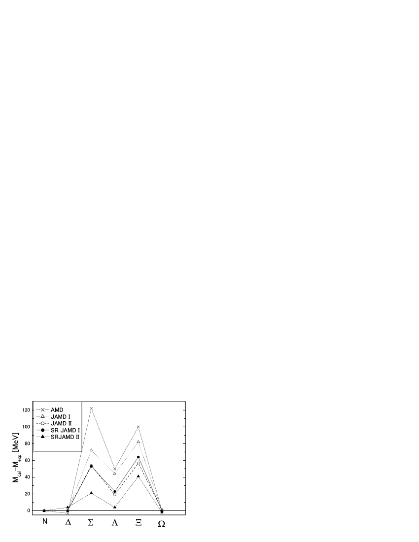
Figure 1: Difference between the calculated mass and the experimental value.

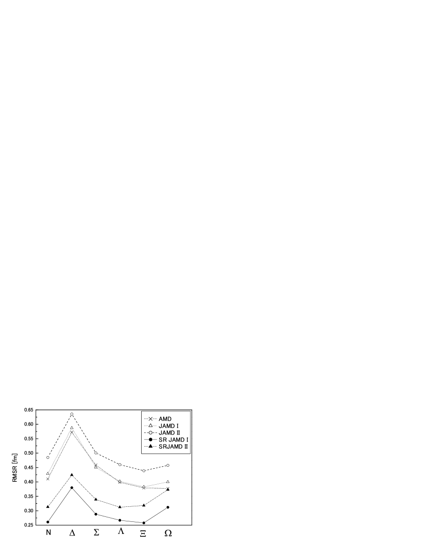
Figure 2: Root-mean-square radius.

In Table 2, we present the results of AMD and JAMD, and compare them with the Faddeev calculation ESP3 . Furthermore, in Fig. 1, the deviation of the calculated, ground-state mass from the observed one is shown to illustrate the model dependence of the baryon masses. The present result clearly show that the JAMD approach is much better than AMD in describing the baryon spectra. This fact implies the importance of the quark-quark correlation in the baryon structure. In particular, within the NR calculation, the JAMD-II result is very close to the spectra given by the Faddeev approach.

In the SR calculation, the present approach again reproduces the spectra of the low-lying light and strange baryons very well. In particular, the JAMD-II can provides the precise result as in the Faddeev calculation. It is also remarkable that the level ordering of the lowest positive- and negative-parity states in the nucleon spectra can be correctly reproduced in the SR calculation SVM1 ; ESP1 . This fact certainly results from the relativistic kinematics, because, in the NR calculation, we cannot produce the correct level ordering. It is, however, necessary to study further to obtain a quantitative result of $N(1/2^{-})$ and $N^{*}(1/2^{+})$.

In Fig 2, we show the root-mean-square (rms) radius of the baryon calculated using the quark wavefunction. It is noticeable that the rms radius is very small in the SR calculation, whereas, in the NR calculation, it has the reasonable size. It should, however, be noticed that the meson cloud surrounding the baryon core contributes to the present value additionally. The tendency of the rms radii of the low-lying baryons does not depend much on the choice of the model.

In summary, we have proposed a new approach of molecular dynamics based on AMD, in which the many-body correlation can be considered correctly. In this paper, we applied it to the spectra of the low-lying, light and strange baryons. It is shown that the inclusion of the quark-quark correlation is very vital to predict the precise spectra, and that the relativistic effect is also important to correct the level ordering. The JAMD approach can reproduce the baryon spectra very well. In particular, the spectra given by the JAMD-II calculation are very similar to the Faddeev result. Although we study the ordinary baryons in this paper, the present approach is very promising even in the calculation of a system containing four, five or more quarks. Thus, it is very intriguing to calculate the spectra of exotic hadrons like pentaquark, tetraquark, etc exotic .