Abstract

One of the most surprising consequences of quantum mechanics is the nonlocal correlation of a multi-particle system observable in joint-detection of distant particle-detectors. Ghost imaging is one of such phenomena. Taking a photograph of an object, traditionally, we need to face a camera to the object. But with ghost imaging, we can image the object by pointing a CCD camera towards the light source, rather than towards the object. Ghost imaging is reproduced at quantum level by a non-factorizable point-to-point image-forming correlation between two photons. Two types of ghost imaging have been experimentally demonstrated since 1995. Type-one ghost imaging uses entangled photon pairs as the light source. The non-factorizable image-forming correlation is the result of a nonlocal constructive-destructive interference among a large number of biphoton amplitudes, a nonclassical entity corresponding to different yet indistinguishable alternative ways for the photon pair to produce a joint-detction event between distant photodetectors. Type-two ghost imaging uses chaotic light. The type-two non-factorizable image-forming correlation is caused by the superposition between paired two-photon amplitudes, or the symmetrized effective two-photon wavefunction, corresponding to two different yet indistinguishable alternative ways of triggering a join-detection event by two independent photons. The multi-photon interference nature of ghost imaging determines its peculiar features: (1) it is nonlocal; (2) its imaging resolution differs from that of classical; and (3) the type-two ghost image is turbulence-free. Ghost imaging has attracted a great deal of attention, perhaps due to these features for certain applications. Achieving these features, the realization of nonlocal multi-photon interference is a necessary condition. Classical simulations, such as the man-made factorizable speckle-speckle correlation, can never have such features.

1 Introduction

Assuming an object that is either self-luminous or externally illuminated, imagining each point on the object surface as a point radiation sub-source, each point sub-source will emit spherical waves to all possible directions. How much chance do we expect to have a spherical wave collapsing into a point or a “speckle” by free propagation? Obviously, the chance is zero unless an imaging system is applied. The concept of optical imaging was well developed in classical optics for this purpose. Figure 1 schematically illustrates a standard imaging setup. In this setup an object is illuminated by a radiation source, an imaging lens is used to focus the scattered and reflected light from the object onto an image plane which is defined by the “Gaussian thin lens equation”

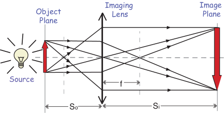
Figure 1: Optical imaging: a lens produces an image of an object in the plane defined by the Gaussian thin-lens equation $1/s_{i}+1/s_{o}=1/f$. Image formation is based on a point-to-point relationship between the object plane and the image plane. All radiations emitted from a point on the object plane will “collapse” to a unique point on the image plane.

$$\frac{1}{s_{i}}+\frac{1}{s_{o}}=\frac{1}{f},$$ (1)

where $s_{o}$ is the distance between the object and the imaging lens, $s_{i}$ the distance between the imaging lens and the image plane, and $f$ the focal length of the imaging lens. Basically this equation defines a point-to-point relationship between the object plane and the image plane: any radiation starting from a point on the object plane will “collapse” to a unique point on the image plane. It is not difficult to see from Fig. 1 that the point-to-point relationship is the result of constructive-destructive interference. The radiation fields coming from a point on the object plane will experience equal distance propagation to superpose constructively at one unique point on the image plane, and experience unequal distance propagations to superpose destructively at all other points on the image plane. The use of the imaging lens makes this constructive-destructive interference possible.

A perfect point-to-point image-forming relationship between the object and image planes produces a perfect image. The observed image is a reproduction, either magnified or demagnified, of the illuminated object, mathematically corresponding to a convolution between the object distribution function $|A(\vec{\rho}_{o})|^{2}$ (aperture function) and a $\delta$-function which characterizes the perfect point-to-point relationship between the object and image planes:

$$I(\vec{\rho}_{i})=\int_{obj}d\vec{\rho}_{o}\,\big{|}A(\vec{\rho}_{o})\big{|}^{2}\,\delta(\vec{\rho}_{o}+\frac{\vec{\rho}_{i}}{m})$$ (2)

where $I(\vec{\rho}_{i})$ is the intensity in the image plane, $\vec{\rho}_{o}$ and $\vec{\rho}_{i}$ are 2-D vectors of the transverse coordinates in the object and image planes, respectively, and $m=s_{i}/s_{o}$ is the image magnification factor.

In reality, limited by the finite size of the imaging system, we may never obtain a perfect point-to-point correspondence. The incomplete constructive-destructive interference turns the point-to-point correspondence into a point-to-“spot” relationship. The $\delta$-function in the convolution of Eq. (2) will be replaced by a point-spread function:

$$I(\vec{\rho}_{i})=\int_{obj}d\vec{\rho}_{o}\,\big{|}A(\vec{\rho}_{o})\big{|}^{2}\,somb^{2}\big{[}\frac{R}{s_{o}}\,\frac{\omega}{c}\big{|}\vec{\rho}_{o}+\frac{\vec{\rho}_{i}}{m}\big{|}\big{]},$$ (3)

where the sombrero-like function, or the Airy disk, is defined as

$$somb(x)=\frac{2J_{1}(x)}{x},$$

and $J_{1}(x)$ is the first-order Bessel function, and $R$ the radius of the imaging lens, and $R/s_{o}$ is known as the numerical aperture of the imaging system. The sombrero-like point-spread function, or the Airy disk, defines the spot size on the image plane that is produced by the radiation coming from point $\vec{\rho}_{o}$. It is clear from Eq. (3) that a larger imaging lens and shorter wavelength will result in a narrower point-spread function, and thus a higher spatial resolution of the image. The finite size of the spot determines the spatial resolution of the imaging system.

Type-one and type-two ghost imaging, in certain aspects, exhibit a similar point-to-point imaging-forming function as that of classical except the ghost image is reproducible only in the joint-detection between two independent photodetectors, and the point-to-point imaging-forming function is in the form of second-order correlation,

$$R_{12}(\vec{\rho}_{i})=\int_{obj}d\vec{\rho}_{o}\,\big{|}A(\vec{\rho}_{o})\big{|}^{2}\,G^{(2)}(\vec{\rho}_{o},\vec{\rho}_{i}),$$ (4)

where $R_{12}(\vec{\rho}_{i})$ is the joint-detection counting rate between photodetectors $D_{1}$ and $D_{2}$. Mathematically, the convolution is taken between the aperture function of the object $\big{|}A(\vec{\rho}_{o})\big{|}^{2}$ and a nontrivial poin-to-point second-order correlation function $G^{(2)}(\vec{\rho}_{o},\vec{\rho}_{i})$, corresponding to the probability of observing a joint photo-detection event at coordinates $\vec{\rho}_{o}$ and $\vec{\rho}_{i}$. It is the special physics behind $G^{(2)}(\vec{\rho}_{o},\vec{\rho}_{i})$ made ghost imaging so special.

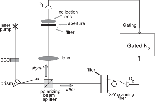
Figure 2: Schematic set-up of the first “ghost” image experiment. The experimental demonstrations of ghost imaging and ghost interference [4] in 1995 together stimulated the foundation of quantum imaging in terms of geometrical and physical optics.

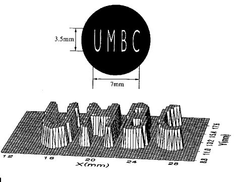
Figure 3: Upper: A reproduction of the actual aperture “UMBC” placed in the signal beam. Lower: The image of “UMBC”: coincidence counts as a function of the fiber tip’s transverse coordinates in the image plane. The step size is 0.25mm. The image shown is a “slice” at the half maximum value.

The first type-one ghost imaging experiment was demonstrated by Pittman et al. in 1995 [1] enlightened by the theoretical work of Klyshko [2]. The schematic setup of the experiment is shown in Fig. 2. A continuous wave (CW) laser is used to pump a nonlinear crystal to produce an entangled pair of orthogonally polarized signal (e-ray of the crystal) and idler (o-ray of the crystal) photons in the nonlinear optical process of spontaneous parametric down-conversion (SPDC). The pair emerges from the crystal collinearly with $\omega_{s}\cong\omega_{i}\cong\omega_{p}/2$ (degenerate SPDC). The pump is then separated from the signal-idler pair by a dispersion prism, and the signal and idler are sent in different directions by a polarization beam splitting Thompson prism. The signal photon passes through a convex lens of 400mm focal length and illuminates a chosen aperture (mask). As an example, one of the demonstrations used the letters “UMBC” for the object mask. Behind the aperture is the “bucket” detector package $D_{1}$, which is made by an avalanche photodiode placed at the focus of a short focal length collection lens. During the experiment $D_{1}$ is kept in a fixed position. The idler photon is captured by detector package $D_{2}$, which consists of an optical fiber coupled to another avalanche photodiode. The input tip of the fiber is scannable in the transverse plane by two step motors (along orthogonal directions). The output pulses of $D_{1}$ and $D_{2}$, both operate in the photon counting mode, are independently counted as the counting rate of $D_{1}$ and $D_{2}$, respectively, and simultaneously, sent to a coincidence circuit for counting the joint-detection events of the pair. The single detector counting rates of $D_{1}$ and $D_{2}$ are both monitored to be constants during the measurement. Surprisingly, a ghost image of the chosen aperture is observed in coincidences during the scanning of the fiber tip, when the following two experimental conditions are satisfactory: (1) $D_{1}$ and $D_{2}$ always measure a pair; (2) the distances $s_{o}$, which is the optical distance between the aperture to the lens, $s_{i}$, which is the optical distance from the imaging lens going backward along the signal photon path to the two-photon source of SPDC then going forward along the idler photon path to the fiber tip, and the focal length of the imaging lens $f$ satisfy the Gaussian thin lens equation of Eq. (1).

Figure 3 shows a typical measured ghost image. It is interesting to note that while the size of the “UMBC” aperture inserted in the signal path is only about 3.5mm$\times$7mm, the observed image measures 7mm$\times$14mm. The image is therefore magnified by a factor of 2 which equals the expected magnification $m=s_{i}/s_{o}$. In this measurement $s_{o}=$ 600mm and $s_{i}=$ 1200mm. When $D_{2}$ was scanned on transverse planes other than the ghost image plane the images blurred out.

The experiment was immediately given the name “ghost imaging” by the physics community due to its nonlocal feature. In the language of Einstein-Podolsky-Rosen (EPR) [3], the non-factorizable point-to-point image-forming correlation

$$G^{(2)}(\vec{\rho}_{o},\vec{\rho}_{i})\sim\delta(\vec{\rho}_{o}+\vec{\rho}_{i}/m)$$ (5)

observed in this experiment represents a nonlocal behavior of a measured pair of photons: neither the signal photon nor idler photon “knows” precisely where to go when the pair is created at the source. However, if one of them is observed at a point on the object plane, the other one must arrive at a unique corresponding point on the image plane. Although questions regarding fundamental issues of quantum theory still exist, the experimental demonstration of ghost imaging [1] and ghost interference [4] in 1995 together stimulated the foundation of quantum imaging in terms of geometrical and physical optics.

Type-two ghost imaging uses chaotic radiation sources. Different from type-one, the non-factorizable point-to-point image-forming correlation between the object and image planes is only partial with at least 50% constant background,

$$G^{(2)}(\vec{\rho}_{o},\vec{\rho}_{i})\sim 1+\delta(\vec{\rho}_{o}-\vec{\rho}_{i}).$$ (6)

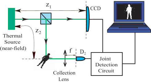
Figure 4: Near-field lensless ghost imaging of chaotic light demonstrated by Meyers et al.. $D_{2}$ is a “bucket” photon counting detector that is used to collect and count all random scattered and reflected photons from the object. The joint-detection between $D_{2}$ and the CCD array is realized by a photon-counting-coincidence circuit. $D_{2}$ is fixed in space. The counting rate of $D_{2}$ and the un-gated output of the CCD are both monitored to be constants during the measurement. Surprisingly, a 1:1 ghost image of the object is captured in joint-detection between $D_{2}$ and the CCD, when taking $z_{1}=z_{2}$. The images “blurred out” when the CCD is moved away from $z_{1}=z_{2}$, either in the direction of $z_{1}>z_{2}$ or $z_{1}<z_{2}$.

Figure 5: Ghost image of a toy soldier model.

The first near-field lensless ghost imaging experiment was demonstrated by Scarcelli et al in 2005 and 2006 [5][6] after their experimental demonstration of two-photon interference of chaotic light in 2004 [7]. Figure 4 illustrates an improved setup of the type-two ghost imaging experiment by Meyers et al. [8]. The thermal radiation of a chaotic source, which has a fairly large size in the transverse dimension, is split into two by a $50\%-50\%$ beamsplitter. One of the beams illuminates a toy soldier as shown in Fig. 4. The scattered and reflected photons from the solider (object) are collected and counted by a “bucket” detector $D_{2}$. In the other beam a high resolution CCD array, operating at the photon counting regime, is placed toward the radiation source for joint-detection with the “bucket” detector $D_{2}$. The counting rate of $D_{2}$ and the un-gated output of the CCD are both monitored to be constants during the measurement. Surprisingly, a 1:1 ghost image of the toy soldier is captured in the joint-detection between $D_{2}$ and the CCD, when taking $z_{1}=z_{2}$. The 1:1 ghost image of the toy soldier is shown in Fig. 5. The images “blurred out” when the CCD is moved away from $z_{1}=z_{2}$, either to the side of $z_{1}>z_{2}$ or $z_{1}<z_{2}$.

There is no doubt that chaotic radiations propagate to any transverse plane in a random and chaotic manner. A brief discussion for Fresnel free-propagation is given in the appendix. In the lensless ghost imaging experiment, a large transverse sized chaotic light source, as shown in Fig. 4, is usually used for achieving better spatial resolution. The source consists a large number of independent point sub-sources randomly distributed on the source plane. Each point sub-source may randomly radiate independent spherical waves to the object and image planes. Due to the chaotic nature of the source there is no interference between these sub-fields. These independent sub-intensities simply add together, yielding a constant total intensity in space and in time on any transverse plane. In the lensless ghost imaging setup, there is no lens applied to force these spherical waves collapsing to a point or a “speckle”, and there is no chance to have two identical copies of any “speckle” of the source onto the object and image planes. What is the physical cause of the point-to-point image-forming correlation? Although the non-factorizable point-to-point correlation between the object and image planes is only partial, the type-two ghost imaging looks more surprising than type-one because of the nature of the light source. Unlike the signal-idler photon pair, the jointly measured photons in type-two ghost imaging are just two independent photons that fall into the coincidence time window by chance only. Nevertheless, analogous to EPR, the non-factorizable partial point-to-point correlation represents a nonlocal behavior of a measured pair of independent photons: neither photon-one nor photon-two “knows” precisely where to go when they are created at each independent sub-sources; however, if one of them is observed at a point on the object plane, the other one has twice greater probability of arriving at a unique corresponding point on the image plane.

We have concluded and will show that the partial point-to-point correlation between the object and image planes in type-two ghost imaging is the result of two-photon interference. Similar to that of type-one, it involves the nonlocal superposition of two-photon amplitudes, a nonclassical entity corresponding to different yet indistinguishable alternative ways of triggering a joint-detection event [9]. Different from that of type-one, the joint-detection events observed in type-two ghost imaging are triggered by two randomly distributed independent photons. It is interesting to see that the quantum mechanical concept of two-photon interference is applicable to “classical” thermal light. In fact, this is not the first time in the history of physics we apply quantum mechanical concepts to thermal light. We should not forget Planck’s theory of blackbody radiation originated the quantum physics. The radiation Planck dealt with was thermal radiation. Although the concept of “two-photon interference” comes from the study of entangled biphoton states [9], the concept should not be restricted to entangled systems. The concept is generally true and applicable to any radiation, including “classical” thermal light. The partial point-to-point correlation of thermal radiation is not a new discovery either. The first set of temporal and spatial far-field intensity-intensity correlations of thermal light was demonstrated by Hanbury Brown and Twiss (HBT) in 1956 [10][11]. The HBT experiment created quite a surprise in the physics community and lead to a debate about the classical or quantum nature of the phenomenon [11][12]. Although the discovery of HBT initiated a number of key concepts of modern quantum optics, the HBT phenomenon itself was finally interpreted as statistical correlation of intensity fluctuations and considered as a classical effect. It is then reasonable to ask: Is the near-field type-two ghost imaging with thermal light a simple classical effect similar to that of HBT? Is it possible that the ghost imaging phenomenon itself, including the type-one ghost imaging of 1995, is merely a simple classical effect of intensity fluctuation correlation?[13][14][15][16] This article will address these important questions and explore the multi-photon interference nature of ghost imaging.

To explore the two-photon interference nature, we will analyze the physics of type-one and type-two ghost imaging in five steps. (1) Review the physics of coherent and incoherent light propagation; (2) Review classical imaging as the result of constructive-destructive interference among electromagnetic waves; (3) analyze type-one ghost imaging in terms of constructive-destructive interference between the biphoton amplitudes of an entangled photon-pair; (4) analyze type-two ghost imaging in terms of two-photon interference between chaotic sub-fields; and (5) discuss the physics of the phenomenon: whether it is a quantum interference or a classical intensity fluctuation correlation.

2 Classical Imaging

To understand the multi-photon interference nature of ghost imaging, it might be helpful to see the constructive-destructive interference nature of classical imaging first. We start from a typical classical imaging setup of Fig. 6 and ask a simple question: how does the radiation field propagate from the object plane to the image plane? In classical optics such propagation is usually described by an optical transfer function $h(\mathbf{r}-\mathbf{r}_{0},t-t_{0})$. We prefer to work with the single-mode propagator, namely the Green’s function, $g(\mathbf{k},\mathbf{r}-\mathbf{r}_{0},t-t_{0})$ [17][18], which propagates each mode of the radiation from space-time point ($\mathbf{r}_{0},t_{0}$) to space-time point ($\mathbf{r},t$). We treat the field $E(\mathbf{r},t)$ as a superposition of these modes. A detailed discussion about $g(\mathbf{k},\mathbf{r}-\mathbf{r}_{0},t-t_{0})$ is given in the Appendix. It is convenient to write the field $E(\mathbf{r},t)$ as a superposition of its longitudinal and transverse modes under the Fresnel paraxial approximation,

$$E(\vec{\rho},z,t)=\int d\vec{\kappa}\,d\omega\,\tilde{E}(\vec{\kappa},\omega)\,g(\vec{\kappa},\omega;\vec{\rho},z)\,e^{-i\omega t},$$ (7)

where $\tilde{E}(\vec{\kappa},\omega)$ is the complex amplitude for the mode of frequency $\omega$ and transverse wave-vector $\vec{\kappa}$. In Eq. (7) we have taken $z_{0}=0$ and $t_{0}=0$ at the object plane as usual. To simplify the notation, we have assumed one polarization.

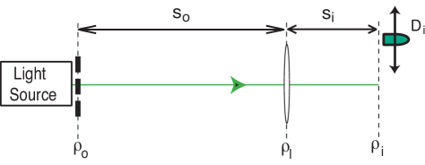
Figure 6: Typical imaging setup. A lens of finite size is used to produce a magnified or demagnified image of an object with limited spatial resolution.

Based on the experimental setup of Fig. 6 and following the Appendix, $g(\vec{\kappa},\omega;\vec{\rho},z)$ is found to be

$$\ \ \ \ g(\vec{\kappa},\omega;\vec{\rho}_{i},s_{o}+s_{i})$$

$$=\int_{obj}d\vec{\rho}_{o}\int_{lens}d\vec{\rho}_{l}\,\Big{\{}A(\vec{\rho}_{o})\,e^{i\vec{\kappa}\cdot\vec{\rho}_{o}}\Big{\}}\,\Big{\{}\frac{-i\omega}{2\pi c}\,\frac{e^{i\frac{\omega}{c}s_{o}}}{s_{o}}\,e^{i\frac{\omega}{2cs_{o}}|\vec{\rho}_{l}-\vec{\rho}_{o}|^{2}}\Big{\}}\,\,\Big{\{}e^{-i\frac{\omega}{2cf}\,|\vec{\rho}_{l}|^{2}}\Big{\}}\,$$

$$\ \ \ \ \times\,\Big{\{}\frac{-i\omega}{2\pi c}\,\frac{e^{i\frac{\omega}{c}s_{i}}}{s_{i}}\,e^{i\frac{\omega}{2cs_{i}}|\vec{\rho}_{i}-\vec{\rho}_{l}|^{2}}\Big{\}},$$ (8)

where $\vec{\rho}_{o}$, $\vec{\rho}_{l}$, and $\vec{\rho}_{i}$ are two-dimensional vectors defined, respectively, on the object, lens, and image planes. The first curly bracket includes the aperture function $A(\vec{\rho}_{o})$ of the object and the phase factor $e^{i\vec{\kappa}\cdot\vec{\rho}_{o}}$ contributed at the object plane by each transverse mode $\vec{\kappa}$. The terms in the second and fourth curly brackets describe free-space Fresnel propagation-diffraction from the source/object plane to the imaging lens, and from the imaging lens to the detection plane, respectively. The Fresnel propagator includes a spherical wave function $e^{i\frac{\omega}{c}(z_{j}-z_{k})}/(z_{j}-z_{k})$ and a Fresnel phase factor $e^{i\omega|\vec{\rho}_{j}-\vec{\rho}_{k}|^{2}/{2c(z_{j}-z_{k})}}$. The third curly bracket adds the phase factor introduced by the imaging lens.

We now rewrite Eq. (2) into the following form

$$g(\vec{\kappa},\omega;\vec{\rho}_{i},z=s_{o}+s_{i}) =\frac{-\omega^{2}}{(2\pi c)^{2}s_{o}s_{i}}\,e^{i\frac{\omega}{c}(s_{o}+s_{i})}\,e^{i\frac{\omega}{2cs_{i}}|\vec{\rho}_{i}|^{2}}\int_{obj}d\vec{\rho}_{o}\,A(\vec{\rho}_{o})\,e^{i\frac{\omega}{2cs_{o}}|\vec{\rho}_{o}|^{2}}\,e^{i\vec{\kappa}\cdot\vec{\rho}_{o}}$$

$$\ \ \ \ \times\int_{lens}d\vec{\rho}_{l}\,e^{i\frac{\omega}{2c}[\frac{1}{s_{o}}+\frac{1}{s_{i}}-\frac{1}{f}]|\vec{\rho}_{l}|^{2}}\,e^{-i\frac{\omega}{c}(\frac{\vec{\rho}_{o}}{s_{o}}+\frac{\vec{\rho}_{i}}{s_{i}})\cdot\vec{\rho}_{l}}.$$ (9)

The image plane is defined by the Gaussian thin-lens equation of Eq. (1). Hence, the second integral in Eq. (2) reduces to, for a finite sized lens of radius $R$, the so-called point-spread function, or the Airy disk, of the imaging system:

$$\int_{lens}d\vec{\rho}_{l}\,e^{-i\frac{\omega}{c}(\frac{\vec{\rho}_{o}}{s_{o}}+\frac{\vec{\rho}_{i}}{s_{i}})\cdot\vec{\rho}_{l}}=\frac{2J_{1}(x)}{x}=somb(x),$$ (10)

where the sombrero-like function $somb(x)=2J_{1}(x)/x$ with argument $x=[\frac{R}{s_{o}}\,\frac{\omega}{c}|\vec{\rho}_{o}+\rho_{i}/m|]$ has been defined in Eq. (3). Eq. (10) indicates a constructive interference.

Substituting Eqs. (2) and (10) into Eq. (7) enables one to obtain the classical self-correlation function of the field, or, equivalently, the intensity on the image plane

$$I(\vec{\rho}_{i},z_{i},t_{i})=\langle\,E^{*}(\vec{\rho}_{i},z_{i},t_{i})\,E(\vec{\rho}_{i},z_{i},t_{i})\,\rangle,$$ (11)

where $\langle...\rangle$ denotes an ensemble average. To simplify the mathematics, monochromatic light is assumed as usual.

Case (I): Incoherent imaging. The ensemble average yields zeros except when $\vec{\kappa}=\vec{\kappa^{\prime}}$. The image is thus

$$I(\vec{\rho}_{i}) \propto \int d\vec{\rho}_{o}\,\big{|}A(\vec{\rho}_{o})\big{|}^{2}\,somb^{2}[\frac{R}{s_{o}}\,\frac{\omega}{c}|\vec{\rho}_{o}+\frac{\vec{\rho}_{i}}{m}|].$$ (12)

An incoherent image, magnified by a factor of $m$, is thus given by the convolution between the modulus square of the object aperture function and the point-spread function. The spatial resolution of the image is determined by the finite width of the $|somb|^{2}$-function.

Case (II): Coherent imaging. The coherent superposition of the $\vec{\kappa}$ modes in both $E^{*}(\vec{\rho}_{i},\tau)$ and $E(\vec{\rho}_{i},\tau)$ results in a wavepacket. The image, or the intensity distribution on the image plane, is

$$I(\vec{\rho}_{i})\propto\Big{|}\int_{obj}d\vec{\rho}_{o}\,A(\vec{\rho}_{o})\,e^{i\frac{\omega}{2cs_{o}}|\vec{\rho}_{o}|^{2}}somb[\frac{R}{s_{o}}\frac{\omega}{c}|\vec{\rho}_{o}+\frac{\vec{\rho}_{i}}{m}|]\Big{|}^{2}.$$ (13)

A coherent image, magnified by a factor of $m$, is thus given by the modulus square of the convolution between the object aperture function (multiplied by a Fresnel phase factor) and the point-spread function.

For $s_{i}<s_{o}$ and $s_{o}>f$, both Eqs. (12) and (13) describe a real demagnified inverted image. In both cases, a narrower $somb$-function yields a higher spatial resolution. Therefore the use of a larger imaging lens and shorter wavelengths will improve the spatial resolution of an imaging system.

3 Biphoton and type-one ghost imaging

In this section we analyze type-one ghost imaging. Type-one ghost imaging uses entangled photon pairs such as the signal-idler biphoton pairs of SPDC [19][9]. The nearly collinear signal-idler system generated by SPDC can be described, in the ideal case, by the following entangled biphoton state [9]:

$$|\,\Psi\,\rangle=\Psi_{0}\int d\vec{\kappa}_{s}\,d\vec{\kappa}_{i}\,\delta(\vec{\kappa}_{s}+\vec{\kappa}_{i})\int d\omega_{s}\,d\omega_{i}\,\delta(\omega_{s}+\omega_{i}-\omega_{p})\,a^{{\dagger}}(\vec{\kappa}_{s},\omega_{s})\,a^{{\dagger}}(\vec{\kappa}_{i},\omega_{i})\,|\,0\,\rangle,$$ (14)

where $\omega_{j}$, $\vec{\kappa}_{j}$ ($j=s,i,p$), are the frequency and transverse wavevector of the signal, idler, and pump, respectively. For simplicity a CW single mode pump with $\vec{\kappa}_{p}=0$ is assumed. Eq. (14) indicates that the biphoton state of the signal-idler pair is an entangled state. The single-photon state of the signal and the idler can be evaluated by taking a partial trace of its twin,

$$\hat{\rho}_{s} =tr_{i}\,|\,\Psi\,\rangle\langle\,\Psi\,|=\int d\vec{\kappa}_{s}\,d\omega_{s}\,a^{{\dagger}}(\vec{\kappa}_{s},\omega_{s})|\,0\,\rangle\langle\,0\,|a(\vec{\kappa}_{s},\omega_{s}),$$

$$\hat{\rho}_{i} =tr_{s}\,|\,\Psi\,\rangle\langle\,\Psi\,|=\int d\vec{\kappa}_{i}\,d\omega_{i}\ a^{{\dagger}}(\vec{\kappa}_{i},\omega_{i})|\,0\,\rangle\langle\,0\,|a(\vec{\kappa}_{i},\omega_{i}).$$ (15)

Although the signal-idler system is in a pure state, the state of the signal photon and the idler photon, respectively, are both mixed states.

Let us imagine a measurement in which two point-like photon counting detectors ($D_{1}$ and $D_{2}$) are placed at the output plane of an SPDC source for the detection of the signal photon and the idler photon, respectively, and for the joint-detection of the signal-idler pair. The probability of observing a photo-detection event in the SPDC output plane $\vec{\rho}_{j}$ at time $t_{j}$, $j=s,i$, is calculated from the first-order photo-detection theory of Glauber [20]

$$G^{(1)}(\vec{\rho}_{j},t_{j})=tr\,\hat{\rho}\,E^{(-)}(\vec{\rho}_{j},t_{j})E^{(+)}(\vec{\rho}_{j},t_{j}),$$ (16)

where we have chosen $z_{j}=0$ for the SPDC output plane as usual. It is easy to find that

$$G^{(1)}(\vec{\rho}_{s},t_{s})=\text{constant},\ \ \ \ G^{(1)}(\vec{\rho}_{i},t_{i})=\text{constant},$$ (17)

which means that the signal photon and the idler photon both have equal probability to be observed at any position in the output plane of the SPDC at any time. The probability of observing a joint-detection event between $D_{1}$ and $D_{2}$ located at $\vec{\rho}_{s}$ and $\vec{\rho}_{i}$ in the SPDC output plane of $z_{s}=z_{i}=0$ is calculated from the second-order photo-detection theory of Glauber [20]:

$$\hskip 14.22636ptG^{(2)}(\vec{\rho}_{s},t_{s};\vec{\rho}_{i},t_{i})$$

$$=\langle\,\Psi\,|\,E^{(-)}_{s}(\vec{\rho}_{s},t_{s})E^{(-)}_{i}(\vec{\rho}_{i},t_{i})E^{(+)}_{i}(\vec{\rho}_{i},t_{i})E^{(+)}_{s}(\vec{\rho}_{s},t_{s})\,|\,\Psi\,\rangle$$

$$=|\langle\,0\,|\,E^{(+)}_{i}(\vec{\rho}_{i},t_{i})E^{(+)}_{s}(\vec{\rho}_{s},t_{s})\,|\,\Psi\,\rangle|^{2}$$

$$\equiv|\,\Psi(\vec{\rho}_{s},t_{s};\vec{\rho}_{i},t_{i})\,|^{2},$$ (18)

where $\Psi(\vec{\rho}_{s},t_{s};\vec{\rho}_{i},t_{i})$ is defined as the effective biphoton wavefunction. The transverse spatial part of the effective biphoton wavefunction is easily calculated to be:

$$\Psi(\vec{\rho}_{s},\vec{\rho}_{i})\simeq\delta(\vec{\rho}_{s}-\vec{\rho}_{i}),$$ (19)

under the condition $t_{s}\simeq t_{i}$. Equations (14), (17), and (19) suggest that the entangled signal-idler photon pair is characterized by the EPR correlation [3] in transverse momentum and transverse position; hence, similar to the original EPR state, we have [21]:

$$\Delta(\vec{\kappa}_{s}+\vec{\kappa}_{i})=0\,\,\,\,\&\,\,\,\Delta(\vec{\rho}_{s}-\vec{\rho}_{i})=0\,\,$$

with $$\Delta\vec{\kappa}_{s}\sim\infty,\hskip 5.69054pt\Delta\vec{\kappa}_{i}\sim\infty,\hskip 5.69054pt\Delta\vec{\rho}_{s}\sim\infty,\hskip 5.69054pt\Delta\vec{\rho}_{i}\sim\infty.$$

In EPR’s language, the signal photon and the idler photon may come from any point in the output plane of the SPDC. However, if the signal (idler) is found in a certain position, the idler (signal) must be observed in the same position, with certainty (100%). Simultaneously, the signal photon and the idler photon may have any transverse momentum. However, if a certain value and direction of the transverse momentum of the signal (idler) is observed, the transverse momentum of the idler (signal) will be uniquely determined with equal value and opposite direction.

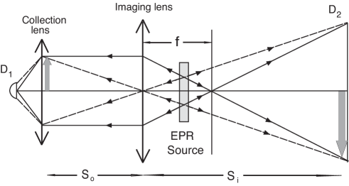
Figure 7: An unfolded schematic of the 1995 ghost imaging experiment, which is helpful for understanding the physics. Since the biphoton “light” propagates along “straight lines”, it is obvious that any point on the object plane corresponds to a unique point on the image plane. Although the placement of the lens, the object, and detector $D_{2}$ obeys the Gaussian thin lens equation, it is important to notice that the geometric rays in the figure actually represent the biphoton amplitudes of an entangled photon pair. The point-to-point correspondence is the result of a constructive-destructive interference of these biphoton amplitudes.

The EPR $\delta$-functions, $\delta(\vec{\rho}_{s}-\vec{\rho}_{i})$ and $\delta(\vec{\kappa}_{s}+\vec{\kappa}_{i})$ in transverse position and momentum, are the key to understanding the ghost imaging experiment of Pittman et al. of 1995. $\delta(\vec{\rho}_{s}-\vec{\rho}_{i})$ indicates that the signal-idler pair is always emitted from the same point on the output plane of the biphoton source. Simultaneously, $\delta(\vec{\kappa}_{s}+\vec{\kappa}_{i})$ defines the angular correlation of the pair: the signal-idler pair always exists at roughly equal but opposite angles relative to the pump for degenerate SPDC. This then allows for a simple explanation of the experiment in terms of “usual” geometrical optics in the following manner: we envision the nonlinear crystal as a “hinge point” and “unfold” the schematic of Fig. 2 into the Klyshko picture [2] of Fig. 7. The signal-idler biphoton amplitudes can then be represented by straight lines (but keep in mind the different propagation directions) and therefore the image is reproduced in coincidences when the aperture, lens, and fiber tip are located according to the Gaussian thin lens equation of Eq. (1). The image is exactly the same as that one would observe on a screen placed at the fiber tip if detector $D_{1}$ were replaced by a point-like light source and the nonlinear crystal by a reflecting mirror.

Comparing the “unfolded” schematic of the ghost imaging experiment with that of the classical imaging setup of Fig. 1, it is not difficult to find that any “light point” on the object plane has a unique corresponding “light point” on the image plane. This point-to-point correspondence is the result of the constructive-destructive interference among these biphoton amplitudes that are illustrated as the geometrical rays in Fig. 7. Similar to the situation in classical imaging, these biphoton amplitudes which experience equal optical path propagation will superpose constructively at each pair of one-to-one points of the object plane and the image plane for a joint-detection event, while these that experience unequal distance propagation will superpose destructively at all other points on the object and image planes. The use of the imaging lens makes this constructive-destructive interference possible. It is this unique point-to-point EPR correlation that makes the “ghost” image of the object-aperture function possible. Despite the completely different physics from classical optics, the remarkable feature is that the relationship between the focal length $f$ of the lens, the aperture’s optical distance $s_{o}$, and the image’s optical distance $s_{i}$, satisfies the Gaussian thin lens equation of Eq. (1). It is worth emphasizing again that the geometric rays in Fig. 7 represent the biphoton amplitudes of a signal-idler photon pair, and the point-to-point correspondence is the result of the constructive-destructive interference of these biphoton amplitudes.

We now calculate $G^{(2)}(\vec{\rho}_{1},\vec{\rho}_{2})$ for the “ghost” imaging experiment in detail, where $\vec{\rho}_{1}$ and $\vec{\rho}_{2}$ are the transverse coordinates of the point-like photodetector $D_{1}$ and $D_{2}$, on the object and image planes, respectively. We will show that there exists a $\delta$-function-like point-to-point correlation between the object and image planes, $\delta(\vec{\rho}_{1}-\vec{\rho}_{2}/m)$. We will then show how the object function of $A(\vec{\rho}_{o})$ is transferred to the image plane as a magnified image $A(\vec{\rho}_{2}/m)$.

We first calculate the effective biphoton wavefunction $\Psi(\vec{\rho}_{1},z_{1},t_{1};\vec{\rho}_{2},z_{2},t_{2})$, as defined in Eq. (3). By inserting the field operators into $\Psi(\vec{\rho}_{1},z_{1},t_{1};\vec{\rho}_{2},z_{2},t_{2})$, and considering the commutation relations of the field operators, the effective biphoton wavefunction is calculated to be

$$\Psi(\vec{\rho}_{1},z_{1},t_{1};\vec{\rho}_{2},z_{2},t_{2}) =\Psi_{0}\int d\vec{\kappa}_{s}\,d\vec{\kappa}_{i}\,\delta(\vec{\kappa}_{s}+\vec{\kappa}_{i})\int d\omega_{s}\,d\omega_{i}\,\delta(\omega_{s}+\omega_{i}-\omega_{p})$$ (21)

$$\hskip 14.22636pt\times\,g(\vec{\kappa}_{s},\omega_{s};\vec{\rho}_{1},z_{1})\,e^{-i\omega_{s}t_{1}}\,g(\vec{\kappa}_{i},\omega_{i};\vec{\rho}_{2},z_{2})\,e^{-i\omega_{i}t_{2}}.$$

Equation (21) indicates a coherent superposition of all the biphoton amplitudes shown in Fig. 7. Next, we follow the unfolded experimental setup of Fig. 8 to establish the Green’s functions $g(\vec{\kappa}_{s},\omega_{s},\vec{\rho}_{1},z_{1})$ and $g(\vec{\kappa}_{i},\omega_{i},\vec{\rho}_{2},z_{2})$. In arm-$1$ the signal propagates freely over a distance $d_{1}$ from the output plane of the source to the imaging lens, passes an object aperture at distance $s_{o}$, and then is focused onto photon-counting detector $D_{1}$ by a collection lens. We will evaluate $g(\vec{\kappa}_{s},\omega_{s},\vec{\rho}_{1},z_{1})$ by propagating the field from the output plane of the biphoton source to the object plane. In arm-$2$ the idler propagates freely over a distance $d_{2}$ from the output plane of the biphoton source to a point-like detector $D_{2}$. $g(\vec{\kappa}_{i},\omega_{i},\vec{\rho}_{2},z_{2})$ is thus a free propagator.

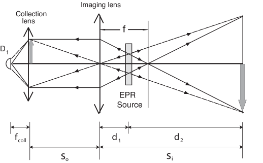
Figure 8: In arm-$1$ the signal propagates freely over a distance $d_{1}$ from the output plane of the source to the imaging lens, passes an object aperture at distance $s_{o}$, and then is focused onto photon-counting detector $D_{1}$ by a collection lens. In arm-$2$ the idler propagates freely over a distance $d_{2}$ from the output plane of the source to a point-like photon counting detector $D_{2}$.

(I) Arm-$1$ (source to object):

The optical transfer function or Green’s function in arm-$1$, which propagates the field from the source plane to the object plane, is given by:

$$g(\vec{\kappa}_{s},\omega_{s};\vec{\rho}_{1},z_{1}=d_{1}+s_{o}) =e^{i\frac{\omega_{s}}{c}z_{1}}\int_{lens}d\vec{\rho}_{l}\,\int_{source}d\vec{\rho}_{s}\,\Big{\{}\,\frac{-i\omega_{s}}{2\pi cd_{1}}e^{i\vec{\kappa_{s}}\cdot\vec{\rho}_{s}}\,e^{i\frac{\omega_{s}}{2cd_{1}}|\,\vec{\rho}_{s}-\vec{\rho}_{l}\,|^{2}}\Big{\}}$$

$$\ \ \ \ \times\,e^{-i\frac{\omega}{2cf}\,|\vec{\rho}_{l}|^{2}}\,\Big{\{}\,\frac{-i\omega_{s}}{2\pi cs_{o}}\,e^{i\frac{\omega_{s}}{2cs_{o}}|\,\vec{\rho}_{l}-\vec{\rho}_{1}\,|^{2}}\Big{\}},$$ (22)

where $\vec{\rho}_{s}$ and $\vec{\rho}_{l}$ are the transverse vectors defined, respectively, on the output plane of the source and on the plane of the imaging lens. The terms in the first and second curly brackets in Eq. (3) describe free space propagation from the output plane of the source to the imaging lens and from the imaging lens to the object plane, respectively. Again, $e^{i\frac{\omega_{s}}{2cd_{1}}|\,\vec{\rho}_{s}-\vec{\rho}_{l}\,|^{2}}$ and $e^{i\frac{\omega_{s}}{2cs_{o}}|\,\vec{\rho}_{l}-\vec{\rho}_{1}\,|^{2}}$ are the Fresnel phases as defined in the Appendix. Here the imaging lens is treated as a thin-lens, and the transformation function of the imaging lens is approximated as a Gaussian, $l(|\vec{\rho}_{l}|,f)\cong e^{-i\frac{\omega}{2cf}\,|\vec{\rho}_{l}|^{2}}$.

(II) Arm-$2$ (from source to image):

In arm-$2$, the idler propagates freely from the source to the plane of $D_{2}$, which is also the plane of the image. The Green’s function is

$$g(\vec{\kappa}_{i},\omega_{i};\vec{\rho}_{2},z_{2}=d_{2})=\frac{-i\omega_{i}}{2\pi cd_{2}}\,e^{i\frac{\omega_{i}}{c}d_{2}}\int_{source}d\vec{\rho^{\prime}_{s}}\,e^{i\frac{\omega_{i}}{2cd_{2}}|\,\vec{\rho^{\prime}_{s}}-\vec{\rho}_{2}\,|^{2}}\,e^{i\vec{\kappa}_{i}\cdot\vec{\rho^{\prime}_{s}}}$$ (23)

where $\vec{\rho^{\prime}_{s}}$ and $\vec{\rho}_{2}$ are the transverse vectors defined, respectively, on the output plane of the source and the plane of photodetector $D_{2}$.

(III) $\Psi(\vec{\rho}_{1},\vec{\rho}_{2})$ and $G^{(2)}(\vec{\rho}_{1},\vec{\rho}_{2})$ (object plane - image plane):

For simplicity, in the following calculation we consider degenerate ($\omega_{s}=\omega_{i}=\omega$) and collinear SPDC. The effective transverse biphoton wavefunction $\Psi(\vec{\rho}_{1},\vec{\rho}_{2})$ is then evaluated by substituting the Green’s functions $g(\vec{\kappa}_{s},\omega;\vec{\rho}_{1},z_{1})$ and $g(\vec{\kappa}_{i},\omega;\vec{\rho}_{2},z_{2})$ into Eq. (21),

$$\Psi(\vec{\rho}_{1},\vec{\rho}_{2}) \propto\int d\vec{\kappa}_{s}\,d\vec{\kappa}_{i}\,\delta(\vec{\kappa}_{s}+\vec{\kappa}_{i})\,g(\vec{\kappa}_{s},\omega;\vec{\rho}_{1},z_{1})\,g(\vec{\kappa}_{i},\omega;\vec{\rho}_{2},z_{2})$$

$$\propto e^{i\frac{\omega}{c}(s_{o}+s_{i})}\int d\vec{\kappa}_{s}\,d\vec{\kappa}_{i}\,\delta(\vec{\kappa}_{s}+\vec{\kappa}_{i})\int_{lens}d\vec{\rho}_{l}\,\int_{source}d\vec{\rho}_{s}\,\,e^{i\vec{\kappa_{s}}\cdot\vec{\rho}_{s}}e^{i\frac{\omega}{2cd_{1}}|\,\vec{\rho}_{s}-\vec{\rho}_{l}\,|^{2}}$$

$$\ \ \ \ \times\,e^{-i\frac{\omega}{2cf}\,|\vec{\rho}_{l}|^{2}}\,\,e^{i\frac{\omega_{s}}{2cs_{o}}|\,\vec{\rho}_{l}-\vec{\rho}_{1}\,|^{2}}\int_{source}d\vec{\rho^{\prime}_{s}}\,\,e^{i\vec{\kappa}_{i}\cdot\vec{\rho^{\prime}_{s}}}\,e^{i\frac{\omega_{i}}{2cd_{2}}|\,\vec{\rho^{\prime}_{s}}-\vec{\rho}_{2}\,|^{2}}$$ (24)

where all the proportionality constants have been ignored. After completing the double integral of $d\vec{\kappa}_{s}$ and $d\vec{\kappa}_{i}$

$$\int d\vec{\kappa}_{s}\,d\vec{\kappa}_{i}\,\delta(\vec{\kappa}_{s}+\vec{\kappa}_{i})\,e^{i\vec{\kappa_{s}}\cdot\vec{\rho}_{s}}\,e^{i\vec{\kappa}_{i}\cdot\vec{\rho^{\prime}_{s}}}\sim\,\delta(\vec{\rho}_{s}-\vec{\rho^{\prime}_{s}}),$$

Eq. (3) becomes

$$\Psi(\vec{\rho}_{1},\vec{\rho}_{2})\propto e^{i\frac{\omega}{c}(s_{0}+s_{i})}\int_{lens}d\vec{\rho}_{l}\int_{source}d\vec{\rho}_{s}\,e^{i\frac{\omega}{2cd_{2}}|\,\vec{\rho}_{2}-\vec{\rho}_{s}\,|^{2}}\,e^{i\frac{\omega}{2cd_{1}}|\,\vec{\rho}_{s}-\vec{\rho}_{l}\,|^{2}}\,e^{-i\frac{\omega}{2cf}\,|\vec{\rho}_{l}|^{2}}\,e^{i\frac{\omega}{2cs_{o}}|\,\vec{\rho}_{l}-\vec{\rho}_{o}\,|^{2}}.$$

Next, we complete the integral for $d\vec{\rho}_{s}$,

$$\Psi(\vec{\rho}_{1},\vec{\rho}_{2})\propto e^{i\frac{\omega}{c}(s_{0}+s_{i})}\int_{lens}d\vec{\rho}_{l}\,e^{i\frac{\omega}{2cs_{i}}|\,\vec{\rho}_{2}-\vec{\rho}_{l}\,|^{2}}\,e^{-i\frac{\omega}{2cf}\,|\vec{\rho}_{l}|^{2}}e^{i\frac{\omega}{2cs_{o}}|\,\vec{\rho}_{l}-\vec{\rho}_{1}\,|^{2}},$$ (25)

where we have replaced $d_{1}+d_{2}$ with $s_{i}$ (as depicted in Fig. 8). Although the signal and idler propagate in different directions along two optical arms, interestingly, the Green function in Eq. (25) is equivalent to that of a classical imaging setup, as if the field is originated from a point $\vec{\rho}_{1}$ on the object plane and propagated the lens and then arrived at point $\vec{\rho}_{2}$ on the imaging plane. The mathematics is consistent with our previous qualitative analysis of the experiment.

The finite integral on $d\vec{\rho}_{l}$ yields a point-to-“spot” relationship between the object plane and the image plane that is defined by the Gaussian thin-lens equation

$$\Psi(\vec{\rho}_{1},\vec{\rho}_{2})\propto\int_{lens}d\vec{\rho}_{l}\,e^{i\frac{\omega}{2c}[\frac{1}{s_{o}}+\frac{1}{s_{i}}-\frac{1}{f}]|\,\vec{\rho}_{l}|^{2}}\,e^{-i\frac{\omega}{c}(\frac{\vec{\rho}_{1}}{s_{o}}+\frac{\vec{\rho}_{2}}{s_{i}})\cdot\vec{\rho}_{l}}=somb\Big{(}\frac{R}{s_{o}}\,\frac{\omega}{c}|\vec{\rho}_{1}+\frac{\vec{\rho}_{2}}{m}|\Big{)}.$$ (26)

If the integral is taken to infinity, by imposing the condition of the Gaussian thin-lens equation the effective transverse biphoton wavefunction can be approximated as a $\delta$ function

$$\Psi(\vec{\rho}_{1},\vec{\rho}_{2})\sim\delta(\vec{\rho}_{1}+\vec{\rho}_{2}/m)\sim\delta(\vec{\rho}_{o}+\vec{\rho}_{I}/m),$$ (27)

where we have replaced $\vec{\rho}_{1}$ and $\vec{\rho}_{2}$ with $\vec{\rho}_{o}$ and $\vec{\rho}_{I}$, respectively, to emphasize the point-to-point EPR correlation between the object and image planes. To avoid confusion with the “idler” we have used $\vec{\rho}_{I}$ to label the image plane.

We now include an object-aperture function, a collection lens and a photon counting detector $D_{1}$ into the optical transfer function of arm-$1$ as shown in Fig. 2. The collection-lens$-D_{1}$ package can be simply treated as a “bucket” detector. The “bucket” detector integrates the biphoton amplitudes $\Psi(\vec{\rho}_{o},\vec{\rho}_{2})$, which are modulated by the object aperture function $A(\vec{\rho}_{o})$ into a joint photodetection event. This process is equivalent to the following convolution

$$R_{1,2}\propto\int_{object}d\vec{\rho}_{o}\,\big{|}A(\vec{\rho}_{o})\big{|}^{2}\,\big{|}\Psi(\vec{\rho}_{o},\vec{\rho}_{2})\big{|}^{2}\simeq\big{|}A(\vec{\rho}_{2}/m)\big{|}^{2}=\big{|}A(\vec{\rho}_{I}/m)\big{|}^{2}.$$ (28)

Again, $D_{2}$ is scanned in the image plane ($\vec{\rho}_{2}=\vec{\rho}_{I}$). A ghost image of the object is thus reproduced on the image plane by means of the joint-detection between the point-like-detector $D_{2}$ and the bucket detector $D_{1}$.

The physical process corresponding to the above convolution is rather simple. Suppose the point detector $D_{2}$ is triggered by an idler photon at a transverse position of $\vec{\rho}_{\textrm{I}}$ in a joint-detection event with the bucket detector $D_{1}$ which is triggered by the signal twin that is either transmitted or reflected from a unique point $\vec{\rho}_{\textrm{o}}$ on the object plane. This unique point-to-point determination comes from the non-factorizable correlation function $\delta(\vec{\rho}_{\textrm{o}}+\vec{\rho}_{I}/m)$. Now, we move $D_{2}$ to another transverse position $\vec{\rho^{\prime}}_{I}$ and register a joint-detection event. The signal photon that triggers $D_{1}$ must be either transmitted or reflected from another unique point $\vec{\rho^{\prime}}_{o}$ on the object plane which is determined by $\delta(\vec{\rho^{\prime}}_{\textrm{o}}+\vec{\rho^{\prime}}_{\textrm{I}}/m)$. The chances of receiving a joint detection event at $\vec{\rho}_{\textrm{I}}$ and at $\vec{\rho^{\prime}}_{\textrm{I}}$ would be modulated by the values of the aperture function $A(\vec{\rho}_{\textrm{o}})$ and $A(\vec{\rho^{\prime}}_{\textrm{o}})$, respectively. Accumulating a large number of joint-detection events at each transverse coordinates on the image plane, the aperture function $A(\vec{\rho}_{\textrm{o}})$ is thus reproduced in the joint-detection as a function of $\vec{\rho}_{\textrm{I}}$.

The observation of type-one ghost imaging has demonstrated a non-factorizable point-to-point EPR correlation between the object and image planes. This point-to-point correlation is the result of a constructive-destructive interference between biphoton amplitudes,

$$G^{(2)}(\vec{\rho}_{o},\vec{\rho}_{I})=\Big{|}\int d\vec{\kappa}_{s}\,d\vec{\kappa}_{i}\,\delta(\vec{\kappa}_{s}+\vec{\kappa}_{i})\,g(\vec{\kappa}_{s},\vec{\rho}_{o})\,g(\vec{\kappa}_{i},\vec{\rho}_{I})\Big{|}^{2}=somb^{2}\Big{(}\frac{R}{s_{o}}\,\frac{\omega}{c}|\vec{\rho}_{O}+\frac{\vec{\rho}_{I}}{m}|\Big{)}.$$ (29)

In this view we consider the ghost imaging experiment of Pittman et al. a realization of the 1935 EPR gedankenexperiment [21] [22].

Classical theory has difficulties when facing type-one ghost imaging phenomenon. In the classical theory of light, a joint measurement between two photodetectors $D_{1}$ and $D_{2}$ measures the statistical correlation of intensity fluctuations,

$$G^{(2)}(\vec{\rho}_{1},\vec{\rho}_{2})=\langle\,I(\vec{\rho}_{1})\,I(\vec{\rho}_{2})\,\rangle=\bar{I}(\vec{\rho}_{1})\bar{I}(\vec{\rho}_{2})+\langle\,\Delta I(\vec{\rho}_{1})\Delta I(\vec{\rho}_{2})\rangle.$$ (30)

Therefore, the point-to-point image-forming correlation is considered as a result of the statistical correlation of intensity fluctuations between the object and the image planes. Comparing Eq. (30), which has a constant background $\bar{I}(\vec{\rho}_{1})\bar{I}(\vec{\rho}_{2})$, with Eq. (29), which has a zero background, the mean intensities $\bar{I}(\vec{\rho}_{1})$ and $\bar{I}(\vec{\rho}_{2})$ must be zero, otherwise the result would lead to non-physical conclusions. The measurements, however, never yield zero mean values of $\bar{I}(\vec{\rho}_{1})$ and $\bar{I}(\vec{\rho}_{2})$ under any circumstances. In fact, the individual-detector counting rates of $D_{1}$ and $D_{2}$ were monitored in the experiment of Pittman et al. with much greater value than that of the coincidences. It is clear that the classical theory of statistical correlation of intensity fluctuations does not reflect the correct physics behind type-one ghost imaging.

4 Type-two ghost imaging with chaotic radiation

In this section we discuss the physics of type-two ghost imaging. The near-field lensless ghost imaging with chaotic radiation was first demonstrated by Scarcelli et al. in the years from 2005 to 2006 [5][6] following their experimental demonstration of two-photon interference of chaotic light [7].

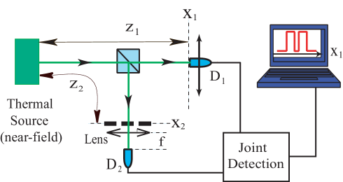
Figure 9: Near-field lensless ghost imaging with chaotic light demonstrated in 2006 by Scarcelli et al. $D_{1}$ is a point-like photodetector that is scannable along the $x_{1}$-axis. The joint-detection between $D_{1}$ and the bucket detector $D_{2}$ is realized either by a photon-counting coincidence counter or by a standard HBT linear multiplier (RF mixer). In this measurement $D_{2}$ is fixed in the focal point of a convex lens, playing the role of a bucket detector. The counting rate or the photocurrent of $D_{1}$ and $D_{2}$, respectively, are measured to be constants. Surprisingly, an image of the 1-D object is observed in the joint-detection between $D_{1}$ and $D_{2}$ by scanning $D_{1}$ in the plane of $z_{1}=z_{2}$ along the $x_{1}$-axis. The image, is blurred out when $z_{1}\neq z_{2}$. There is no doubt that thermal radiations propagate to any transverse plane in a random and chaotic manner. There is no lens applied to force the thermal radiation “collapsing” to a point or speckle either. What is the physical cause of the point-to-point image-forming correlation in coincidences?

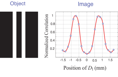
Figure 10: The double-slit and its ghost image. Notice, the constant background has been removed from the correlation.

The schematic experimental setup of their 2006 demonstration is shown in Fig. 9. Radiation with a narrow spectral bandwidth $\Delta\omega$ of a few millimeters diameter from a chaotic pseudothermal source [23] was equally divided into two by a $50\%-50\%$ non-polarizing beam-splitter. In the reflected arm, a double-slit with slit separation $b=1.5$ mm and slit width $a=0.2$ mm, was placed at a distance $z_{2}=139$ mm from the source and a bucket detector $D_{2}$ was placed just behind the object. In the transmitted arm a point detector $D_{1}$ was scanned in the transverse plane of $z_{1}=z_{2}$. Scarcelli et al tested two different joint detection schemes, namely the photon counting coincidence circuit and the standard HBT correlator. In the photon counting regime two Geiger mode avalanche photodiodes were employed for single-photon detection. In the bright light condition, two silicon PIN diodes were used with a standard analog HBT linear multiplier. The bucket detector $D_{2}$ was simulated by using a short focal length lens ($f=25mm$) to focus the light coming from the object onto the active area of the detector while the point detector $D_{2}$ was simulated by a pinhole like aperture. After a large number of reaped measurements for different experimental schemes and conditions, Scarcelli et al reported the following observations.

Observation (1): A typical measured ghost image of the double-slit is shown in Fig. 10. The measured curve reports the joint-detection counting rate between $D_{1}$ and $D_{2}$, or the output current of a HBT linear multiplier, as a function of the transverse position of the point detector $D_{1}$ along $x_{1}$ axis. Notice, in Fig. 10 the constant background has been removed from the correlation.

Observation (2): The measured contrasts vary significantly under different experimental schemes and conditions. It was found that the image contrast can achieve $\sim 50\%$ in photon counting measurement if no more than one joint-detection event occurring within the time window of the coincidence circuit. $50\%$ is the maximum image contrast we expect for thermal light ghost imaging.

Observation (3): To achieve less than one joint-detection event per coincidence time window, weak light source is not a necessary condition. It can be easily achieved under bright light condition by using adjustable ND-filters with $D_{1}$ and $D_{2}$.

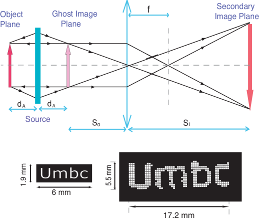
Figure 11: Unfolded schematic experimental setup of a secondary image measurement of the ghost image and the measured secondary images. By using a convex lens of focal length $f$, the ghost image is imaged onto a secondary image plane, which is defined by the Gaussian thin-lens equation, $1/s_{o}+1/s_{i}=1/f$, with magnification $m=-s_{i}/s_{o}$. This setup is useful for distant large scale ghost imaging applications.

To confirm the observations are imaged images, and not “projection shadows”, Scarcelli et al. made two additional measurements. In the first measurement, photodetector $D_{1}$ was moved away from the ghost image plane of $z_{1}=z_{2}$. Whether moved in the direction of $z_{1}>z_{2}$ or $z_{1}<z_{2}$, the ghost image became “blurred”. The measurement also showed that the depth of the image is a function of the angular size of the thermal source: a larger angular sized source (opening angle $\Delta\theta$ relative to the photodetectors) produces sharper image with shorter image depth. In the second measurement, Scarcelli et al. constructed a secondary imaging system, illustrated schematically in Fig. 11. By using a convex lens of focus length $f$ the ghost image is imaged onto a secondary image plane, which is defined by the Gaussian thin-lens equation, $1/s_{o}+1/s_{i}=1/f$, with magnification $m=-s_{i}/s_{o}$. In this measurement the scanning photodetector $D_{1}$ is placed on the secondary imaging plane. The secondary image of the ghost image is observed in the joint-detection between $D_{1}$ and $D_{2}$ by means of either a photon-counting coincidence counter or a HBT linear multiplier.

4.1 What is the physical cause of chaotic light ghost imaging?

It is the partial point-to-point correlation between the object plane and the image plane that makes ghost imaging with thermal light possible. Similar but different from classical imaging and type-one ghost imaging, mathematically, type-two ghost imaging is the result of a convolution between the aperture function $|A(\vec{\rho}_{2})|^{2}$ and a $\delta$-function like partial point-to-“spot” correlation function

$$R_{12}\propto\int_{object}d\vec{\rho}_{2}\,\big{|}A(\vec{\rho}_{2})\big{|}^{2}\,\big{[}1+somb^{2}\big{(}\,\frac{\pi\Delta\theta\,|\vec{\rho}_{1}-\vec{\rho}_{2}|}{\lambda}\big{)}\big{]}$$ (31)

in 2-D, where $\Delta\theta$ is the angular diameter of the radiation source viewed from the photodetector, $\vec{\rho}_{1}$ and $\vec{\rho}_{2}$ are the transverse coordinates on the object plane and the image plane, respectively, or

$$R_{12}\propto\int_{object}dx_{2}\,\big{|}A(x_{2})\big{|}^{2}\,\big{[}1+sinc^{2}\big{(}\,\frac{\pi\Delta\theta\,(x_{1}-x_{2})}{\lambda}\big{)}\big{]}.$$ (32)

in 1-D. For a chosen wavelength, the spatial resolution of the ghost image is determined by the angular diameter of the light source: the larger the size of the source in transverse dimensions, the higher the spatial resolution of the lensless ghost image. The point-to-“spot” image-forming functions in Eqs. (31) and (32) have been verified experimentally by Scarcelli et al.

The physical process corresponding to the convolution of Eq. (31) and (32) is similar to that of the type-one ghost imaging. Suppose the point detector $D_{1}$ or a CCD element is triggered by a photon at a transverse position of $\vec{\rho}_{1}$ in a joint-detection event with the bucket detector $D_{2}$ which is triggered by another photon that is either transmitted or reflected from the object. According to Eq. (31) and (32), under condition of $z_{1}=z_{2}$, the photon from the object would have twice greater chance to be found at $\vec{\rho}_{\textrm{obj}}=\vec{\rho}_{1}$. Now, we move $D_{1}$ to another transverse position $\vec{\rho^{\prime}}_{1}$, or locate another CCD element at $\vec{\rho^{\prime}}_{1}$ for joint-detection. The photon that triggers $D_{2}$ would have twice greater chance of been located at $\vec{\rho^{\prime}}_{\textrm{obj}}=\vec{\rho^{\prime}}_{1}$. The probabilities of receiving a joint detection event at $\vec{\rho}_{1}=\vec{\rho}_{\textrm{obj}}$ and at $\vec{\rho^{\prime}}_{1}=\vec{\rho^{\prime}}_{\textrm{obj}}$ would be modulated by the values of the aperture function $A(\vec{\rho}_{\textrm{obj}})$ and $A(\vec{\rho^{\prime}}_{\textrm{obj}})$, respectively. Accumulating a large number of joint-detection events for each transverse coordinates $\vec{\rho}_{1}$, or for each CCD element in the image plane, a 50% contrast aperture function $A(\vec{\rho}_{1})=A(\vec{\rho}_{\textrm{obj}})$ is thus reproduced in the joint-detection as a function of $\vec{\rho}_{1}$.

To achieve thermal light ghost image with $50\%$ contrast, we need (1) randomly distributed radiations on the object plane and on the image plane, respectively; and (2) for any photoelectron event at $\vec{\rho}_{1}$ there exists a unique corresponding point $\vec{\rho}_{\textrm{obj}}=\vec{\rho}_{1}$ on the object plane which has twice chance of observing another photoelectron event jointly and simultaneously. There is no doubt that random and chaotic radiation would propagate to any transverse plane in a random and chaotic manner. Therefore, condition (1) is satisfied automatically for chaotic thermal radiation. However, it is not easy to understand condition (2). We have been asking ourself a question since the first observation of lensless thermal light ghost image: what is the physical cause of the non-factorizable partial point-to-point image-forming function of $1+\delta\big{(}\,\vec{\rho}_{1}-\vec{\rho}_{\textrm{obj}}\,\big{)}$? There seems no reason to have such a statistical correlation for thermal light. Figure 12 schematically illustrates this situation.

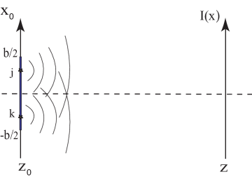
Figure 12: A large number of independent point sub-sources, such as the $j$th and $k$th, are randomly distributed on the plane of a thermal source. These point sub-sources randomly radiate independent spherical waves to the object and image planes, respectively. Due to the chaotic nature of the source, these independent sub-intensities simply added together yielding a constant total intensity in space and in time on any transverse planes.

To simplify the picture we assume the source in 1-D with a large number of independent point sub-sources randomly distributed from $-b/2$ to $b/2$. Each point sub-source, such as the $j$th and the $k$th sub-source, randomly radiates independent spherical waves to the object and image planes, respectively. Due to the chaotic nature of the source, these independent and incoherent sub-intensities simply add together yielding a constant total intensity spatially and temporally on any transverse plane. The more chaotic sub-fields that contribute to the intensity sum, the less value of $\Delta I/I$ is expected. For any two transverse planes, such as the object and the image planes in Fig. 9, each with independent and randomly distributed intensities, statistically, there is no reason to expect any spatial or temporal correlations. What is the physical cause that forces a twice large probability for the thermal radiation to jointly appear at $\vec{\rho}_{1}=\vec{\rho}_{\textrm{obj}}$?

In fact, we have been facing this question since 1956, after the discovery of Hanbury Brown and Twiss (HBT). The lensless ghost imaging setup looks similar to that of the historical HBT spatial interferometer which was used for measuring the angular size of distant stars. A significant difference is that the lensless ghost imaging measurement is in near-field for imaging purposes [5]. The HBT experiment created quite a surprise in the physics community with an enduring debate about the classical or quantum nature of the phenomenon [11][12].

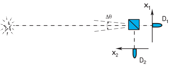
Figure 13: Schematic of the historical Hanbury Brown and Twiss experiment which measures the transverse spatial correlation of far-field thermal radiation.

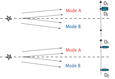
Figure 14: A phenomenological interpretation of the historical HBT experiment. Upper: the two photodetectors receive identical modes of the far-field radiation and thus experience identical intensity fluctuations. The joint measurement of $D_{1}$ and $D_{2}$ gives a maximum value of $\langle\Delta I_{1}\Delta I_{2}\rangle$. Lower: the two photodetectors receive different modes of the far-field radiation. In this case the joint measurement gives $\langle\Delta I_{1}\Delta I_{2}\rangle=0$. Unfortunately, this hand-waving interpretation does not reflect the correct physics in the case of $\Delta\theta\neq 0$. For a finite angular sized source, there is no chance, at least realistically, for $D_{1}$ and $D_{2}$ to receive radiation from a single radiation mode only. Nevertheless, the above theory has convinced us to believe that the observation of the intensity fluctuation correlation only takes place in the far-field zone of the thermal source.

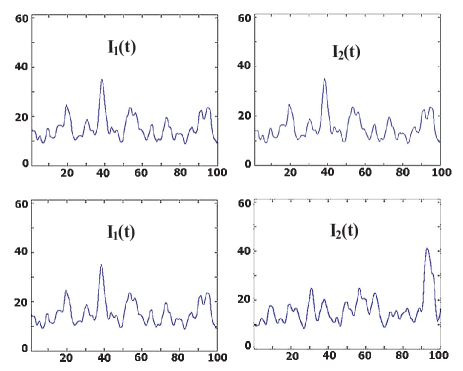
Figure 15: Schematic illustration of the light intensities $I_{1}(t)$ at $D_{1}$ and $I_{2}(t)$ at $D_{2}$. The two upper (lower) curves of $I(t)$ corresponds to the upper (lower) configuration in Fig 14.

Figure 13 is a schematic of the historical HBT experiment which measures the transverse spatial correlation of far-field thermal radiation. Performing the measurement in 1-D by scanning photodetectors $D_{1}$ and/or $D_{2}$ along the axes $x_{1}$ and $x_{2}$, the second-order transverse spatial correlation function $G^{(2)}(x_{1},x_{2})$ was found to be

$$G^{(2)}(x_{1},x_{2})\sim I_{0}^{2}\,\Big{\{}1+sinc^{2}\big{[}\,\frac{\pi\Delta\theta(x_{1}-x_{2})}{\lambda}\,\big{]}\Big{\}},$$ (33)

where $\Delta\theta$ is the angular size of the star, $\lambda$ the wavelength of the radiation. The far-field HBT correlation of Eq. (33) has been interpreted as the result of classical statistical correlation of the intensity fluctuations

$$\langle\,I_{1}I_{2}\,\rangle=\langle(\bar{I}_{1}+\Delta I_{1})(\bar{I}_{2}+\Delta I_{2})\rangle=\bar{I}_{1}\bar{I}_{2}+\langle\,\Delta I_{1}\Delta I_{2}\,\rangle,$$

where $\bar{I}_{1}$ and $\bar{I}_{2}$ are the mean intensities of the radiation measured by photodetectors $D_{1}$ and $D_{2}$, respectively. The second term in Eq. (33), $I_{0}^{2}\,sinc^{2}[\pi\Delta\theta(x_{1}-x_{2})/\lambda]$, is phenomenologically interpreted as the intensity fluctuation correlation $\langle\Delta I_{1}\Delta I_{2}\rangle$ in classical theory. For visible wavelengths and large values of $\Delta\theta$ this function quickly drops from its maximum to minimum when $x_{1}-x_{2}$ moves from zero to a value such that $\Delta\theta(x_{1}-x_{2})/\lambda=1$. In this situation we effectively have a “point-to-point” relationship between the $x_{1}$ and $x_{2}$ axes: for each point on the $x_{1}$ there exists only one point on the $x_{2}$ that may have a nonzero intensity fluctuation correlation.

The well-accepted interpretation of the HBT phenomenon is the following: in HBT the measurement is taken in the far-field zone of the radiation source, which is equivalent to the Fourier transform plane. When $D_{1}$ ($D_{2}$) is scanned in the neighborhood of $x_{1}=x_{2}$, the two detectors measure the same mode of the radiation field. The measured intensities have the same fluctuations and yield a maximum value of $\langle\Delta I_{1}\Delta I_{2}\rangle$. The two upper curves of $I(t)$ in Fig. 15 schematically illustrate this situation. When the two photodetectors move apart from $x_{1}=x_{2}$, $D_{1}$ and $D_{2}$ measure different modes of the radiation field. In this case, the measured two modes may have completely different fluctuations. The measurement yields $\langle\Delta I_{1}\Delta I_{2}\rangle=0$ and gives $\langle I_{1}I_{2}\rangle=\bar{I}_{1}\bar{I}_{2}$. This situation is illustrated in the two lower curves of $I(t)$ in Fig. 15. Unfortunately, this hand-waving interpretation does not reflect the correct physics in the case of $\Delta\theta\neq 0$. For a finite angular sized source, there is no chance, at least realistically, for $D_{1}$ and $D_{2}$ to receive radiation from a single radiation mode only. Nevertheless, the above theory has convinced us to believe that the observation of the intensity fluctuation correlation only takes place in the far-field zone of the thermal source.

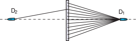
Figure 16: Modified near-field HBT measurement - an unfolded Klyshko picture of the setup. Assuming a large sized disk-like near-field chaotic source, each point on the disk can be considered as an independent sub-source. It is easy to see that (1) $D_{1}$ and $D_{2}$ are capable of receiving radiation from a large number of sub-sources; and (2) $D_{1}$ and $D_{2}$ have more chances to be triggered jointly by radiations from different sub-sources; (3) The ratio between the joint-detections triggered by radiation from a single sub-source and from different sub-sources is roughly $N/N^{2}=1/N$ in any transverse position of $D_{1}$ and $D_{2}$.

What will happen if we move the photodetectors $D_{1}$ and $D_{2}$ to the “near-field” as shown in the unfolded schematic of Fig. 16? Does this hand-waving argument still predict the point-to-point correlation in this situation? We consider a disk-like thermal source with a large number of independent and randomly radiating point sub-sources and assume the radiations coming from the same sub-source have the same intensity fluctuation, and the radiations coming from different sub-sources have different intensity fluctuations. It is easy to see that in the near-field, (1) each photodetector, $D_{1}$ and $D_{2}$, is capable of receiving radiations from a large number of sub-sources; and (2) $D_{1}$ and $D_{2}$, have more chances to be triggered jointly by radiation from different sub-sources; (3) The ratio between the joint-detections triggered by radiation from a single sub-source and from different sub-sources is roughly $N/N^{2}=1/N$ in any transverse position of $D_{1}$ and $D_{2}$. For a large value of $N$ the contribution of joint-detections triggered by radiation from a single sub-source in any transverse position of $D_{1}$ and $D_{2}$ has the same negligible value $\langle\Delta I_{1}\Delta I_{2}\rangle/\bar{I}_{1}\bar{I}_{2}\sim 0$. Following the above philosophy, the near-field $G^{(2)}(\vec{\rho}_{1},\vec{\rho}_{2})$ should be a constant for any chosen transverse coordinates $\vec{\rho}_{1}$ and $\vec{\rho}_{2}$. The experimental observations, however, have shown a different story.

The nontrivial near-field point-to-point correlation was experimentally observed in a modified HBT experiment by Scarcelli et al. in 2005 before the near-field lensless ghost imaging demonstration. The modified HBT has a similar experimental setup as that of the historical HBT of Fig. 13, except replacing the distant star with a near-field disk-like chaotic source. This light source has a considerably large angular diameter from the view of the photodetectors $D_{1}$ and $D_{2}$. The point photodetectors $D_{1}$ and $D_{2}$ are scannable along the axes of $x_{1}$ and $x_{2}$, respectively. The frequency bandwidth $\Delta\omega$ of this thermal source is chosen to be narrow enough to achieve $\sim$$\mu$s correlation width of $G^{(2)}(t_{1}-t_{2})$ which is shown in Fig. 17.

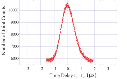
Figure 17: $G^{(2)}(t_{1}-t_{2})$ of a chaotic source. The temporal correlation width is measured $\sim 0.5\mu$s, which means that unless $t_{1}-t_{2}>0.5\mu$s, the value of $G^{(2)}(t_{1}-t_{2})$ will stay at the neighborhood of its maximum.

This means to change $G^{(2)}$ from its maximum (minimum) value to minimum (maximum) value requires a few hundred meters optical delay in the arm of either $D_{1}$ or $D_{2}$. The transverse intensity distributions were examined before the measurement of transverse correlation. The counting rate (weak light condition) or the output photocurrent (bright light condition) of each individual photodetector was found to be constant, i.e., $I(\vec{\rho}_{1})\sim$ constant and $I(\vec{\rho}_{2})\sim$ constant by scanning $D_{1}$ and $D_{2}$ in the transverse planes of $z_{1}=z_{0}$ and $z_{2}=z_{0}$, respectively. There is no surprise to have constant $I(\vec{\rho}_{1})$ and $I(\vec{\rho}_{2})$. The physics has been clearly illustrated in Fig. 12. By using this kind of chaotic source, Scarcelli et al. measured the 1-D near-field normalized transverse spatial correlation of $g^{(2)}(x_{1}-x_{2})$ by scanning $D_{1}$ in the neighborhood of $x_{1}=x_{2}$. The measurements confirmed the point-to-“spot” correlation of

$$g^{(2)}(x_{1}-x_{2})\sim 1+sinc^{2}\big{[}\,\frac{\pi\Delta\theta(x_{1}-x_{2})}{\lambda}\,\big{]},$$ (34)

where, again, $\Delta\theta$ is the angular diameter of the near-field disk-like chaotic source. It is worth emphasizing that $g^{(2)}(x_{1}-x_{2})$ dependents on $x_{1}-x_{2}$ only. Taking $x_{1}-x_{2}=$ constant, $g^{(2)}(x_{1}-x_{2})$ is invariant under the displacements of transverse coordinates.

A simplified summary of the experimental observation is shown in Fig. 18: (1) In the upper figure, $D_{1}$ and $D_{2}$ are placed at equal distances from the source and aligned symmetrically on the optical axis. The normalized joint-detection, or the value of $g^{(2)}$ achieved its maximum of $\sim 2$. (2) In the middle figure, $D_{1}$ is moved up a few millimeters to a non-symmetrical position, the normalized joint-detection, or the value of $g^{(2)}$ is measured to be $\sim 1$.

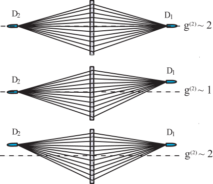
Figure 18: Schematic of the near-field spatial correlation measurement of Scarcelli et al. Upper: $g^{(2)}\sim 2$, where $D_{1}$ and $D_{2}$ are placed at equal distances from the source and aligned symmetrically on the optical axis. In the spirit of the traditional interpretation of HBT the intensities measured by $D_{1}$ and $D_{2}$ must have same fluctuations as shown in the figure. Middle: $g^{(2)}\sim 1$, where $D_{1}$ is moved up a few millimeters to an asymmetrical position. In the spirit of the traditional interpretation of HBT the intensities measured by $D_{1}$ and $D_{2}$ must have different fluctuations. Lower: $g^{(2)}\sim 2$, where $D_{2}$ is moved up to a symmetrical position with respect to $D_{1}$, again. In the spirit of the traditional interpretation of HBT the intensities measured by $D_{1}$ and $D_{2}$ must have same fluctuations again. What is the physical cause of the changes of the intensity fluctuations then? Remember the $G^{(2)}(t_{1}-t_{2})$ function has a width of $\sim 0.5\mu$, see Fig. 17.

(3) In the lower figure, $D_{2}$ is moved a few millimeters up to a symmetrical position with respect to $D_{1}$. The normalized joint-detection, or the value of $g^{(2)}$ turned back to its maximum of $\sim 2$ again.

It is easy to see that the classical theory of statistical correlation of intensity fluctuations is facing difficulties in explaining the experimental results. In near-field $D_{1}$ and $D_{2}$ receive the same large number of modes at any $\vec{\rho}_{1}$ and $\vec{\rho}_{2}$. In the spirit of the traditional interpretation of HBT, there seems no reason to have a different intensity fluctuation correlation between $\vec{\rho}_{1}=\vec{\rho}_{2}$ and $\vec{\rho}_{1}\neq\vec{\rho}_{2}$ for the $G^{(2)}$ function shown in Fig. 17. In the upper measurement, we have obtained the maximum value of $g^{(2)}\sim 2$ at $z_{1}=z_{2}$ and $x_{1}=x_{2}$, which indicates the achievement of a maximum intensity fluctuation correlation as shown in Fig. 17 with $|t_{1}-t_{2}|\sim 0$. In the middle measurement, $g^{(2)}\sim 1$ indicates a minimum intensity fluctuation correlation by moving $D_{1}$ a few millimeters up, which means the intensities measured by $D_{1}$ and $D_{2}$ must have different fluctuations. In the lower measurement $D_{2}$ is moved up a few millimeters to a new symmetrical position with respect to $D_{1}$, the measurements obtain $g^{(2)}\sim 2$ again. The intensities measured by $D_{1}$ and $D_{2}$ must have same fluctuations again. What is the physical cause of the changes of the intensity fluctuations then? Remember the $G^{(2)}(t_{1}-t_{2})$ function has a width of $\sim 0.5\mu$.

For half a century since 1956, it has been believed that the HBT correlation is observable in the far-field only. It was quite a surprise that in 2005 Scarcelli et al. successfully demonstrated a near-field point-to-point transverse correlation of chaotic light, indicating that the nontrivial HBT spatial correlation is observable in the near-field and is useful for reproducing ghost images in a nonlocal manner. The experiment of Scarcelli et al. raised a question: “Can two-photon correlation of chaotic light be considered as correlation of intensity fluctuations?” [5] At least, this experiment suggested we reexamine the relationship between the quantum mechanical concept of joint-detection probability with the classical concept of intensity fluctuation correlation. It seems that jointly observing a pair of photons at space-time point $(\mathbf{r}_{1},t_{1})$ and $(\mathbf{r}_{2},t_{2})$ is perhaps only phenomenologically connected but not physically caused by the classical statistical correlation of intensity fluctuations. The point-to-point image-forming correlation is more likely the result of an interference. In the view of two-photon interference, far-field is not a necessary condition for observing the partial point-to-point correlation of thermal light. Furthermore, it is quite common in two-photon interference type experiments to observe constant counting rates or intensities in individual photodetectors $D_{1}$ and $D_{2}$, respectively, and simultaneously observe nontrivial space-time correlation in the joint-detection between $D_{1}$ and $D_{2}$. These observations are consistent with the quantum theory of two-photon interferometry [9].

4.2 Quantum theory of thermal light ghost imaging

According to the quantum theory of light, the observed partial point-to-point image-forming correlation is the result of multi-photon interference. In Glauber’s theory of photo-detection [20], an idealized point photodetector measures the probability of observing a photo-detection event at space-time point $(\mathbf{r},t)$

$$G^{(1)}(\mathbf{r},t)=tr{\big{\{}\hat{\rho}\,E^{(-)}(\mathbf{r},t)E^{(+)}(\mathbf{r},t)\big{\}}},$$ (35)

where $\hat{\rho}$ is the density operator which characterizes the state of the quantized electromagnetic field, $E^{(-)}(\mathbf{r},t)$ and $E^{(+)}(\mathbf{r},t)$ the negative and positive field operators at space-time coordinate $(\mathbf{r},t)$. The counting rate of a point photon counting detector, or the output current of a point analog photodetector, is proportional to $G^{(1)}(\mathbf{r},t)$. A joint-detection of two independent point photodetectors measures the probability of observing a joint-detection event of two photons at space-time points $(\mathbf{r}_{1},t_{1})$ and $(\mathbf{r}_{2},t_{2})$

$$G^{(2)}(\mathbf{r}_{1},t_{1};\mathbf{r}_{2},t_{2})=tr{\big{\{}\hat{\rho}\,E^{(-)}(\mathbf{r}_{1},t_{1})E^{(-)}(\mathbf{r}_{2},t_{2})E^{(+)}(\mathbf{r}_{2},t_{2})E^{(+)}(\mathbf{r}_{1},t_{1})\big{\}}},$$ (36)

where $(\mathbf{r}_{j},t_{j})$, $j=1,2$, is the space-time coordinate of the $j$th photo-detection event. The coincidence counting rate of two photon counting detectors, or the output reading of a linear multiplier (RF mixer) between two photodetectors, is proportional to $G^{(2)}(\mathbf{r}_{1},t_{1};\mathbf{r}_{2},t_{2})$. To calculate the partial point-to-point correlation between the object plane and the image plane, we need (1) to estimate the state, or the density matrix, of the thermal radiation; and (2) to propagate the field operators from the radiation source to the object and the image planes. We will first calculate the state of thermal radiation at the single-photon level for photon counting measurements to explore the physics behind ghost imaging as two-photon interference and then generalize the result to any intensity of thermal radiation.

We assume a large transverse sized chaotic source consisting of a large number of independent and randomly radiating point sub-sources. Each point sub-source may also consist of a large number of independent atoms that are ready for two-level atomic transitions in a random manner. Most of the time, the atoms are in their ground state. There is, however, a small chance for each atom to be excited to a higher energy level $E_{2}$ ($\Delta E_{2}\neq 0$) and later return back to its ground state $E_{1}$. It is reasonable to assume that each atomic transition generates a field in the following single-photon state

$$|\,\Psi\,\rangle\simeq|\,0\,\rangle+\epsilon\,\sum_{\mathbf{k},s}\,f(\mathbf{k},s)\,\hat{a}^{{\dagger}}_{\mathbf{k},s}\,|\,0\,\rangle,$$ (37)

where $|\epsilon|\ll 1$ is the probability amplitude for the atomic transition, $f(\mathbf{k},s)=\langle\,\Psi_{\mathbf{k},s}\,|\,\Psi\,\rangle$ is the probability amplitude for the radiation field to be in the single-photon state of wave number ${\mathbf{k}}$ and polarization $s$: $|\,\Psi_{\mathbf{k},s}\,\rangle=|\,1_{\mathbf{k},s}\,\rangle=\hat{a}^{{\dagger}}_{\mathbf{k},s}\,|\,0\,\rangle$. For this simplified two-level system, the density matrix that characterizes the state of the radiation field excited by a large number of possible atomic transitions is thus

$$\hat{\rho} =\prod_{t_{0j}}\,\Big{\{}|\,0\,\rangle+\epsilon\sum_{\mathbf{k},s}\,f(\mathbf{k},s)\,e^{-i\omega t_{0j}}\,\hat{a}_{\mathbf{k},s}^{{\dagger}}\,|\,0\,\rangle\,\Big{\}}$$ (38)

$$\times\,\prod_{t_{0k}}\,\Big{\{}\langle\,0\,|\,+\epsilon^{\ast}\sum_{\mathbf{k}^{\prime},s^{\prime}}\,f(\mathbf{k}^{\prime},s^{\prime})\,e^{i\omega^{\prime}t_{0k}}\,\langle\,0\,|\hat{a}_{\mathbf{k}^{\prime},s^{\prime}}\,\Big{\}}$$

$$\simeq\Big{\{}|\,0\,\rangle+\epsilon[\sum_{t_{oj}}\sum_{\mathbf{k},s}\,f(\mathbf{k},s)\,e^{-i\omega t_{0j}}\,\hat{a}_{\mathbf{k},s}^{{\dagger}}\,|\,0\,\rangle]+\epsilon^{2}[...]\Big{\}}$$

$$\times\,\,\Big{\{}\langle\,0\,|\,+\epsilon^{\ast}[\sum_{t_{ok}}\sum_{\mathbf{k}^{\prime},s^{\prime}}\,f(\mathbf{k}^{\prime},s^{\prime})\,e^{i\omega^{\prime}t_{0k}}\,\langle\,0\,|\hat{a}_{\mathbf{k}^{\prime},s^{\prime}}]+\epsilon^{\ast 2}[...]\Big{\}},$$

where $e^{-i\omega t_{0j}}$ is a random phase factor associated with the jth atomic transition. Since $\left|\epsilon\right|\ll 1$, it is a good approximation to keep the necessary lower-order terms of $\epsilon$ in Eq. (38). After summing over $t_{0j}$ ($t_{0k}$) by taking into account all its possible values we obtain

$$\hat{\rho} \simeq|\,0\,\rangle\langle\,0\,|+\left|\epsilon\right|^{2}\sum_{\mathbf{k,s}}\left|f(\mathbf{k,s})\right|^{2}|\,1_{\mathbf{k,s}}\,\rangle\langle\,1_{\mathbf{k,s}}\,|$$

$$+\left|\epsilon\right|^{4}\sum_{\mathbf{k,s}}\sum_{\mathbf{k}^{\prime},s^{\prime}}\left|f(\mathbf{k,s})\right|^{2}\left|f(\mathbf{k}^{\prime},s^{\prime})\right|^{2}|\,1_{\mathbf{k,s}}1_{\mathbf{k}^{\prime},s^{\prime}}\,\rangle\langle\,1_{\mathbf{k},s}1_{\mathbf{k}^{\prime},s^{\prime}}\,|+...$$ (39)

Similar to our earlier discussion we will focus our calculation on the transverse correlation by assuming a narrow enough frequency bandwidth in Eq. (4.2). In the experiments of Scarcelli et al. the coherence time of the radiation was chosen $\sim$$\mu$s, the maximum achievable optical path differences $\sim$ps by the scanning of $D_{1}$ and $D_{2}$, and the response time of the photodetectors is much less than the coherence time. The transverse spatial correlation measurement is under the condition of achieving a maximum temporal coherence of $G^{(2)}(t_{1}-t_{2})\sim 2$ during the scanning of $D_{1}$ and $D_{2}$ at any $\vec{\rho}_{1}$ and $\vec{\rho}_{2}$. In the photon counting regime, under the above condition, it is reasonable to model the thermal light in the following mixed state

$$\hat{\rho}\simeq|\,0\,\rangle\langle\,0\,|+\left|\epsilon\right|^{2}\sum_{\vec{\kappa}}\hat{a}^{\dagger}(\vec{\kappa})|\,0\,\rangle\langle\,0\,|\hat{a}(\vec{\kappa})+\left|\epsilon\right|^{4}\sum_{\vec{\kappa}}\sum_{\vec{\kappa}^{\prime}}\hat{a}^{\dagger}(\vec{\kappa})\hat{a}^{\dagger}(\vec{\kappa}^{\prime})\,|\,0\,\rangle\langle\,0\,|\,\hat{a}(\vec{\kappa}^{\prime})\hat{a}(\vec{\kappa}).$$ (40)

Basically we are modeling the light source as an incoherent statistical mixture of single-photon states and two-photon states with equal probability of having any transverse momentum. The spatial part of the second-order coherence function is thus calculated as

$$G^{(2)}(\vec{\rho}_{1},z_{1};\vec{\rho}_{2},z_{2}) =tr{[\,\hat{\rho}\,E^{(-)}(\vec{\rho}_{1},z_{1})E^{(-)}(\vec{\rho}_{2},z_{2})E^{(+)}(\vec{\rho}_{2},z_{2})E^{(+)}(\vec{\rho}_{1},z_{1})\,]}$$

$$=\sum_{\vec{\kappa},\vec{\kappa}^{\prime}}\langle 1_{\vec{\kappa}}1_{\vec{\kappa}^{\prime}}|E^{(-)}(\vec{\rho}_{1},z_{1})E^{(-)}(\vec{\rho}_{2},z_{2})E^{(+)}(\vec{\rho}_{2},z_{2})E^{(+)}(\vec{\rho}_{1},z_{1})|1_{\vec{\kappa}}1_{\vec{\kappa}^{\prime}}\rangle$$

$$\equiv\sum_{\vec{\kappa},\vec{\kappa}^{\prime}}\big{|}\Psi_{\vec{\kappa},\vec{\kappa}^{\prime}}(\vec{\rho}_{1},z_{1};\vec{\rho}_{2},z_{2})\big{|}^{2},$$ (41)

where we have defined an effective two-photon wavefunction in transverse spatial coordinates

$$\Psi_{\vec{\kappa},\vec{\kappa}^{\prime}}(\vec{\rho}_{1},z_{1};\vec{\rho}_{2},z_{2})=\langle 0|E^{(+)}(\vec{\rho}_{2},z_{2})E^{(+)}(\vec{\rho}_{1},z_{1})|1_{\vec{\kappa}}1_{\vec{\kappa}^{\prime}}\rangle.$$ (42)

The transverse part of the electric field operator can be written as

$$E^{(+)}(\vec{\rho}_{j},z_{j})\propto\sum_{\vec{\kappa}}\,g_{j}(\vec{\rho}_{j},z_{j};\vec{\kappa})\,\hat{a}(\vec{\kappa}),$$ (43)

again, $g_{j}(\vec{\rho}_{j},z_{j};\vec{\kappa})$ is the Green’s function. Substituting the field operators into Eq. (42) we have

$$\Psi_{\vec{\kappa},\vec{\kappa}^{\prime}}(\vec{\rho}_{1},z_{1};\vec{\rho}_{2},z_{2})=\frac{1}{\sqrt{2}}\big{[}g_{2}(\vec{\rho}_{2},z_{2};\vec{\kappa})g_{1}(\vec{\rho}_{1},z_{1};\vec{\kappa}^{\prime})+g_{2}(\vec{\rho}_{2},z_{2};\vec{\kappa}^{\prime})g_{1}(\vec{\rho}_{1},z_{1};\vec{\kappa})\big{]}$$ (44)

and

$$G^{(2)}(\vec{\rho}_{1},z_{1};\vec{\rho}_{2},z_{2})=\sum_{\vec{\kappa},\vec{\kappa}^{\prime}}\Big{|}\frac{1}{\sqrt{2}}\big{[}g_{2}(\vec{\rho}_{2},z_{2};\vec{\kappa})g_{1}(\vec{\rho}_{1},z_{1};\vec{\kappa}^{\prime})+g_{2}(\vec{\rho}_{2},z_{2};\vec{\kappa}^{\prime})g_{1}(\vec{\rho}_{1},z_{1};\vec{\kappa})\big{]}\Big{|}^{2},$$ (45)

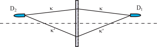
Figure 19: Schematic illustration of two-photon interference: a superposition between two-photon amplitudes $g_{2}(\vec{\rho}_{2},z_{2}\vec{\kappa})g_{1}(\vec{\rho}_{1},z_{1};\vec{\kappa}^{\prime})$ and $g_{2}(\vec{\rho}_{2},z_{2};\vec{\kappa}^{\prime})g_{1}(\vec{\rho}_{1},z_{1};\vec{\kappa})$. It is clear that the amplitudes $g_{2}(\vec{\rho}_{2},z_{2};\vec{\kappa})g_{1}(\vec{\rho}_{1},z_{1};\vec{\kappa}^{\prime})$ and $g_{2}(\vec{\rho}_{2},z_{2};\vec{\kappa}^{\prime})g_{1}(\vec{\rho}_{1},z_{1};\vec{\kappa})$ will experience equal optical path propagation and superpose constructively when $D_{1}$ and $D_{2}$ are located at $\vec{\rho}_{1}\simeq\vec{\rho}_{2}$ and $z_{1}\simeq z_{2}$. This nonlocal superposition has no classical correspondence.

representing the key result for our understanding of the phenomenon. Eqs. (44) and (45) indicates an interference between two alternatives, different yet indistinguishable, which leads to a joint photo-detection event. This interference phenomenon is not, as in classical optics, due to the superposition of electromagnetic fields at a local point of space-time. This interference is the result of the superposition between $g_{2}(\vec{\rho}_{2},z_{2};\vec{\kappa})g_{1}(\vec{\rho}_{1},z_{1};\vec{\kappa}^{\prime})$ and $g_{2}(\vec{\rho}_{2},z_{2};\vec{\kappa}^{\prime})g_{1}(\vec{\rho}_{1},z_{1};\vec{\kappa})$, the so-called two-photon amplitudes, non-classical entities that involve both arms of the optical setup as well as two distant photo-detection events at ($\vec{\rho}_{1},z_{1}$) and ($\vec{\rho}_{2},z_{2}$), respectively. Examining the effective wavefunction of Eq. (44), we find this symmitrized effective wavefunction plays the same role as that of the symmitrized wavefunction of identical particles in quantum mechanics. This peculiar nonlocal superposition has no classical correspondence, and makes the type-two ghost image turbulence-free, i.e., any phase disturbance in the optical path has no influence on the ghost image [24]. Fig. 19 schematically illustrates the two alternatives for a pair of mode $\vec{\kappa}$ and $\vec{\kappa}^{\prime}$ to produce a joint photo-detection event: $\vec{\kappa}1\times\vec{\kappa}^{\prime}2$ and $\vec{\kappa}2\times\vec{\kappa}^{\prime}1$. The superposition of each pair of these amplitudes produces an individual sub-interference-pattern in the joint-detection space of $(\vec{\rho}_{1},z_{1},t_{1};\vec{\rho}_{2},z_{2},t_{2})$. A large number of these sub-interference-patterns simply add together resulting in a nontrivial $G^{(2)}(\vec{\rho}_{1},z_{1};\vec{\rho}_{2},z_{2})$ function. It is easy to see that each pair of the two-photon amplitudes, illustrated in Fig. 19, will superpose constructively whenever $D_{1}$ and $D_{2}$ are placed in the positions satisfying $\vec{\rho}_{1}\simeq\vec{\rho}_{2}$ and $z_{1}\simeq z_{2}$; and consequently, $G^{(2)}(\vec{\rho}_{1},z_{1};\vec{\rho}_{2},z_{2})$ achieves its maximum value as the result of the sum of these individual constructive interferences. In other coordinates, however, the superposition of each individual pair of the two-photon amplitudes may yield different values between constructive maximum and destructive minimum due to unequal optical path propagation, resulting in an averaged sum.

Before calculating $G^{(2)}(\vec{\rho}_{1},z_{1};\vec{\rho}_{2},z_{2})$ we examine the single counting rate of the point photodetectors $D_{1}$ and $D_{2}$ which are placed at ($\vec{\rho}_{1},z_{1})$ and ($\vec{\rho}_{2},z_{2}$), respectively. With reference to the experimental setup of Fig. 9, the Green’s function of free-propagation is derived in the Appendix

$$g_{1}(\vec{\rho}_{1},z_{1};\vec{\kappa})=\int d\vec{\rho}_{s}\,\Big{\{}\frac{-i\omega}{2\pi c}\,\frac{e^{i\frac{\omega}{c}z_{1}}}{z_{1}}\,e^{i\frac{\omega}{2cz_{1}}|\vec{\rho}_{1}-\vec{\rho}_{s}|^{2}}\Big{\}}\,e^{-i\vec{\kappa}\cdot\vec{\rho}_{s}},$$

$$g_{2}(\vec{\rho}_{2},z_{2};\vec{\kappa})=\int d\vec{\rho^{\prime}_{s}}\,\Big{\{}\frac{-i\omega}{2\pi c}\,\frac{e^{i\frac{\omega}{c}z_{2}}}{z_{2}}\,e^{i\frac{\omega}{2cz_{2}}|\vec{\rho}_{2}-\vec{\rho^{\prime}_{s}}|^{2}}\Big{\}}\,e^{-i\vec{\kappa}\cdot\vec{\rho^{\prime}_{s}}},$$

where $\vec{\rho}_{s}$ is the transverse vector in the source plane, and the field has propagated from the source to the $\vec{\rho}_{1}$ plane and $\vec{\rho}_{2}$ plane in arms 1 and 2, respectively. The single detector counting rate or the output photocurrent is proportional to $G^{(1)}(\mathbf{r},t)$ as shown in Eq. (35),

$$G^{(1)}(\vec{\rho}_{j},z_{j}) =tr{\big{\{}\hat{\rho}\,E^{(-)}(\vec{\rho}_{j},z_{j})E^{(+)}(\vec{\rho}_{j},z_{j})\big{\}}}$$

$$\propto\sum_{\vec{\kappa}}\langle\,0\,|\,\hat{a}(\vec{\kappa})\,E^{(-)}(\vec{\rho}_{j},z_{j})E^{(+)}(\vec{\rho}_{j},z_{j})\,\hat{a}^{\dagger}(\vec{\kappa})|\,0\,\rangle$$

$$\sim\text{constant},$$ (46)

where $j=1,2$ indicating the $j$th photodetector.

Although $G^{(1)}(\vec{\rho}_{1},z_{1})$ and $G^{(1)}(\vec{\rho}_{2},z_{2})$ are both constants, $G^{(2)}(\vec{\rho}_{1},z_{1};\vec{\rho}_{2},z_{2})$ turns to be a nontrivial function of $(\vec{\rho}_{1},z_{1})$ and ($\vec{\rho}_{2},z_{2}$),

$$G^{(2)}(\vec{\rho}_{1},z_{1};\vec{\rho}_{2},z_{2}) =\sum_{\vec{\kappa},\vec{\kappa}^{\prime}}\Big{|}\frac{1}{\sqrt{2}}\big{[}g_{2}(\vec{\rho}_{2},z_{2};\vec{\kappa})g_{1}(\vec{\rho}_{1},z_{1};\vec{\kappa}^{\prime})+g_{2}(\vec{\rho}_{2},z_{2};\vec{\kappa}^{\prime})g_{1}(\vec{\rho}_{1},z_{1};\vec{\kappa})\big{]}\Big{|}^{2}$$

$$\equiv G^{(1)}(\vec{\rho}_{1},z_{1})G^{(1)}(\vec{\rho}_{2},z_{2})+\big{|}G^{(1)}(\vec{\rho}_{1},z_{1};\vec{\rho}_{2},z_{2})\big{|}^{2},$$ (47)

where

$$\big{|}G^{(1)}(\vec{\rho}_{1},z_{1};\vec{\rho}_{2},z_{2})\big{|}^{2} =\big{|}\int d\vec{\kappa}\,\,g^{*}_{1}(\vec{\rho}_{1},z_{1};\vec{\kappa})\,g_{2}(\vec{\rho}_{2},z_{2};\vec{\kappa})\big{|}^{2}$$

$$\propto\big{|}\int d\vec{\rho}_{s}\,e^{-i\frac{\omega}{c}z_{1}}\,e^{-i\frac{\omega}{2cz_{1}}|\vec{\rho}_{1}-\vec{\rho}_{s}|^{2}}\,e^{i\frac{\omega}{c}z_{2}}\,e^{i\frac{\omega}{2cz_{2}}|\vec{\rho}_{2}-\vec{\rho}_{s}|^{2}}\big{|}^{2}.$$

If we choose the distances from the source to the two detectors to be equal ($z_{1}=z_{2}=d$), the above integral of $d\vec{\rho}_{s}$ yields a point-to-point correlation between the transverse planes $z_{1}=d$ and $z_{2}=d$,

$$\big{|}\,G^{(1)}_{12}(\vec{\rho}_{1};\vec{\rho}_{2})\,\big{|}^{2} \propto\Big{|}\int d\vec{\rho}_{s}\,e^{i\frac{\omega}{cd}(\vec{\rho}_{1}-\vec{\rho}_{2})\cdot\vec{\rho}_{s}}\,\Big{|}^{2}=somb^{2}\big{[}\frac{R}{d}\frac{\omega}{c}|\vec{\rho}_{1}-\vec{\rho}_{2}|\big{]}\sim\delta(\vec{\rho}_{1}-\vec{\rho}_{2}),$$ (48)

where the $\delta$-function is an approximation by assuming a large enough thermal source of angular size $\Delta\theta\sim R/d$ and high enough frequency $\omega$, such as a visible light source. The nontrivial $G^{(2)}$ function is therefore,

$$G^{(2)}(\vec{\rho}_{1};\vec{\rho}_{2})\sim 1+\delta(\vec{\rho}_{1}-\vec{\rho}_{2}).$$ (49)

In the ghost imaging experiment, the joint-detection counting rate is thus

$$R_{12}\propto\int d\vec{\rho}_{2}\,|A(\vec{\rho}_{2})|^{2}\,G^{(2)}(\vec{\rho}_{1};\vec{\rho}_{2})\sim R_{0}+|A(\vec{\rho}_{1})|^{2},$$ (50)

where $R_{0}$ is a constant and $A(\vec{\rho}_{2})$ is the aperture function of the object.

So far, we have successfully derived an analytical solution for ghost imaging with thermal radiation at the single-photon level. We have shown that the partial point-to-point correlation of thermal radiation is the result of a constructive-destructive interference caused by the superposition of two two-photon amplitudes, corresponding to two alternative ways for a pair of jointly measured photons to produce a joint-detection event. In fact the above analysis is not restricted to single-photon states. The partial point-to-point correlation of $G^{(2)}(\vec{\rho}_{1};\vec{\rho}_{2})$ is generally true for any order of quantized thermal radiation [25]. Now we generalize the calculation to an arbitrary quantized thermal field with occupation number from $n_{\mathbf{k,s}}=0$ to $n_{\mathbf{k,s}}\gg 1$ by keeping all higher order terms in Eq. (38). After summing over $t_{0j}$ and $t_{0k}$ the density matrix can be written as

$$\hat{\rho}=\sum_{\{n\}}\,p_{\{n\}}\,|\{n\}\rangle\langle\{n\}|,$$ (51)

where $p_{\{n\}}$ is the probability for the thermal field in the state

$$|\{n\}\rangle\equiv\prod_{\mathbf{k},s}|n_{\mathbf{k},s}\rangle=|n_{\mathbf{k},s}\rangle|n_{\mathbf{k}^{\prime},s^{\prime}}\rangle...|n_{\mathbf{k}^{\prime\prime...\prime},s^{\prime\prime...\prime}}\rangle.$$

The summation of Eq. (51) includes all possible modes $\mathbf{k}$, polarizations $s$, occupation numbers $n_{\mathbf{k},s}$ for the mode $(\mathbf{k},s)$ and all possible combinations of occupation numbers for different modes in a set of $\{n\}$. Substituting the field operators and the density operator of Eq. (51) into Eq. (35) we obtain the constant $G^{(1)}(\vec{\rho}_{j},z_{j},t_{j})$, $j=1,2$, which corresponds to the intensities $I(\vec{\rho}_{1},z_{1},t_{1})$ and $I(\vec{\rho}_{2},z_{2},t_{2})$,

$$\ \ \ \ G^{(1)}(\vec{\rho}_{j},z_{j},t_{j})$$

$$=\sum_{\{n\}}\int d\vec{\kappa}\int d\vec{\kappa}^{\prime}g_{j}^{*}(\vec{\rho}_{j},z_{1},t_{j};\vec{\kappa})g_{j}(\vec{\rho}_{j},z_{1},t_{j};\vec{\kappa}^{\prime})\,p_{\{n\}}\,\langle\{n\}|\,a(\vec{\kappa})a^{\dagger}(\vec{\kappa}^{\prime})\,|\{n\}\rangle$$

$$\propto\sum_{\{n\}}n_{\vec{\kappa}}\,n_{\vec{\kappa}^{\prime}}\int d\vec{\kappa}\ \big{|}\,g_{j}^{*}(\vec{\rho}_{j},z_{j},t_{j};\vec{\kappa})\,\big{|}^{2}$$

$$\simeq\text{constant}.$$ (52)

Although $G^{(1)}(\vec{\rho}_{1},z_{1},t_{1})$ and $G^{(1)}(\vec{\rho}_{2},z_{2},t_{2})$ are both constants, substituting the field operators and the density operator of Eq. (51) into Eq. (36), we obtain a nontrivial point-to-point correlation function of $G^{(2)}(\vec{\rho_{1}};\vec{\rho_{2}})$ at the two transverse planes $z_{1}=d$ and $z_{2}=d$,

$$\ \ \ \ G^{(2)}(\vec{\rho_{1}};\vec{\rho_{2}})$$

$$=\sum_{\{n\}}\int d\vec{\kappa}\int d\vec{\kappa}^{\prime}\int d\vec{\kappa}^{\prime\prime}\int d\vec{\kappa}^{\prime\prime\prime}g_{1}^{*}(\vec{\rho}_{1},z_{1};\vec{\kappa})g_{2}^{*}(\vec{\rho}_{2},z_{2};\vec{\kappa}^{\prime})g_{2}(\vec{\rho}_{2},z_{2};\vec{\kappa}^{\prime\prime})g_{1}(\vec{\rho}_{1},z_{1};\vec{\kappa}^{\prime\prime\prime})$$

$$\ \ \ \ \times\,p_{\{n\}}\,\langle\{n\}|\,a(\vec{\kappa})a(\vec{\kappa}^{\prime})a^{\dagger}(\vec{\kappa}^{\prime\prime})a^{\dagger}(\vec{\kappa}^{\prime\prime\prime})\,|\{n\}\rangle$$

$$\propto\sum_{\{n\}}n_{\vec{\kappa}}\,n_{\vec{\kappa}^{\prime}}\int d\vec{\kappa}\int d\vec{\kappa}^{\prime}\int d\vec{\kappa}^{\prime\prime}\int d\vec{\kappa}^{\prime\prime\prime}g_{1}^{*}(\vec{\rho}_{1},z_{1};\vec{\kappa})g_{2}^{*}(\vec{\rho}_{2},z_{2};\vec{\kappa}^{\prime})g_{2}(\vec{\rho}_{2},z_{2};\vec{\kappa}^{\prime\prime})g_{1}(\vec{\rho}_{1},z_{1};\vec{\kappa}^{\prime\prime\prime})$$

$$\ \ \ \ \times\,p_{\{n\}}(\delta_{\vec{\kappa}\vec{\kappa}^{\prime\prime\prime}}\delta_{\vec{\kappa}^{\prime}\vec{\kappa}^{\prime\prime}}+\delta_{\vec{\kappa}\vec{\kappa}^{\prime\prime}}\delta_{\vec{\kappa}^{\prime}\vec{\kappa}^{\prime\prime\prime}})$$

$$=\sum_{n_{\vec{\kappa}}n_{\vec{\kappa}^{\prime}}}p_{\{...n_{\vec{\kappa}}...n_{\vec{\kappa}^{\prime}}...\}}\,n_{\vec{\kappa}}\,n_{\vec{\kappa}^{\prime}}$$

$$\ \ \ \ \times\Big{\{}\int d\vec{\kappa}\int d\vec{\kappa}^{\prime}\,\Big{|}\frac{1}{\sqrt{2}}\,\big{[}g_{1}(\vec{\rho}_{1},z_{1};\vec{\kappa})g_{2}(\vec{\rho}_{2},z_{2};\vec{\kappa}^{\prime})+g_{2}(\vec{\rho}_{2},z_{2};\vec{\kappa})g_{1}(\vec{\rho}_{1},z_{1};\vec{\kappa}^{\prime})\big{]}\Big{|}^{2}\Big{\}}$$

$$\propto\Big{\{}1+somb^{2}\big{[}\frac{R}{d}\frac{\omega}{c}(\vec{\rho}_{1}-\vec{\rho}_{2})\big{]}\Big{\}}.$$ (53)

It is clear that in Eq. (4.2), the partial point-to-point correlation of thermal light is the result of a constructive-destructive interference between two quantum-mechanical amplitudes. We also note from Eq. (4.2) that the partial point-to-point correlation is independent of the occupation numbers, $\{n\}$, and the probability distribution, $p_{\{n\}}$, of the quantized thermal radiation.

It is interesting but not surprising to see that the effective two-photon wavefunction in bright light condition

$$\Psi_{\vec{\kappa},\vec{\kappa}^{\prime}}(\vec{\rho}_{1},z_{1};\vec{\rho}_{2},z_{2})=\frac{1}{\sqrt{2}}\big{[}g_{2}(\vec{\rho}_{2},z_{2};\vec{\kappa})g_{1}(\vec{\rho}_{1},z_{1};\vec{\kappa}^{\prime})+g_{2}(\vec{\rho}_{2},z_{2};\vec{\kappa}^{\prime})g_{1}(\vec{\rho}_{1},z_{1};\vec{\kappa})\big{]}$$

is the same as that of weak light at single-photon level. In fact, the above effective wavefunction does play the same role in specifying two different yet indistinguishable alternatives for the two annihilated photons contributing to a joint-detection event of $D_{1}$ and $D_{2}$, which implies that the partial point-to-point correlation is the result of two-photon interference in bright light condition. This nonlocal partial correlation indicates that a $50\%$ contrast ghost image is observable at bright light condition provided registering no more than one coincidence event within the joint-detection time window. This requirement can be easily achieved by using adjustable ND-filters with $D_{1}$ and $D_{2}$.

Quantum theory predicts and calculates the probability of observing a certain physical event. The output photocurrent of an idealized point photodetector is proportional to the probability of observing a photo-detection event at space-time point ($\mathbf{r},t$). The joint-detection between two idealized point photodetectors is proportional to the probability of observing a joint photo-detection event at space-time points ($\mathbf{r}_{1},t_{1}$) and ($\mathbf{r}_{2},t_{2}$). In most of the experimental situations, there exists more than one possible alternative ways to produce a photo-detection event, or a joint photo-detection event. These probability amplitudes, which are defined as the single-photon amplitudes and the two-photon amplitudes, respectively, are superposed to contribute to the final measured probability, and consequently determine the probability of observing a photo-detection event or a joint photo-detection event. In the view of quantum theory, whenever the state of the quantum system and the alternative ways to produce a photo-detection event or a joint photo-detection event are determined, the result of a measurement is determined. We may consider this as a basic criterion of quantum measurement theory.

4.3 A semiclassical model of nonlocal interference

The multi–photon interference nature of type-two ghost imaging can be seen intuitively from the superposition of paired-sub-fields of chaotic radiation. Let us consider a similar experimental setup as that of the modified HBT experiment of Scarcelli et al.. We assume a large angular sized disk-like chaotic source that contains a large number of randomly radiating independent point “sub-sources”, such as trillions of independent atomic transitions randomly distributed spatially and temporally. It should be emphasized that a large number of independent or incoherent sub-sources is the only requirement for type-two ghost imaging. What we need is an ensemble of point-sub-sources with random relative phases so that the sub-fields coming from these sub-sources are able to take all possible values of relative phases in their superposition. It is unnecessary to require the radiation source to have either nature or artificial intensity fluctuations at all. In this model, each point sub-source contributes to the measurement an independent spherical wave as a sub-field of complex amplitude $E_{j}=a_{j}e^{i\varphi_{j}}$, where $a_{j}$ is the real and positive amplitude of the $j$th sub-field and $\varphi_{j}$ is a random phase associated with the $j$th sub-field. We have the following picture for the source: (1) a large number of independent point-sources distribute randomly on the transverse plane of the source (counted spatially); (2) each point-source contains a large number of independently and randomly radiating atoms (counted temporally); (3) a large number of sub-sources, either counted spatially or temporally, may contribute to each of the independent radiation mode ($\vec{\kappa},\omega$) at $D_{1}$ and $D_{2}$ (counted by mode). The instantaneous intensity at space-time $(\mathbf{r}_{j},t_{j})$, measured by the $j$th idealized point photodetector $D_{j}$, $j=1,2$, is calculated as

$$I(\mathbf{r}_{j},t_{j}) =E^{*}(\mathbf{r}_{j},t_{j})E(\mathbf{r}_{j},t_{j})=\sum_{l}E^{*}_{l}(\mathbf{r}_{j},t_{j})\sum_{m}E_{m}(\mathbf{r}_{j},t_{j})$$

$$=\sum_{l=m}E^{*}_{l}(\mathbf{r}_{j},t_{j})E_{l}(\mathbf{r}_{j},t_{j})+\sum_{l\neq m}E^{*}_{l}(\mathbf{r}_{j},t_{j})E_{m}(\mathbf{r}_{j},t_{j}),$$ (54)

where the sub-fields are identified by the index $l$ and $m$ originated from the $l$ and $m$ sub-sources. The first term is a constant representing the sum of the sub-intensities, where the $l$th sub-intensity is originated from the $l$th sub-source. The second term adds the “cross” terms corresponding to different sub-sources. When taking into account all possible realizations of the fields, it is easy to find that the only surviving terms in the sum are these terms in which the field and its conjugate come from the same sub-source, i.e., the first term in Eq. (4.3). The second term in Eq. (4.3) vanishes if $\varphi_{l}-\varphi_{m}$ takes all possible values. We may write Eq. (4.3) into the following form

$$I(\mathbf{r}_{j},t_{j})=\langle I(\mathbf{r},t)\rangle+\Delta I(\mathbf{r},t),$$ (55)

where

$$\langle I(\mathbf{r},t)\rangle\equiv\langle\sum_{l}E^{*}_{l}(\mathbf{r}_{j},t_{j})\sum_{m}E_{m}(\mathbf{r}_{j},t_{j})\,\rangle=\sum_{l}E^{*}_{l}(\mathbf{r}_{j},t_{j})E_{l}(\mathbf{r}_{j},t_{j}).$$ (56)

The notation $\langle...\rangle$ denotes the mathematical expectation, when taking into account all possible realizations of the fields, i.e., taking into account all possible complex amplitudes for the large number of sub-fields in the superposition. In the probability theory, the expectation value of a measurement equals the mean value of an ensemble. In a real measurement, the superposition may not take all possible realizations of the fields and consequently the measured instantaneous intensity $I(\mathbf{r},t)$ may differ from its expectation value $\langle I(\mathbf{r},t)\rangle$ from time to time. The variation $\delta I(\mathbf{r},t)$ turns to be a random function of time. The measured $I(\mathbf{r},t)$ fluctuate randomly in the neighborhood of $\langle I(\mathbf{r},t)\rangle$ non-deterministically.

In the classical limit, a large number of independent and randomly radiated sub-sources contribute to the instantaneous intensity $I(\mathbf{r}_{j},t_{j})$. These large number of independent randomly distributed sub-fields may have taken all possible realizations of their complex amplitudes in the superposition. In this case the sum of the cross terms vanishes,

$$\Delta I(\mathbf{r},t)=\sum_{l\neq m}E^{*}_{l}(\mathbf{r}_{j},t_{j})E_{m}(\mathbf{r}_{j},t_{j})\simeq 0,$$ (57)

therefore,

$$I(\mathbf{r}_{j},t_{j})\simeq\sum_{l}E^{*}_{l}(\mathbf{r}_{j},t_{j})E_{l}(\mathbf{r}_{j},t_{j})=\langle I(\mathbf{r},t)\rangle.$$

Now we calculate the second-order correlation function $G^{(2)}(\mathbf{r}_{1},t_{1};\mathbf{r}_{2},t_{2})$, which is defined as

$$G^{(2)}(\mathbf{r}_{1},t_{1};\mathbf{r}_{2},t_{2}) \equiv\langle\sum_{j,k,l,m}E^{*}_{j}(\mathbf{r}_{1},t_{1})\,E_{k}(\mathbf{r}_{1},t_{1})E^{*}_{l}(\mathbf{r}_{2},t_{2})\,E_{m}(\mathbf{r}_{2},t_{2})\,\rangle,$$ (58)

where the notation $\langle\,...\,\rangle$, again, denotes an expectation operation by taking into account all possible realizations of the fields, i.e., averaging all possible complex amplitudes for the sub-fields in the superposition. In the following calculation we only take into account the random phases of the sub-fields without considering the amplitude variations. Due to the chaotic nature of the independent sub-sources, after taking into account all possible realizations of the phases associated with the sub-fields, the only surviving terms in the summation are those with: (1) $j=k,l=m$, (2) $j=m,k=l$. Therefore, $G^{(2)}(\mathbf{r}_{1},t_{1};\mathbf{r}_{2},t_{2})$ reduces to the sum of the following two groups:

$$G^{(2)}(\mathbf{r}_{1},t_{1};\mathbf{r}_{2},t_{2}) =\langle\,\sum_{j}\,E^{*}_{j}(\mathbf{r}_{1},t_{1})\,E_{j}(\mathbf{r}_{1},t_{1})\,\sum_{l}\,E^{*}_{l}(\mathbf{r}_{2},t_{2})\,E_{l}(\mathbf{r}_{2},t_{2})$$

$$\hskip 14.22636pt+\sum_{j}\,E^{*}_{j}(\mathbf{r}_{1},t_{1})\,E_{j}(\mathbf{r}_{2},t_{2})\,\sum_{l}\,E^{*}_{l}(\mathbf{r}_{2},t_{2})\,E_{l}(\mathbf{r}_{1},t_{1})\,\rangle$$

$$=\langle\,\sum_{j}\sum_{l}\,\Big{|}\frac{1}{\sqrt{2}}\big{[}E_{j}(\mathbf{r}_{1},t_{1})E_{l}(\mathbf{r}_{2},t_{2})+E_{l}(\mathbf{r}_{1},t_{1})E_{j}(\mathbf{r}_{2},t_{2})\big{]}\Big{|}^{2}\,\rangle.$$ (59)

It is not difficult to see the nonlocal nature of the superposition shown in Eq. (4.3). In Eq. (4.3), $G^{(2)}(\mathbf{r}_{1},t_{1};\mathbf{r}_{2},t_{2})$ is written as a superposition between the paired sub-fields $E_{j}(\mathbf{r}_{1},t_{1})E_{l}(\mathbf{r}_{2},t_{2})$ and $E_{l}(\mathbf{r}_{1},t_{1})E_{j}(\mathbf{r}_{2},t_{2})$. The first term in the superposition corresponds to the situation in which the field at $D_{1}$ was generated by the $jth$ sub-source, and the field at $D_{2}$ was generated by the $lth$ sub-source. The second term in the superposition corresponds to a different yet indistinguishable situation in which the field at $D_{1}$ was generated by the $lth$ sub-source, and the field at $D_{2}$ was generated by the $jth$ sub-source. Therefore, an interference is concealed in the joint measurement of $D_{1}$ and $D_{2}$, which physically occurs at two space-time points $(\mathbf{r}_{1},t_{1})$ and $(\mathbf{r}_{2},t_{2})$. The interference corresponds to $|E_{j1}E_{l2}+E_{l1}E_{j2}|^{2}$.

Figure 20: Schematic illustration of $\sum_{j,l}|E_{j1}E_{l2}+E_{l1}E_{j2}|^{2}$. It is clear that the amplitude pairs $j1\times l2$ with $l1\times j2$, where $j$ and $l$ represent all point sub-sources, pair by pair, will experience equal optical path propagation and superpose constructively when $D_{1}$ and $D_{2}$ are located at $\vec{\rho}_{1}\simeq\vec{\rho}_{2}$, $z_{1}\simeq z_{2}$. This interference is similar to symmetrizing the wavefunction of identical particles in quantum mechanics.

It is easy to see from Fig. 20, the amplitude pairs $j1\times l2$ with $l1\times j2$, $j^{\prime}1\times l^{\prime}2$ with $l^{\prime}1\times j^{\prime}2$, $j1\times l^{\prime}2$ with $l^{\prime}1\times j2$, and $j^{\prime}1\times l2$ with $l1\times j^{\prime}2$, etc., pair by pair, experience equal total optical path propagation, which involves two arms of $D_{1}$ and $D_{2}$, and thus superpose constructively when $D_{1}$ and $D_{2}$ are placed in the neighborhood of $\vec{\rho}_{1}=\vec{\rho}_{2}$, $z_{1}=z_{2}$. Consequently, the summation of these individual constructive interference terms will yield a maximum value. When $\vec{\rho}_{1}\neq\vec{\rho}_{2}$, $z_{1}=z_{2}$, however, each pair of the amplitudes may achieve different relative phase and contribute a different value to the summation, resulting in an averaged constant value.

It does not seem to make sense to claim a nonlocal interference between [($E_{j}$ goes to $D_{1}$) $\times$ ($E_{l}$ goes to $D_{2}$)] and [($E_{l}$ goes to $D_{1}$) $\times$ ($E_{j}$ goes to $D_{2}$)] in the framework of Maxwell’s electromagnetic wave theory of light. This statement is more likely adapted from particle physics, similar to symmetrizing the wavefunction of identical particles, and is more suitable to describe the interference between quantum amplitudes: [(particle-$j$ goes to $D_{1}$) $\times$ (particle-$l$ goes to $D_{2}$)] and [(particle-$l$ goes to $D_{1}$) $\times$ (particle-$j$ goes to $D_{2}$)], rather than waves. Classical waves do not behave in such a way. In fact, in this model each sub-source corresponds to an independent spontaneous atomic transition in nature, and consequently corresponds to the creation of a photon. Therefore, the above superposition corresponds to the superposition between two indistinguishable two-photon amplitudes, and is thus called two-photon interference [9]. In Dirac’s theory, this interference is the result of a measured pair of photons interfering with itself.

In the following we attempt a near-field calculation to derive the point-to-point correlation of $G^{(2)}(\vec{\rho}_{1},z_{1};\vec{\rho}_{2},z_{2})$. We start from Eq. (4.3) and concentrate to the transverse spatial correlation

$$G^{(2)}(\vec{\rho}_{1},z_{1};\vec{\rho}_{2},z_{2})=\langle\,\sum_{j}\sum_{l}\,\Big{|}\frac{1}{\sqrt{2}}\big{[}E_{j}(\vec{\rho}_{1},z_{1})E_{l}(\vec{\rho}_{2},z_{2})+E_{l}(\vec{\rho}_{1},z_{1})E_{j}(\vec{\rho}_{2},z_{2})\big{]}\Big{|}^{2}\,\rangle.$$ (60)

In the near-field we apply the Fresnel approximation as usual to propagate the field from each sub-source to the photodetectors. $G^{(2)}(\vec{\rho}_{1},z_{1};\vec{\rho}_{2},z_{2})$ can be formally written in terms of the Green’s function,

$$\hskip 14.22636ptG^{(2)}(\vec{\rho}_{1},z_{1};\vec{\rho}_{2},z_{2})$$

$$=\langle\int d\vec{\kappa}\,d\vec{\kappa}^{\prime}\big{|}\frac{1}{\sqrt{2}}\big{[}g(\vec{\rho}_{1},z_{1},\vec{\kappa})g(\vec{\rho}_{2},z_{2},\vec{\kappa}^{\prime})+g(\vec{\rho}_{2},z_{2},\vec{\kappa})g(\vec{\rho}_{1},z_{1},\vec{\kappa}^{\prime})\big{]}\big{|}^{2}\,\rangle$$

$$=\langle\int d\vec{\kappa}\ \big{|}g(\vec{\rho}_{1},z_{1},\vec{\kappa})\big{|}^{2}\int d\vec{\kappa}^{\prime}\,\big{|}g(\vec{\rho}_{2},z_{2},\vec{\kappa}^{\prime})\big{|}^{2}+\big{|}\int d\vec{\kappa}\ g^{*}(\vec{\rho}_{1},z_{1},\vec{\kappa})\,g(\vec{\rho}_{2},z_{2},\vec{\kappa})\,\big{|}^{2}\,\rangle$$ (61)

$$\equiv G^{(1)}(\vec{\rho}_{1},z_{1})G^{(1)}(\vec{\rho}_{2},z_{2})+\big{|}G^{(1)}(\vec{\rho}_{1},z_{1};\vec{\rho}_{2},z_{2})\big{|}^{2}.$$

In Eq. (4.3) we have formally written $G^{(2)}$ in terms of the first-order correlation functions $G^{(1)}$, but keep in mind that the first-order correlation function $G^{(1)}$ and the second-order correlation function $G^{(2)}$ represent different physics based on different measurements. Substituting the Green’s function derived in the Appendix for free propagation

$$g(\vec{\rho}_{j},z_{j},\vec{\kappa})=\frac{-i\omega}{2\pi c}\,\frac{e^{i\frac{\omega}{c}z_{j}}}{z_{j}}\int d\vec{\rho}_{0}\,a(\vec{\rho}_{0})\,e^{i\varphi(\vec{\rho}_{0})}\,e^{i\frac{\omega}{2cz_{j}}|\vec{\rho}_{j}-\vec{\rho}_{0}|^{2}}$$

into Eq. (4.3), we obtain $G^{(1)}(\vec{\rho}_{1},z_{1})G^{(1)}(\vec{\rho}_{2},z_{2})\sim$ constant and

$$\big{|}G^{(1)}(\vec{\rho}_{1},z_{1};\vec{\rho}_{2},z_{2})\big{|}^{2}\propto\,\big{|}\langle\frac{1}{z_{1}z_{2}}\int d\vec{\rho}_{0}\,a^{2}(\vec{\rho}_{0})\,e^{-i\frac{\omega}{c}z_{1}}\,e^{-i\frac{\omega}{2cz_{1}}|\vec{\rho}_{1}-\vec{\rho}_{0}|^{2}}\,e^{i\frac{\omega}{c}z_{2}}\,e^{i\frac{\omega}{2cz_{2}}|\vec{\rho}_{2}-\vec{\rho}_{0}|^{2}}\,\rangle\big{|}^{2}.$$

Assuming $a^{2}(\vec{\rho}_{0})\sim$ constant, and taking $z_{1}=z_{2}=d$, we obtain

$$\big{|}G^{(1)}_{12}(\vec{\rho}_{1};\vec{\rho}_{2})\big{|}^{2} \propto\big{|}\int d\vec{\rho}_{0}\,a^{2}(\vec{\rho}_{0})\,e^{-i\frac{\omega}{2cd}|\vec{\rho}_{1}-\vec{\rho}_{0}|^{2}}\,e^{i\frac{\omega}{2cd}|\vec{\rho}_{2}-\vec{\rho}_{0}|^{2}}\big{|}^{2}$$

$$\propto\big{|}e^{-i\frac{\omega}{2cd}(|\vec{\rho}_{1}|^{2}-|\vec{\rho}_{2}|^{2})}\int d\vec{\rho}_{0}\,a^{2}(\vec{\rho}_{0})\,e^{i\frac{\omega}{cd}(\vec{\rho}_{1}-\vec{\rho}_{2})\cdot\vec{\rho}_{0}}\big{|}^{2}$$

$$\propto somb^{2}\big{[}\,\frac{R}{d}\,\frac{\omega}{c}\,|\vec{\rho}_{1}-\vec{\rho}_{2}|\,\big{]},$$ (62)

where we have assumed a disk-like light source with a finite radius of $R$. The transverse spatial correlation function $G^{(2)}(\vec{\rho}_{1};\vec{\rho}_{2})$ is thus

$$G^{(2)}(\big{|}\vec{\rho}_{1}-\vec{\rho}_{2}\big{|})=I_{0}^{2}\,\big{[}1+somb^{2}\big{(}\,\frac{R}{d}\,\frac{\omega}{c}\,|\vec{\rho}_{1}-\vec{\rho}_{2}|\,\big{)}\big{]}.$$ (63)

Consequently, the degree of the second-order spatial coherence is

$$g^{(2)}(\big{|}\vec{\rho}_{1}-\vec{\rho}_{2}\big{|})=1+somb^{2}\big{(}\,\frac{R}{d}\,\frac{\omega}{c}\,|\vec{\rho}_{1}-\vec{\rho}_{2}|\,\big{)}.$$ (64)

For a large value of $2R/d\sim\Delta\theta$, where $\Delta\theta$ is the angular size of the radiation source viewed at the photodetectors, the point-spread $somb$-function can be approximated as a $\delta$-function of $|\vec{\rho}_{1}-\vec{\rho}_{2}|$. We effectively have a “point-to-point” correlation between the transverse planes of $z_{1}=d$ and $z_{2}=d$. In 1-D Eqs. (63) and (64) become

$$G^{(2)}(x_{1}-x_{2})=I_{0}^{2}\,\big{[}1+sinc^{2}\big{(}\,\frac{\pi\Delta\theta(x_{1}-x_{2})}{\lambda}\big{)}\big{]}$$ (65)

and

$$g^{(2)}(x_{1}-x_{2})=1+sinc^{2}\big{(}\,\frac{\pi\Delta\theta(x_{1}-x_{2})}{\lambda}\big{)},$$ (66)

which has been experimentally demonstrated and reported in Fig. 18.

We have thus derived the same second-order correlation and coherence functions as that of the quantum theory. The non-factorizable point-to-point correlation is expected at any intensity. The only requirement is a large number of point sub-sources with random relative phases participating to the measurement, such as trillions of independent atomic transitions. There is no surprise to derive the same result as that of the quantum theory from this simple model. Although the fields are not quantized and no quantum formula was used in the above calculation, this model has implied the same nonlocal two-photon interference mechanism as that of the quantum theory. Different from the phenomenological theory of intensity fluctuations, this semiclassical model explores the physical cause of the phenomenon.

5 Classical simulation

There have been quite a few classical approaches to simulate type-one and type-two ghost imaging. Different from the natural non-factorizable type-one and type-two point-to-point imaging-forming correlations, classically simulated correlation functions are all factorizable. We briefly discuss two of these man-made factoriable classical correlations in the following.

(I) Correlated laser beams.

In 2002, Bennink et al. simulated ghost imaging by two correlated laser beams [26]. In this experiment, the authors intended to show that two correlated rotating laser beams can simulate the same physical effects as entangled states. Figure 21 is a schematic picture of the experiment of Bennink et al.. Different from type-one and type-two ghost imaging, here the point-to-point correspondence between the object plane and the “image plane” is made artificially by two co-rotating laser beams “shot by shot”. The laser beams propagated in opposite directions and focused on the object and image planes, respectively. If laser beam-1 is blocked by the object mask there would be no joint-detection between $D_{1}$ and $D_{2}$ for that “shot”, while if laser beam-1 is unblocked, a coincidence count will be recorded against that angular position of the co-rotating laser beams. A shadow of the object mask is then reconstructed in coincidences by the blocking$-$unblocking of laser beam-1.

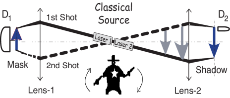
Figure 21: A ghost shadow can be made in coincidences by “blocking-unblocking” of the correlated laser beams, or simply by “blocking-unblocking” two correlated gun shots. The man-made trivial “correlation” of either laser beams or gun shots are deterministic, i.e., the laser beams or the bullets know where to go in each shot, which are fundamentally different from the quantum mechanical nontrivial nondeterministic multi-particle correlation.

A man-made factorizable correlation of laser beam is not only different from the non-factorizable correlations in type-one and type-two ghost imaging, but also different from the standard statistical correlation of intensity fluctuations. Although the experiment of Bennink et al. obtained a ghost shadow, which may be useful for certain purposes, it is clear that the physics shown in their experiment is fundamentally different from that of ghost imaging. In fact, this experiment can be considered as a good example to distinguish a man-made trivial deterministic classical intensity-intensity correlation from quantum entanglement and from a natural nonlocal nondeterministic multi-particle correlation.

(II) Correlated speckles.

Following a similar philosophy, Gatti et al. proposed a factorizable “speckle-speckle” classical correlation between two distant planes, $\vec{\rho}_{1}$ and $\vec{\rho}_{2}$, by imaging the speckles of the common light source onto the distant planes of $\vec{\rho}_{1}$ and $\vec{\rho}_{2}$, [13]

$$G^{(2)}(\vec{\rho}_{1},\vec{\rho}_{2})\propto\delta(\vec{\rho}_{o}-\vec{\rho}_{1}/m)\delta(\vec{\rho}_{o}-\vec{\rho}_{2}/m),$$ (67)

where $\vec{\rho}_{0}$ is the transverse coordinate in the plane of the light source.

The schematic setup of the classical simulation of Gatti et al. is depicted in Fig. 22 [13]. Their experiment used either entangled photon pairs of spontaneous parametric down-conversion (SPDC) or chaotic light for obtaining ghost shadows in coincidences.

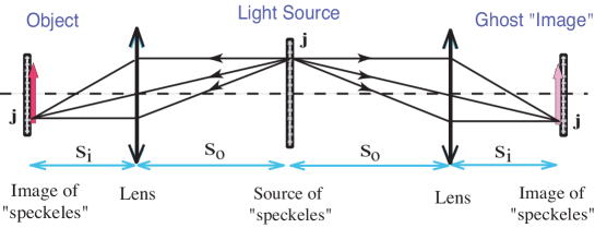
Figure 22: A ghost “imager” is made by blocking-unblocking the correlated speckles. The two identical sets of speckles on the object plane and the image plane, respectively, are the classical images of the speckles of the source plane. The lens, which may be part of a CCD camera used for the joint measurement, reconstructs classical images of the speckles of the source onto the object plane and the image plane, respectively. $s_{o}$ and $s_{i}$ satisfy the Gaussian thin lens equation $1/s_{o}+1/s_{i}=1/f$.

To distinguish from ghost imaging, Gatti et al. named their work “ghost imager”. The “ghost imager” comes from a man-made classical speckle-speckle correlation. The speckles observed on the object and image planes are the classical images of the speckles of the radiation source, reconstructed by the imaging lenses shown in the figure (the imaging lens may be part of a CCD camera used for the joint measurement). Each speckle on the source, such as the $j$th speckle near the top of the source, has two identical images on the object plane and on the image plane. Different from the non-factorizeable nonlocal image-forming correlation in type-one and type-two ghost imaging, mathematically, the speckle-speckle correlation is factorizeable into a product of two classical images of speckles. If two point photodetectors $D_{1}$ and $D_{2}$ are scanned on the object plane and the image plane, respectively, $D_{1}$ and $D_{2}$ will have more “coincidences” when they are in the position within the two identical speckles, such as the two $j$th speckles near the bottom of the object plane and the image plane. The blocking-unblocking of the speckles on the object plane by a mask will project a ghost shadow of the mask in the coincidences of $D_{1}$ and $D_{2}$. It is easy to see that the size of the identical speckles determines the spatial resolution of the ghost shadow. This observation has been confirmed by quite a few experimental demonstrations. There is no surprise that Gatti et al. consider ghost imaging classical [27]. Their speckle-speckle correlation is a man-made classical correlation and their ghost imager is indeed classical. The classical simulation of Gatti et al. might be useful for certain applications, however, to claim the nature of ghost imaging in general as classical, perhaps, is too far [27]. The man-made factorizable speckle-speckle correlation of Gatti et al. is a classical simulation of the natural nonlocal point-to-point image-forming correlation of ghost imaging, despite the use of either entangled photon source or classical light.

6 Local? Nonlocal?

We have discussed the physics of both type-one and type-two ghost imaging. Although different radiation sources are used for different cases, these two types of experiments demonstrated a similar non-factorizable point-to-point image-forming correlation:

Type-one:

$$\delta(\vec{\rho}_{1}-\vec{\rho}_{2})\sim\Big{|}\int d\vec{\kappa}_{s}\,d\vec{\kappa}_{i}\,\delta(\vec{\kappa}_{s}+\vec{\kappa}_{i})\,g_{1}(\vec{\kappa}_{s},\vec{\rho}_{1})\,g_{2}(\vec{\kappa}_{i},\vec{\rho}_{2})\Big{|}^{2},$$ (68)

Type-two:

$$1+\delta(\vec{\rho}_{1}-\vec{\rho}_{2}) \propto\langle\,\sum_{j}\sum_{l}\,\big{|}\frac{1}{\sqrt{2}}\big{[}E_{j}(\vec{\rho}_{1})E_{l}(\vec{\rho}_{2})+E_{l}(\vec{\rho}_{1})E_{j}(\vec{\rho}_{2})\big{]}\big{|}^{2}\,\rangle$$ (69)

$$=\langle\int d\vec{\kappa}\,d\vec{\kappa}^{\prime}\big{|}\frac{1}{\sqrt{2}}\big{[}g_{1}(\vec{\kappa},\vec{\rho}_{1})g_{2}(\vec{\kappa}^{\prime},\vec{\rho}_{2})+g_{2}(\vec{\kappa},\vec{\rho}_{2})g_{1}(\vec{\kappa}^{\prime},\vec{\rho}_{1})\big{]}\big{|}^{2}\rangle.$$

Equations (68) and (69) indicate that the point-to-point correlation of ghost imaging, either type-one or type-two, is the results of two-photon interference. Unfortunately, neither of them is in the form of $|\sum_{j}E_{j}|^{2}$ or $|E_{1}+E_{2}|^{2}$, and neither is measured at a local space-time point. The interference shown in Eqs. (68) and (69) occurs at different space-time points through the measurements of two spatially separated independent photodetectors.

In type-one ghost imaging, the $\delta$-function in Eq. (68) means a typical EPR position-position correlation of an entangled photon pair. In EPR’s language: when the pair is generated at the source the momentum and position of neither photon is determined, and neither photon-one nor photon-two “knows” where to go. However, if one of them is observed at a point at the object plane the other one must be found at a unique point in the image plane. In type-two ghost imaging, although the position-position determination in Eq. (69) is only partial, it generates more surprises because of the chaotic nature of the radiation source. Photon-one and photon-two, emitted from a thermal source, are completely random and independent, i.e., both propagate freely to any direction and may arrive at any position in the object and image planes. Analogous to EPR’s language: when the measured two photons were emitted from the thermal source, neither the momentum nor the position of any photon is determined. However, if one of them is observed at a point on the object plane the other one must have twice large probability to be found at a unique point in the image plane. Where does this partial correlation come from? If one insists on the view point of intensity fluctuation correlation, then, it is reasonable to ask why the intensities of the two light beams exhibit fluctuation correlations at $\vec{\rho}_{1}=\vec{\rho}_{2}$ only? Recall that in the experiment of Sarcelli et al. the ghost image is measured in the near-field. Regardless of position, $D_{1}$ and $D_{2}$ receive light from all (a large number) point sub-sources of the thermal source, and all sub-sources fluctuate randomly and independently. If $\Delta I_{1}\Delta I_{2}=0$ for $\vec{\rho}_{1}\neq\vec{\rho}_{2}$, what is the physics to cause $\Delta I_{1}\Delta I_{2}\neq 0$ at $\vec{\rho}_{1}=\vec{\rho}_{2}$?

The classical superposition is considered “local”. The Maxwell electromagnetic field theory requires the superposition of the electromagnetic fields, either $|\sum_{j}E_{j}|^{2}$ or $|E_{1}+E_{2}|^{2}$, takes place at a local space-time point $(\mathbf{r},t)$. However, the superposition shown in Eqs. (68) and (69) happens at two different space-time points $(\mathbf{r}_{1},t_{1})$ and $(\mathbf{r}_{2},t_{2})$ and is measured by two independent photodetectors. Experimentally, it is not difficult to make the two photo-detection events space-like separated events. Following the definition given by EPR-Bell, we consider the superposition appearing in Eqs. (68) and (69) nonlocal. Although the two-photon interference of thermal light can be written and calculated in terms of a semiclassical model, the nonlocal superposition appearing in Eq. (69) has no counterpart in the classical measurement theory of light, unless one forces a nonlocal classical theory by allowing the superposition to occur at a distance through the measurement of independent photodetectors, as we have done in Eq. (4.3). Perhaps, it would be more difficult to accept a nonlocal classical measurement theory of thermal light rather than to apply a quantum mechanical concept to “classical” thermal radiation.

Conclusion: In summary, we may conclude that ghost imaging is the result of quantum interference. Either type-one or type-two, ghost imaging is characterized by a non-factorizable point-to-point image-forming correlation which is caused by constructive-destructive interferences involving the nonlocal superposition of two-photon amplitudes, a nonclassical entity corresponding to different yet indistinguishable alternative ways of producing a joint photo-detection event. The interference happens within a pair of photons and at two spatially separated coordinates. The multi-photon interference nature of ghost imaging determines its peculiar features: (1) it is nonlocal; (2) its imaging resolution differs from that of classical; and (3) the type-two ghost image is turbulence-free. Taking advantage of its quantum interference nature, a ghost imaging system may turn a local “bucket” sensor into a nonlocal imaging camera with classically unachievable imaging resolution. For instance, using the Sun as light source for type-two ghost imaging, we may achieve an imaging spatial resolution equivalent to that of a classical imaging system with a lens of 92-meter diameter when taking pictures at 10 kilometers. Furthermore, any phase disturbance in the optical path has no influence on the ghost image. To achieve these features the realization of multi-photon interference is necessary.

Acknowledgment: The author thanks M. D’Angelo, G. Scarcelli, J.M. Wen, T.B. Pittman, M.H. Rubin, and L.A. Wu for helpful discussions. This work is partially supported by AFOSR and ARO-MURI program.

Appendix: Fresnel free-propagation

We are interested in knowing how a known field $E(\mathbf{r}_{0},t_{0})$ on the plane $z_{0}=0$ propagates or diffracts into $E(\mathbf{r},t)$ on another plane $z=$ constant. We assume the field $E(\mathbf{r}_{0},t_{0})$ is excited by an arbitrary source, either point-like or spatially extended. The observation plane of $z=$ constant is located at an arbitrary distance from plane $z_{0}=0$, either far-field or near-field. Our goal is to find out a general solution $E(\mathbf{r},t)$, or $I(\mathbf{r},t)$, on the observation plane, based on our knowledge of $E(\mathbf{r}_{0},t_{0})$ and the laws of the Maxwell electromagnetic wave theory. It is not easy to find such a general solution. However, the use of the Green’s function or the field transfer function, which describes the propagation of each mode from the plane of $z_{0}=0$ to the observation plane of $z=$ constant, makes this goal formally achievable.

Unless $E(\mathbf{r}_{0},t_{0})$ is a non-analytic function in the space-time region of interest, there must exist a Fourier integral representation for $E(\mathbf{r}_{0},t_{0})$

$$E(\mathbf{r}_{0},t_{0})=\int d\mathbf{k}\,E(\mathbf{k})\,w_{\mathbf{k}}(\mathbf{r}_{0},t_{0})\,e^{-i\omega t_{0}}, A-$$ (1)

where $w_{\mathbf{k}}(\mathbf{r}_{0},t_{0})$ is a solution of the Helmholtz wave equation under appropriate boundary conditions. The solution of the Maxwell wave equation $w_{\mathbf{k}}(\mathbf{r}_{0},t_{0})\,e^{-i\omega t_{0}}$, namely the Fourier mode, can be a set of plane-waves or spherical-waves depending on the chosen boundary condition. In Eq. ($A-$1), $E(\mathbf{k})=a(\mathbf{k})e^{i\varphi(\mathbf{k})}$ is the complex amplitude of the Fourier mode $\mathbf{k}$. In principle we should be able to find an appropriate Green’s function which propagates each mode under the Fourier integral point by point from the plane of $z_{0}=0$ to the plane of observation,

$$E(\mathbf{r},t) =\int d\mathbf{k}\,E(\mathbf{k})\,g(\mathbf{k},\mathbf{r}-\mathbf{r}_{0},t-t_{0})\,w_{\mathbf{k}}(\mathbf{r}_{0},t_{0})\,e^{-i\omega t_{0}}$$

$$=\int d\mathbf{k}\,g({\bf k},{\bf r}-{\bf r}_{0},t-t_{0})\,E({\bf k},{\bf r}_{0},t_{0}), A-$$ (2)

where $E({\bf k},{\bf r}_{0},t_{0})=E(\mathbf{k})\,w_{\mathbf{k}}(\mathbf{r}_{0},t_{0})\,e^{-i\omega t_{0}}$. The secondary wavelets that originated from each point on the plane of $z_{0}=0$ are then superposed coherently on each point on the observation plane with their after-propagation amplitudes and phases. It is convenient to write Eq. (Appendix: Fresnel free-propagation) in the following form

$$E(\vec{\rho},z,t)=\int d\omega\,d\vec{\kappa}\,g(\vec{\kappa},\omega;\vec{\rho}-\vec{\rho}_{0},z-z_{0},t-t_{0})\,E(\vec{\kappa},\omega;\vec{\rho}_{0},z_{0},t_{0}), A-$$ (3)

where we have used the transverse-longitudinal coordinates in space-time ($\vec{\rho}$ and $z$) and in momentum ($\vec{\kappa}$, $\omega$).

Fig. $A-$1 is a simple example in which the field propagates freely from an aperture $A$ of finite size on the plane $\sigma_{0}$ to the observation plane $\sigma$. Based on Fig. $A-$1 we evaluate $g(\vec{\kappa},\omega;\vec{\rho},z)$, namely the Green’s function for free-space Fresnel propagation-diffraction.

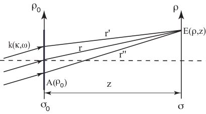
Figure $A-$1: Schematic of free-space Fresnel propagation. The complex amplitude $\tilde{A}(\vec{\rho}_{0})$ is composed of a real function $A(\vec{\rho}_{0})$ and a phase $e^{-i\vec{\kappa}\cdot\vec{\rho}_{0}}$ associated with each of the transverse wavevectors $\vec{\kappa}$ in the plane of $\sigma_{0}$. Notice: only one mode of wavevector $\mathbf{k}(\vec{\kappa},\omega)$ is shown in the figure.

According to the Huygens-Fresnel principle the field at a given space-time point $(\vec{\rho},z,t)$ is the result of a superposition of the spherical secondary wavelets that originated from each point on the $\sigma_{0}$ plane (see Fig. $A-$1),

$$E(\vec{\rho},z,t)=\int d\omega\,d\vec{\kappa}\ E(\vec{\kappa},\omega;0,0)\int_{\sigma_{0}}\,d\vec{\rho}_{0}\,\frac{\tilde{A}(\vec{\rho}_{0})}{r}\,e^{-i(\omega t-kr)}, A-$$ (4)

where we have set $z_{0}=0$ and $t_{0}=0$ at plane $\sigma_{0}$, and defined $r=\sqrt{z^{2}+|\vec{\rho}-\vec{\rho}_{0}|^{2}}$. In Eq. ($A-$4), $\tilde{A}(\vec{\rho}_{0})$ is the complex amplitude or relative distribution of the field on the plane of $\sigma_{0}$, which may be written as a simple aperture function in terms of the transverse coordinate $\vec{\rho}_{0}$, as we have done in the earlier discussions.

In the near-field Fresnel paraxial approximation, when $|\vec{\rho}-\vec{\rho}_{0}|^{2}\ll z^{2}$ we take the first-order expansion of $r$ in terms of $z$ and $\vec{\rho}$,

$$r=\sqrt{z^{2}+|\vec{\rho}-\vec{\rho}_{0}|^{2}}\simeq z(1+\frac{|\vec{\rho}-\vec{\rho}_{0}|^{2}}{2z^{2}}), A-$$ (5)

so that $E(\vec{\rho},z,t)$ can be approximated as

$$E(\vec{\rho},z,t)\simeq\int d\omega\,d\vec{\kappa}\ E(\vec{\kappa},\omega,0,0)\int d\vec{\rho}_{0}\,\frac{\tilde{A}(\vec{\rho}_{0})}{z}\,e^{i\frac{\omega}{c}z}\,e^{i\frac{\omega}{2cz}|\vec{\rho}-\vec{\rho}_{0}|^{2}}e^{-i\omega t},$$

where $e^{i\frac{\omega}{2cz}|\vec{\rho}-\vec{\rho}_{0}|^{2}}$ is named the Fresnel phase factor.

Assuming that the complex amplitude $\tilde{A}(\vec{\rho}_{0})$ is composed of a real function $A(\vec{\rho}_{0})$ and a phase $e^{-i\vec{\kappa}\cdot\vec{\rho}_{0}}$, associated with the transverse wavevector and the transverse coordinate on the plane of $\sigma_{0}$, as is reasonable for the setup of Fig. $A-$1, we can then write $E(\vec{\rho},z,t)$ in the form

$$E(\vec{\rho},z,t)=\int d\omega\,d\vec{\kappa}\ E(\vec{\kappa},\omega;0,0)\,e^{-i\omega t}\,\frac{e^{i\frac{\omega}{c}z}}{z}\int d\vec{\rho}_{0}\,A(\vec{\rho}_{0})\,e^{i\vec{\kappa}\cdot\vec{\rho}_{0}}\,e^{i\frac{\omega}{2cz}|\vec{\rho}-\vec{\rho}_{0}|^{2}}.$$

The Green’s function $g(\vec{\kappa},\omega;\vec{\rho},z)$ for free-space Fresnel propagation is thus

$$g(\vec{\kappa},\omega;\vec{\rho},z)=\frac{e^{i\frac{\omega}{c}z}}{z}\int_{\sigma_{0}}\,d\vec{\rho}_{0}\,A(\vec{\rho}_{0})\,e^{i\vec{\kappa}\cdot\vec{\rho}_{0}}\,G(|\vec{\rho}-\vec{\rho}_{0}|,\frac{\omega}{cz}). A-$$ (6)

In Eq. ($A-$6) we have defined a Gaussian function $G(|\vec{\alpha|},\beta)=e^{i(\beta/2)|\alpha|^{2}}$, namely the Fresnel phase factor. It is straightforward to find that the Gaussian function $G(|\vec{\alpha|},\beta)$ has the following properties:

$$G^{*}(|\vec{\alpha}|,\beta) = G(|\vec{\alpha}|,-\beta),$$

$$G(|\vec{\alpha}|,\beta_{1}+\beta_{2}) = G(|\vec{\alpha}|,\beta_{1})\,G(|\vec{\alpha}|,\beta_{2}),$$

$$G(|\vec{\alpha}_{1}+\vec{\alpha}_{2}|,\beta) = G(|\vec{\alpha}_{1}|,\beta)\,G(|\vec{\alpha}_{2}|,\beta)\,e^{i\beta\vec{\alpha}_{1}\cdot\vec{\alpha}_{2}},$$

$$\int d\vec{\alpha}\,\,G(|\vec{\alpha}|,\beta)\,e^{i\vec{\gamma}\cdot\vec{\alpha}} = i\frac{2\pi}{\beta}\,G(|\vec{\gamma}|,-\frac{1}{\beta}). A-$$ (7)

Notice that the last equation in Eq. (Appendix: Fresnel free-propagation) is the Fourier transform of the $G(|\vec{\alpha|},\beta)$ function. As we shall see in the following, these properties are very useful in simplifying the calculations of the Green’s functions $g(\vec{\kappa},\omega;\vec{\rho},z)$.

Next, we consider inserting an imaginary plane $\sigma^{\prime}$ between $\sigma_{0}$ and $\sigma$. This is equivalent to having two consecutive Fresnel propagations with a diffraction-free $\sigma^{\prime}$ plane of infinity. Thus, the calculation of these consecutive Fresnel propagations should yield the same Green’s function as that of the above direct Fresnel propagation shown in Eq. ($A-$6):

$$g(\omega,\vec{\kappa};\vec{\rho},z) A-$$ (8)

$$= C^{2}\frac{e^{i\frac{\omega}{c}(d_{1}+d_{2})}}{d_{1}d_{2}}\int_{\sigma^{\prime}}d\vec{\rho^{\prime}}\int_{\sigma_{0}}d\vec{\rho}_{0}\,\tilde{A}(\vec{\rho}_{0})G(|\vec{\rho^{\prime}}-\vec{\rho}_{0}|,\frac{\omega}{cd_{1}})G(|\vec{\rho}-\vec{\rho^{\prime}}|,\frac{\omega}{cd_{2}})$$

$$= C\,\frac{e^{i\frac{\omega}{c}z}}{z}\int_{\sigma_{0}}\,d\vec{\rho}_{0}\,\tilde{A}(\vec{\rho}_{0})\,G(|\vec{\rho}-\vec{\rho}_{0}|,\frac{\omega}{cz})$$

where $C$ is a necessary normalization constant for a valid Eq. ($A-$8), and $z=d_{1}+d_{2}$. The double integral of $d\vec{\rho}_{0}$ and $d\vec{\rho^{\prime}}$ in Eq. ($A-$8) can be evaluated as

$$\int_{\sigma^{\prime}}d\vec{\rho^{\prime}}\int_{\sigma_{0}}d\vec{\rho}_{0}\,\tilde{A}(\vec{\rho}_{0})\,G(|\vec{\rho^{\prime}}-\vec{\rho}_{0}|,\frac{\omega}{cd_{1}})\,G(|\vec{\rho}-\vec{\rho^{\prime}}|,\frac{\omega}{cd_{2}})$$

$$= \int_{\sigma_{0}}d\vec{\rho}_{0}\,\tilde{A}(\vec{\rho}_{0})\,G(\vec{\rho}_{0},\frac{\omega}{cd_{1}})\,G(\vec{\rho},\frac{\omega}{cd_{2}})$$

$$\times\int_{\sigma^{\prime}}d\vec{\rho^{\prime}}\,G(\vec{\rho^{\prime}},\frac{\omega}{c}(\frac{1}{d_{1}}+\frac{1}{d_{2}}))\,e^{-i\frac{\omega}{c}(\frac{\vec{\rho}_{0}}{d_{1}}+\frac{\vec{\rho}}{d_{2}})\cdot\vec{\rho^{\prime}}}$$

$$= \frac{i2\pi c}{\omega}\frac{d_{1}d_{2}}{d_{1}+d_{2}}\int_{\sigma_{0}}d\vec{\rho}_{0}\,\tilde{A}(\vec{\rho}_{0})\,G(\vec{\rho}_{0},\frac{\omega}{cd_{1}})\,G(\vec{\rho},\frac{\omega}{cd_{2}})\,$$

$$\hskip 68.2866pt\times\ G(|\frac{\vec{\rho}_{0}}{d_{1}}+\frac{\vec{\rho}}{d_{2}}|,\frac{\omega}{c}(\frac{d_{1}d_{2}}{d_{1}+d_{2}}))$$

$$= \frac{i2\pi c}{\omega}\frac{d_{1}d_{2}}{d_{1}+d_{2}}\int_{\sigma_{0}}d\vec{\rho}_{0}\,\tilde{A}(\vec{\rho}_{0})\,G(|\vec{\rho}-\vec{\rho}_{0}|,\frac{\omega}{c(d_{1}+d_{2})})$$

where we have applied Eq. (Appendix: Fresnel free-propagation), and the integral of $d\vec{\rho^{\prime}}$ has been taken to infinity. Substituting this result into Eq. ($A-$8) we obtain

$$g(\vec{\kappa},\omega;\vec{\rho},z)$$

$$= C^{2}\,\frac{i2\pi c}{\omega}\frac{e^{i\frac{\omega}{c}(d_{1}+d_{2})}}{d_{1}+d_{2}}\int_{\sigma_{0}}d\vec{\rho}_{0}\,\tilde{A}(\vec{\rho}_{0})\,G(|\vec{\rho}-\vec{\rho}_{0}|,\frac{\omega}{c(d_{1}+d_{2})})$$

$$= C\,\frac{e^{i\frac{\omega}{c}z}}{z}\int_{\sigma_{0}}\,d\vec{\rho}_{0}\,\tilde{A}(\vec{\rho}_{0})\,G(|\vec{\rho}-\vec{\rho}_{0}|,\frac{\omega}{cz}).$$

Therefore, the normalization constant $C$ must take the value of $C=-i\omega/2\pi c.$ The normalized Green’s function for free-space Fresnel propagation is thus

$$g(\vec{\kappa},\omega;\vec{\rho},z)=\frac{-i\omega}{2\pi c}\ \frac{e^{i\frac{\omega}{c}z}}{z}\int_{\sigma_{0}}\,d\vec{\rho}_{0}\,\tilde{A}(\vec{\rho}_{0})\,G(|\vec{\rho}-\vec{\rho}_{0}|,\frac{\omega}{cz}). A-$$ (9)

References

- [1] T.B. Pittman, Y.H. Shih, D.V. Strekalov, and A.V. Sergienko, Phys. Rev. A 52, R3429 (1995).
- [2] D.N. Klyshko, Usp. Fiz. Nauk, 154, 133 (1988); Sov. Phys. Usp, 31, 74 (1988); Phys. Lett. A 132, 299 (1988).
- [3] A. Einstein, B. Podolsky, and N. Rosen, Phys. Rev. 35, 777 (1935).
- [4] D.V. Strekalov, A.V. Sergienko, D.N. Klyshko and Y.H. Shih, Phys. Rev. Lett. 74, 3600 (1995). Due to its nonlocal behavior, this experiment was named “ghost” interference by the physics community.
- [5] G. Scarcelli, V. Berardi, and Y.H. Shih, Phys. Rev. Lett. 96, 063602 (2006).
- [6] A. Valencia, G. Scarcelli, M. D’Angelo, and Y.H. Shih, Phys. Rev. Lett. 94, 063601 (2005).
- [7] G. Scarcelli, A. Valencia, and Y.H. Shih, Europhys. Lett. 68, 618 (2004).
- [8] R. Meyers, K.S. Deacon, and Y.H. Shih, Phys. Rev. A 77, 041801(2008).
- [9] Y.H. Shih, IEEE J. of Selected Topics in Quantum Electronics, 9, 1455 (2003).
- [10] R. Hanbury-Brown, and R.Q. Twiss, Nature, 177, 27 (1956); 178, 1046, (1956); 178, 1447 (1956).
- [11] R. Hanbury-Brown, Intensity Interferometer, Taylor and Francis Ltd, London, 1974.
- [12] M.O. Scully and M.S. Zubairy, Quantum Optics, Cambridge University Press, Cambridge, 1997.
- [13] A. Gatti, E. Brambilla, M. Bache and L.A. Lugiato, Phys. Rev. A 70, 013802, (2004), and Phys. Rev. Lett. 93, 093602 (2004).
- [14] K. Wang, D. Cao, quant-ph/0404078; D. Cao, J. Xiong, and K. Wang, quant-ph/0407065.
- [15] Y.J. Cai, and S.Y. Zhu, quant-ph/0407240, Phys. Rev. E, 71, 056607 (2005).
- [16] B.I. Erkmen and J.H. Shapiro, Phys. Rev. A 77, 043809 (2008).
- [17] M. H. Rubin, Phys. Rev. A 54, 5349 (1996).
- [18] J. W. Goodman, Introduction to Fourier Optics, McGraw-Hill Publishing Company, New York, NY, 1968.
- [19] D.N. Klyshko, Photon and Nonlinear Optics, Gordon and Breach Science, New York, 1988.
- [20] R.J. Glauber, Phys. Rev. 130, 2529 (1963); Phys. Rev. 131, 2766 (1963).
- [21] M. D’Angelo, A. Valencia, M.H. Rubin, and Y.H. Shih, Phys. Rev. A 72, 013810 (2005).
- [22] J.C. Howell et al., Phys. Rev. Lett., 92, 210403 (2004).
- [23] W. Martienssen and E. Spiller, Am. J. Phys. 32, 919 (1964).
- [24] R. Meyers, K.S. Deacon, and Y.H. Shih, to be published.
- [25] J.B. Liu, and Y.H. Shih, Phys. Rev. A, 79, 023818 (2009).
- [26] R.S. Bennink, S.J. Bentley, and R.W. Boyd, Phys. Rev. Lett. 89, 113601 (2002); R.S. Bennink, et al., Phys. Rev. Lett. 92, 033601 (2004).
- [27] A. Gatti et al., Phys. Rev. Lett. 98, 039301 (2007) (comment); G. Scarcelli, V. Berardi, and Y.H. Shih, Phys. Rev. Lett. 98, 039302 (2007) (reply).