Part I 0

B. DASGUPTA    DASTGEERSHAIKH    Q. HUand G.P.ZANK Institute of Geophysics and Planetary Physics (IGPP),
University of California, Riverside, CA 92521. USA.
Email:dastgeer@ucr.edu

I–References

Minimum Dissipative Relaxed States Applied to Laboratory and Space Plasmas

B. DASGUPTA    DASTGEERSHAIKH    Q. HUand G.P.ZANK Institute of Geophysics and Planetary Physics (IGPP),
University of California, Riverside, CA 92521. USA.
Email:dastgeer@ucr.edu

Abstract

The usual theory of plasma relaxation, based on the selective decay of magnetic energy over the (global) magnetic helicity, predicts a force-free state for a plasma. Such a force-free state is inadequate to describe most realistic plasma systems occurring in laboratory and space plasmas as it produces a zero pressure gradient and cannot couple magnetic fields with flow. A different theory of relaxation has been proposed by many authors, based on a well-known principle of irreversible thermodynamics, the principle of minimum entropy production rate which is equivalent to the minimum dissipation rate (MDR) of energy. We demonstrate the applicability of minimum dissipative relaxed states to various self-organized systems of magnetically confined plasma in the laboratory and in the astrophysical context. Such relaxed states are shown to produce a number of basic characteristics of laboratory plasma confinement systems and solar arcade structure.

1 Introduction and Motivation:

Self-organization is a natural process [Ortolani and Schnack, 1993] in which a continuous system evolves toward some preferred states showing a form of order on long scales. Examples of such self-organization processes are ubiquitous in nature and in systems studied in the laboratory. These ordered states are very often remarkably robust, and their detailed structures are mostly independent of the way the system is prepared. The final state to which a system evolves generally depends on the boundary conditions, inherent geometry of the particular device, but is relatively independent of the initial conditions. Self-organization in plasma is generally called Plasma Relaxation. The seminal theory for plasma relaxation first proposed by Taylor (1974) yields a force-free state with zero pressure gradient. Taylor’s theory was the first to explain the experimentally observed field reversal of the Reversed Field Pinch (RFP).

Self-organized states with zero pressure gradient are often far from experimentally realizable scenarios. Any realistic magnetic configuration confining plasma must have a non-zero pressure gradient. Extensive numerical simulations [ Sato et al., 1996, Zhu et al., 1995] have established the existence of self-organized states of plasma with finite pressure, i.e., these states are observed to be governed by the magnetohydrodynamic force balance equation. Numerical simulations [Dasgupta et al, 1995, Watanabe et al, 1997] and experiments [Ono et al., 1993 ] have established that counterhelicity merging of two spheromaks can produce a Field-Reversed Configuration (FRC). The FRC has a zero toroidal magnetic field, and the plasma is confined entirely by poloidal magnetic field. It has a finite pressure, nonzero perpendicular component of current and is more often characterized by a high value of plasma beta. The stability and long life categorize FRC as a relaxed state, which is not obtainable from Taylor model of relaxation. Since spheromaks are depicted as a Taylor state [Rosenbluth and Bussac, 1979], formation of a FRC from the merging of two counterhelicity spheromaks is a unique process from the point of view of plasma relaxation, where a non-force free state (hence non-Taylor state) emerges from the coalescence of two Taylor states. In astrophysical context, particularly solar physics scenario, a 3-D MHD simulation by Amari and Luciano [2000], among others, showed that, after the initial helicity drive, the final “relaxed state is far from the … linear force-free model that would be predicted by Taylor’s conjecture” and they suggested to derive an alternative variational approach. Such physical processes call for an alternate model for plasma relaxation to broadly accommodate a large number of these observations.

In this context, an important work by Turner deserves special attention. Turner first showed (1986) that a relaxed magnetic field configuration which can support/confine a plasma with a finite pressure gradient. Adopting a two-fluid approach, a model of magnetofluid relaxation is constructed for Hall MHD, under the assumptions of minimum energy (magnetic plus fluid) with the constraints of global magnetic helicity hybrid helicity, axial magnetic flux and fluid vorticity. Euler-Lagrange equations resulted from such variational approach show the coupling between the magnetic field and the fluid vorticity. The solutions for such coupled equations are shown to be achieved by the linear superposition of the eigen-vectors of the ’curl’ operator (force-free states). These solutions yield magnetic field configurations which can confine plasma with a finite pressure gradient.

The principle of “minimum rate of entropy production” formulated by Prigogine and others [Prigogine, 1947] is believed to play a major role in many problems of irreversible thermodynamics. This principle states that for any steady irreversible processes, the rate of entropy production is minimum. For most irreversible processes in nature, the minimum rate of entropy production is equivalent to the minimum rate of energy dissipation. A magnetized plasma is such a dissipative system and it is appropriate to expect that the principle of minimum dissipation rate of energy has a major role to play in a magnetically confined plasma. It is worth mentioning that Rayleigh [1873] first used the term “principle of least dissipation of energy” in his works on the propagation of elastic waves in matter. Chandasekhar and Woltjer [1958] considered a relaxed state of plasma with minimum Ohmic dissipation with the constraint of constant magnetic energy and obtained an equation for the magnetic field involving a ‘double curl’ for the magnetic field and remarked that the solution of such equation is “much wider” than the usual force free solution.

Montgomery and Phillips [1988] first used the principle of minimum dissipation rate (MDR) of energy in an MHD problem to understand the steady the steady profile of a RFP under the constraint of a constant rate of supply and dissipation of helicity with the boundary conditions for a conducting wall. Farengo et al [Farengo et al, 1994,1995, 2002, Bouzat, 2006] in a series of papers applied the principle of MDR to a variety of problems ranging from flux-core spheromak to tokamak.

In this work, we present an alternative scenario for plasma relaxation which is based on the principle of minimum dissipation rate (MDR) rate of energy. This model gives us a non-force free magnetic field, capable of supporting finite pressure gradient. We demonstrate the this model can reproduce some of the basic characteristics of most of the plasma confining devices in the laboratory as well as the arcade structure of solar magnetic field. A two-fluid generalization of this model for an open system couples magnetic field with flow - so this model is applicable to other astrophysical situations.

The plan of the paper is as follows: In section 2, we present a single fluid MDR model for closed system and briefly discuss its applicarions to some of the laboratory plasma confinement devices, such as RFP, Spheromak, Tokamak and FRC. We present the result of a recent numerical simulation to justify our choice of the energy dissipation rate as an effective minimizer in our variation problem. In section 3 we describe a generalized version of the MDR model for open two fluid system and its application to solar arcade problem. We summarize a numerical extrapolation method for non-force free coronal magnetic field based on our MDR model. Section 4 concludes our paper.

2 Single fluid MDR based model

To obtain both the field reversal and a finite pressure gradient for RFP, Dasgupta et al.[ Dasgupta et al., 1998] considered the relaxation of a slightly resistive and turbulent plasma using the principle of MDR under the constraint of constant global helicity. With the global helicity $K_{M}$ and the dissipation rate $R$ defined as,

$$K_{M}=\int_{V}{\bf A}\cdot{\bf B}dV;\qquad R=\int_{V}\eta{\bf j}^{2}dV,$$ (1)

the variational principle $\delta(R-\Lambda K)$ leads to the following Euler-Lagrange equation,

$$\nabla\times\nabla\times\nabla\times{\bf B}=\Lambda{\bf B}.$$ (2)

Solutions of the above equation can be constructed as a superposition of the force free equation using Chandrasekhar-Kendall (CK) eigenfunctions [Chandraskhar and Kendall, 1957]

$$B=\alpha_{1}B_{1}+\alpha_{2}B_{2}+\alpha_{3}B_{3},$$ (3)

where $\alpha_{1},\alpha_{2},\alpha_{3}$ are constants, to be determined from the boundary conditions, and ${\bf B}_{i}^{\prime}s$ are obtained from

$$\nabla\times{\bf B}_{i}=\lambda_{i}B_{i};\quad(i=1,2,3);\quad\lambda_{i}^{3}=\Lambda.$$ (4)

We have used the analytic continuation of CK eigenfunctions in the complex domain. However, one can easily ascertain that the resulting magnetic field B is real. Moreover, since the superposition of force free fields with different eigenvalues $\lambda_{i}$ is not a force free field, the resultant magnetic field B is not force free, ${\bf J}\times{\bf B}\neq 0$. An explicit form of the solution in cylindrical geometry with the boundary conditions for an RFP (perfectly conducting wall) has shown two remarkable features: (1) Such a state can support a pressure gradient; and (2) Field reversal is found in states that are not force free.

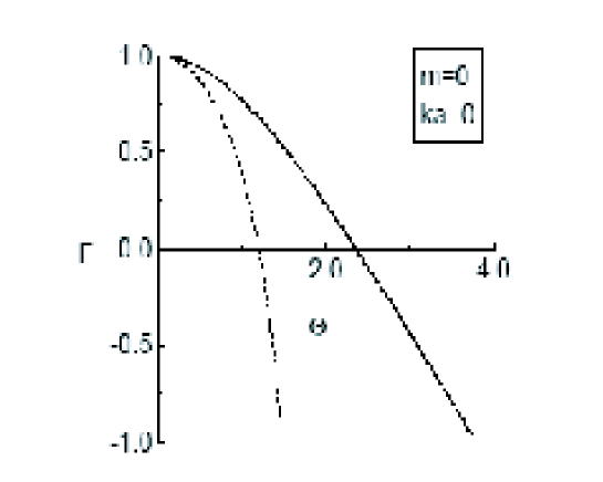
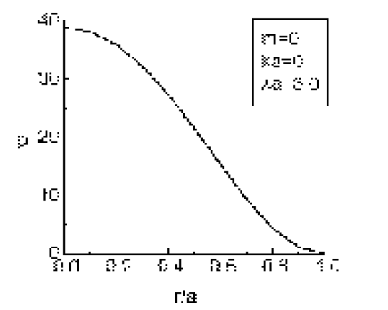
Figure 1: Left panel: Plot of $F=B_{z}(a)/\left<B_{z}\right>$ and $\Theta=B_{\theta}(a)/\left<B_{z}\right>$ ($<..>$ is the volume average and $a$ is the radial distance) showing the field reversal of RFP obtained from MDR model. The dotted curve represents the plot for the minimum energy state of Taylor. Right Panel: Pressure profile of RFP obtained from MDR model.(from Dasgupta et al., 1998).

In Figure 1 a plot of the field reversal parameter $F$ against the pinch parameter $\Theta$ is shown. It is found that axial field reverses at a value $\Theta\simeq 2.2$; and the pressure profile of the RFP obtained from our MDR model.

A success of this theory is its applicability in a tokamak configuration [Bhattacharya et al., 2000]. In toroidal geometry, the CK eigenfunctions are hypergeometric functions in the large aspect ratio approximation. Equilibria can be constructed under the assumption that the total current J = 0 at the edge. The solution reproduces the q-profile, the toroidal magnetic field, the pressure profile and $\sigma={\bf J}\cdot{\bf B}/B^{2}$ for tokamak, which are very close to the observed profiles (e.g., figure 2). The solutions allow for a tokamak, low-q discharge as well as RFP like behavior with a change of eigenvalue which would essentially determine the amount of volt-sec associated with the discharge characterizing the relaxed state. The poloidal Volt-sec/toroidal flux associated with the discharge can be directly interpreted in terms of the parameter $\lambda r_{0}$ ($r_{0}$ is the minor radius of the torus, $\lambda=\sqrt[3]{\Lambda}$) and can be shown to increase with $\lambda r_{0}$. MDR relaxed state can yield several kinds of solutions with distinct q-profiles. For low values of $\lambda r_{0}$, the q-profile is monotonically increasing and hence the solutions resemble a tokamak type discarge together with a nearly constant toroidal field, for larger values of $\lambda r_{0}$ the toroidal field reverses at the edge, signifying an RFP-type behavior and for intermediate values, the relaxed states indicate an ultra low-q type of discharge exhibiting a q-profile with a pitch minimum and $0<q<1$. In figure 2, we plot the toroidal magnetic field $B_{\phi},\sigma={\bf J}\cdot{\bf J}/B^{2},q$ and pressure profiles for different values of $\lambda r_{0}$, for a fixed value of the aspect ratio = 4.0. The continuous line corresponds corresponds to $\lambda r_{0}=1.5$, and shows a monotonic increase with $r$, which is the essential feature of tokamak discharge. For this case the the toroidal magnetic field ($B_{\phi}$) is essentially constant and the pressure profile has a peak at the center of the minor cross section of the torus and falls to zero at the edge. A non-constant behavior is shown by the $\sigma$ profile. The dotted line corresponds to $\lambda r_{0}=3.0$. In this case the toroidal field reverses sign at the edge, which corresponds to an RFP like discharge. The q-profile shows a similar behavior. The $\sigma$ profile has a dip at $r=0$ and exhibits a bump near the outer region. Such profiles have been experimentally observed in the ETA-BETA-II device [ Antoni et al, 1983]. For the values $\lambda r_{0}=2.5$ the q-profile shows a nonmonotonic behavior as shown in figure 3. The toroidal magnetic field again peaks at the center and slowly decreases towards the edge, showing a paramagnetic behavior that is typical of ultra low-q discharge [Yoshida et al., 1986]. Pressure profile peaks at the center and goes to zero at the edge. Some of these results have been observed in the SINP tokamak [Lahiri et al, 1996] and were also reported earlier in REPUTE-1 [Yoshida et al., 1986] and in TORIUT-6 [Yamada et al, 1987].

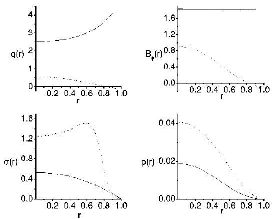
Figure 2: q-profile, $B_{\phi},\sigma$, and pressure profile of (i)Tokamak discharge (continuous line); (ii) RFP discharge (dotted line); (from Bhattacharya et al., 2000).

This model has been utilized to obtain the spheromak configuration from the spherically symmetric solution under appropriate boundary conditions relevant to an insulating boundary at the edge [Dasgupta et al., 2002]. These boundary conditions are are consistent with the classical spheromak solution used by Rosenbluth and Bussac [1979]. The most interesting part of this spheromak solution is the non-constant profile for ${\bf J}\cdot{\bf B}/B^{2}$ plotted against normalized distance from the magnetic axis. This profile shows peaks outside the magnetic axis, and this feature is qualitatively closer to the experimentally observed profile reported by Hart et al. [Hart et al., 1983].

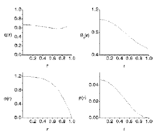
Figure 3: q-profile, $B_{\phi},\sigma$, and pressure profile of low-q Discharge; (from Bhattacharya et al., 2000).

The field-reversed configuration (FRC) is a compact toroidal confinement device [Tuszewski, 1988] which is formed with primarily poloidal magnetic field and a zero or negligibly small toroidal magnetic field. The plasma beta of the FRC is one of the highest for any magnetically confined plasma. FRC can be considered as a relaxed state [Guo et al, 2005, 2006], but it is a distinctly non-Taylor state. The FRC configuration can be obtained for an externally driven dissipative system which relaxes with minimum dissipation. In Bhattacharya et al., [2001] we show that the Euler-Lagrange equations for relaxation under MDR with magnetic energy as the constraint represents an FRC configuration for one choice of eigenvalues. This solution is characterized by high beta, zero helicity and a completely null toroidal field and supports a non-constant pressure profile (non-force free). Another choice of eigenvalue leads to a spheromak configuration. A generalization of this work incorporating flow [Bhattacharya et al., 2003] and taking magnetic and flow energies and cross helicities as constraints also produces the FRC configuration. This state supports field aligned flows with strong shears that may lead to stability and better confinement.

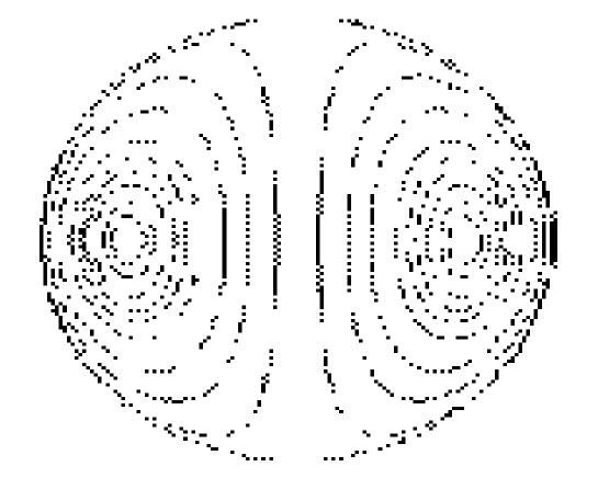
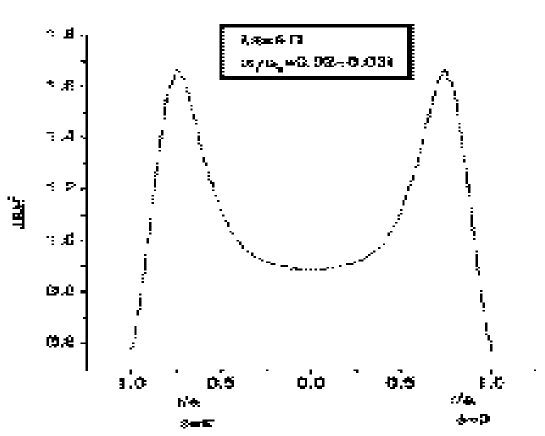
Figure 4: Spheromak configuration (left panel) and the non-constant $J_{||}/B$ derived from our model based on MDR (right panel); (from Dasgupta et al., 2002).

2.1 Simulation Results:

To justify the use of the MDR principle in plasma relaxation and the choice of the total dissipation rate as a minimizer in the variational principle we performed a fully 3-D numerical simulations for a turbulent and slightly dissipative plasma using a fully compressible MHD code [Shaikh et al., 2007] with periodic boundary conditions. Fluctuations are Fourier expanded and nonlinear terms are evaluated in real space. Spectral methods provide accurate representation in Fourier space. In our code there is very little numerical dissipation, and hence the ideal invariants are preserved. The selective decay processes (in addition to dissipation) depend critically on the cascade properties associated with the rugged MHD invariants that eventually govern the spectral transfer in the inertial range. This can be elucidated as follows [Biscamp, 2003]. Magnetic vector potential in 3D MHD dominates, over the magnetic field fluctuations, at the smaller Fourier modes, which in turn leads to a domination of the magnetic helicity invariant over the magnetic energy. On the other hand, dissipation occurs predominantly at the higher Fourier modes which give rise to a rapid damping of the energy dissipative quantity $R$. A heuristic argument for this process can be formulated in the following way. The decay rates of helicity $K$ and dissipation rate $R=\int_{V}\eta j^{2}dV$ in the dimensionless form, with the magnetic field Fourier decomposed as ${\bf B}({\bf k},t)=\Sigma_{k}{\bf b_{k}}\exp(i{\bf k}\cdot{\bf r})$, can be expressed as,

$$\frac{dK}{dt}=-\frac{2\eta}{S}\Sigma_{k}k{\bf b_{k}}^{2};\qquad\frac{dR}{dt}=-\frac{2\eta^{2}}{S^{2}}\Sigma_{k}k^{4}{\bf b_{k}}^{2}$$ (5)

where $S=\tau_{R}/\tau_{A}$, is the Lundquist number, $\tau_{R},\tau_{A}$ are the resistive and Alfvén time scales, respectively. The Lundquist number in our simulations varies between $10^{6}$ and $10^{7}$. We find that at scale lengths for which $k\approx S^{1/2}$, the decay rate of energy dissipation is $\sim O(1)$ . But at these scale lengths, helicity dissipation is only $\sim O(S^{-1/2})\ll 1$. This physical scenario is consistent with our 3D simulations. Figure 5 shows the time evolution of the global helicity $K_{M}$, total magnetic energy $W_{M}$ and the total dissipation rate $R$. It is seen that global helicity remains approximately constant, (decaying very slightly during the simulation time) while the magnetic energy decays faster than the global helicity, but the energy dissipation rate decays even faster than the magnetic energy. The results of the simulation show that total dissipation rate can serve as a minimizer during a relaxation process.

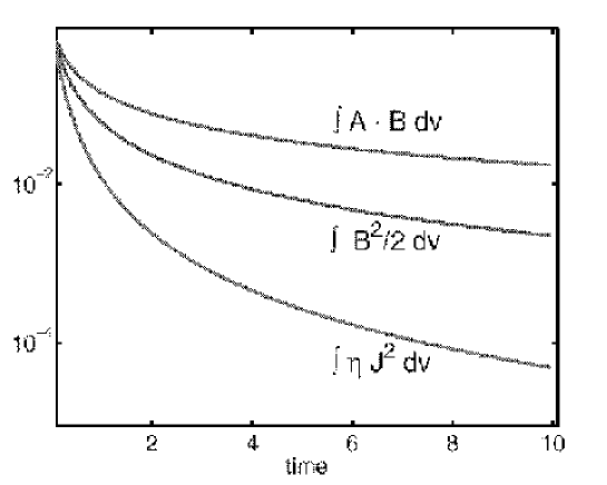
Figure 5: Time evolution of decay rates associated with the turbulent relaxation of the ideal MHD invariants, viz, global magnetic helicity $K_{M}=\int_{V}{\bf A}\cdot{\bf B}dV$, magnetic energy $W=\int_{V}B^{2}/2dV$ and the total dissipation $R=\int_{V}\eta J^{2}dV$, all shown in the same scale.

3 MDR based relaxation model for two fluid plasma with external drive:

Recently, Bhattacharya and Janaki [2004] developed a theory of dissipative relaxed states in two-fluid plasma with external drive. We describe the plasma (consisting of ions and electrons) by the two-fluid equations. The basic advantages of a two-fluid formalism over the single-fluid or MHD counterpart are: (i) in a two-fluid formalism, one can incorporate the coupling of plasma flow with the magnetic field in a natural way, and (ii) the two-fluid description being more general than MHD, is expected to capture certain results that are otherwise unattainable from a single-fluid description. It should be mentioned that although we are invoking the principle of minimum dissipation rate of energy - instead of the principle of minimum energy - our approach is closely similar to the approach to plasma relaxation including Hall terms, as developed by Turner (1986).

In the two-fluid formalism the canonical momentum ${\bf{P}}_{j}$ canonical vorticity ${\bf{\Omega}}_{j}$, for the $j$-th species are defined respectively as,

$${\bf{P}}_{j}=m_{j}{\bf{u}}_{j}+\frac{q_{j}}{c}{\bf{A}},\qquad{\bf{\Omega}}_{j}=\nabla\times{\bf{P}}_{j},\quad(j=i,e).$$ (6)

A gauge invariant expression for the generalized helicity is introduced by defining

$$K_{j}=\int_{V}{\bf{P}}_{j}\cdot{\bf{\Omega}}_{j}d\tau-\int_{V}{\bf{P}}_{j}^{\prime}\cdot{\bf{\Omega}}_{j}^{\prime}dV;$$ (7)

which is a relative helicity with respect to reference field having ${\bf{P}}_{j}^{\prime}$ as the canonical momentum, and ${\bf{P}}_{\alpha}$ and ${\bf{P}}_{\alpha}^{\prime}$ are different inside the volume of interest and the same outside. The gauge invariance condition holds

$$({\bf{\Omega}}_{j}-{\bf{\Omega}}_{j}^{\prime})\cdot\hat{n}=0\Rightarrow({\bf{B}}-{\bf{B}}^{\prime})\cdot\hat{n}=0\qquad({\bf{\omega}}_{j}-{\bf{\omega}}_{j}^{\prime})\cdot\hat{n}=0,\quad({\bf{\omega}}_{j}=\nabla\times{\bf{u}}_{j}),$$ (8)

under the condition that there is no flow-field coupling at the surface. The above equations then represent natural boundary conditions inherent to the problem.

The helicity balance equation for the generalized helicity, obtained from the balance equations for the generalized momentum and vorticity, consists of two terms, the helicity injection terms and helicity dissipation term (containing resistivity and viscosity). The global helicity can be taken as a bounded function following Montgomery et al.,(1988) and it is possible to form a variational problem with the helicity dissipation rates as constraints. Thus,

$$\frac{dK_{\alpha}}{dt} = -\oint[G_{\alpha}-{\bf{P}}_{\alpha}\cdot{\bf{u}}_{\alpha}]{\bf{\Omega}}_{\alpha}^{\prime}\cdot\hat{n}da-\oint({\bf{P}}_{\alpha}\cdot{\bf{\Omega}}_{\alpha}){\bf{u}}_{\alpha}\cdot\hat{n}da$$ (9)

$$- \oint\left(\frac{\partial{\bf{P}}_{\alpha}^{\prime}}{\partial t}\times{\bf{P}}_{\alpha}^{\prime}\right)\cdot\hat{n}da-\eta_{\alpha}^{\prime}\oint[\{\nabla\times{\bf{B}}+L_{\alpha}{\bf{\omega}}_{\alpha})\}\times{\bf{P}}_{\alpha}]\cdot\hat{n}da$$

$$- 2\eta_{\alpha}^{\prime}\int[\nabla\times({\bf{B}}+L_{\alpha}{\bf{\omega}}_{\alpha})]\cdot{\bf{\Omega}}_{\alpha}d\tau$$

with

$$G_{\alpha}=\left[q_{\alpha}\phi+\frac{h_{\alpha}}{n_{\alpha}}-\frac{m_{\alpha}u_{\alpha}^{2}}{2}\right];\qquad\eta_{\alpha}^{\prime}=\frac{q_{\alpha}\eta c}{4\pi}$$

$$L_{\alpha}=\frac{4\pi}{q_{\alpha}cn_{\alpha}}\frac{\mu_{\alpha}}{\eta}\equiv~{}~{}{\rm{Prandtl~{}~{}number.}}$$ (10)

The minimization integral is then obtained as,

$${\cal{I}} = \int\left[(\nabla\times{\bf{B}})\cdot(\nabla\times{\bf{B}})+\frac{4\pi nqL_{i}}{c}{\bf{\omega}}_{i}\cdot{\bf{\omega}}_{i}\right]d\tau$$ (11)

$$+ \lambda_{i}\int[\nabla\times({\bf{B}}+L_{i}{\bf{\omega}}_{i})]\cdot{\bf{\Omega_{i}}}d\tau-\lambda_{e}\int(\nabla\times{\bf{B}})\cdot{\bf{\Omega}}_{e}d\tau$$

where $L_{i}=4\pi\mu_{i}/ecn_{i}\eta$ is the magnetic Prandtl number for ions, $\mu_{i}$ is the ion viscosity and $\eta$ is the resistivity. We assumed the electron mass $m_{e}\rightarrow 0.$ The first two terms in the above integral represent the ohmic and viscous dissipation rates while the second two integrals represent the ion and electron generalized helicity dissipation rates. $\lambda_{i}$ and $\lambda_{e}$ are the corresponding Lagrange undetermined multipliers.The Euler-Lagrange equations are written as,

$$\nabla\times\nabla\times{\bf{B}}+\frac{(\lambda_{i}+\lambda_{e})q}{c}\nabla\times){\bf{B}}+\frac{\lambda_{i}}{2}\left(\frac{qL_{i}}{c}+m_{i}\right)(\nabla\times){\bf{\omega}}_{i}=\nabla\psi;$$ (12)

$$\nabla\times\nabla\times{\bf{\omega}}_{i}+\frac{2\pi nq}{m_{i}\lambda_{i}c}\nabla\times{\bf{\omega}}_{i}+\frac{1}{2m_{i}L_{i}}\left(\frac{qL_{i}}{c}+m_{i}\right)(\nabla\times)^{2}{\bf{B}}=\nabla\chi;$$ (13)

where $\psi$ and $\chi$ are arbitrary gauge functions, with $\nabla^{2}\psi=\nabla^{\chi}=0$. Following Turner (1986) we can write the exact solution of the coupled equations (12) and (13) as a linear superposition of two CK eigenfunctions, which are the solutions of $\nabla\times{\bf{Y}}_{k}=\lambda_{k}{\bf{Y}}_{k}$ i.e.,

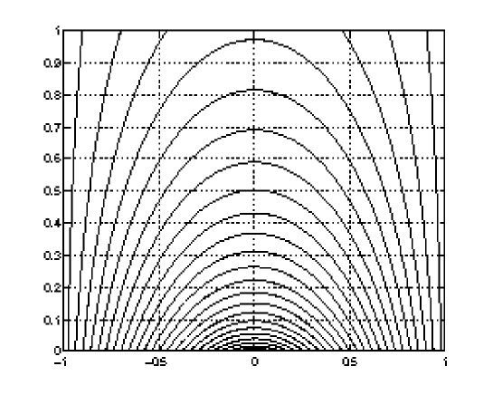
Figure 6: Flow lines in the $x$-$z$ plane for $\gamma=1.5$ (from Bhattacharya et al., 2007).

$${\bf{B}}={\bf{Y}}_{1}+\alpha{\bf{Y}}_{2}\qquad{\bf{\omega}}_{i}={\bf{Y}}_{1}+\beta{\bf{Y}}_{2},$$ (14)

and $\alpha$ and $\beta$ are constants and quantify the non force-free part, to be obtained from some boundary conditions.

3.1 Application to solar arcade problem

One of the important features of this formalism is the presence of a nontrivial flow and the coupling between the magnetic field and the flow. The solutions of the corresponding Euler-Lagrange equation highlight the role of nonzero plasma flow in securing a steady MDR relaxed state for an open and externally driven system. This model has been very successful in describing the arcade structures observed in Solar corona [Bhattacharya et al., 2007]. To model solar arcade-type magnetic fields, we make some simplified assumptions and consider a 2-D magnetic field in the $x$-$z$ plane with the $x$ direction lying on the photosphere surface and $z$ is the vertical direction. With appropriate boundary conditions and after some lengthy algebra, the solutions for the components of the magnetic fields are obtained as,

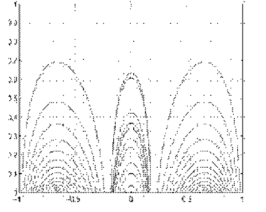
Figure 7: Magnetic field lines in the $x$-$z$ plane corresponding to (i) single arcade structure for $\gamma=1.5$ in left panel and (ii) triple arcade structure for $\gamma=3.36$ in right panel (from Bhattacharya et al., 2007).

$$B_{x}=\sqrt{\gamma^{2}-1}\left[2\cos\gamma x-\frac{2\cos\gamma}{\cos\sqrt{\gamma^{2}-1}}\cos(x\sqrt{\gamma^{2}-1})\right]e^{-z\sqrt{\gamma^{2}-1}};$$

$$B_{y}=0;$$ (15)

$$B_{z}=-\left[2\gamma\sin\gamma x-\frac{2\sqrt{\gamma^{2}-1}\cos\gamma}{\sin\sqrt{\gamma^{2}-1}}\sin(x\sqrt{\gamma^{2}-1})\right]e^{-z\sqrt{\gamma^{2}-1}};$$

with $\gamma=\sqrt{(k^{2}+\lambda^{2})/\lambda^{2}}$ ($\lambda$ is the eigenvalue and $k$ is the wave number associated with the solution). The same procedures can be adopted for the flow pattern. In figure 7 the magnetic field lines in the$x$-$z$ plane is plotted for two different values of the parameter $\gamma$. The arcade structures are obtained by solving the field line equations $\frac{dz}{dx}=\frac{B_{z}}{B_{x}}$. It is interesting to note that the arcade structure changes with the change of the single parameter $\gamma$. Figure 6 plots the flow lines for $\gamma=1.5$. In cylindrical geometry the solutions of eqn. (12) can be written in terms of a superposition of Bessel functions. Such solutions yield 3-D Flux ropes, which are plotted in the Figure (8).

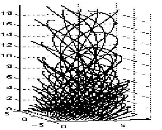
Figure 8: Plot of 3-D Fluxrope obtained from the solution eqn.(12).

3.2 Non-force Free Coronal Magnetic Field Extrapolation Based on MDR:

An outstanding problem in solar physics is to derive the coronal magnetic field structure from measured photospheric and/or chromospheric magnetograms. A new approach to deriving three-dimensional non-force free coronal magnetic field configurations from vector magnetograms, based on the MDR principle has been recently developed [Hu, Dasgupta, & Choudhary (2007)]. In contrast to the principle of minimum energy, which yields a linear force-free magnetic field, the MDR gives a more general non-force free magnetic field with flow. The full MDR-based approach requires two layers of vector magnetic field measurements. Its exact solution can be expressed as the superposition of two linear force-free fields with distinct $\lambda$ parameters, and one potential field. The final solution is thus decomposed into three linear force-free extrapolations, with bottom boundary conditions derived from the measured vector magnetograms, at both photospheric and chromospheric levels. The semi-analytic test case shown in Figure 9 illustrates the feasibility and the high performance of this method. This extrapolation is easy to implement and much faster than most other nonlinear force-free methods [Hu & Dasgupta 2007]. It also takes full advantage of multiple layer solar magnetic field measurements, thus gives a more realistic result.

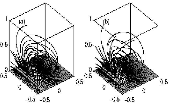
Figure 9: 3D view of magnetic field lines in a box simulating the typical extrapolation domain. (a) exact solution; (b) numerical extrapolation result. Bottom image at height 0 shows the normal field component distribution with gray scale indicating strongly negative (black) to positive (white) field. The great ressemblance between the exact and the numerical solutions justifies the feasibility and high performance of this method (Hu, Dasgupta, & Choudhary 2007).

4 Conclusion

We have demonstrated that a relaxation model based on the minimum dissipation of energy can successfully explain some of the salient observations both in laboratory and space plasma. An MDR based model model in its simpler form is capable of yielding basic characteristics of most of the laboratory plasma confinement devices, and a generalization of this model for two fluid with external drive can couple magnetic field and flow and predict solar arcade structures. The above findings definitely points out that the MDR relaxed states applied to astrophysical plasmas is a worthy case for further investigations. In future we plan to apply this model to investigate magnetic field structure in the sun with an aim to understanding coronal mass ejection.

5 Acknowledgement

We gratefully acknowledge partial supports from NASA LWS grant NNX07A073G, and NASA grants NNG04GF83G, NNG05GH38G, NNG05GM62G, a Cluster University of Delaware subcontract BART372159/SG, and NSF grants ATM0317509, and ATM0428880.

9

References

- [1] Amari, T., and Luciani, J. F., Phys. Rev. Letts., 84, 1196, (2000)
- [2] Antoni, V., S. Martini, S. Ortolini and R. Paccagnella, in Workshop on Mirror-based and Field-reversed approaches to Magnetic Fusion, Int. School of Plasma Physics, Varenna, Italy, p. 107, (1983)
- [3] Bhattacharya, R., M.S. Janaki and B. Dasgupta, Phys. Plasmas,7, 4801, (2000)
- [4] Bhattacharya, R., M.S. Janaki and B. Dasgupta, Phys. Lett. A , 291A, 291, (2001)
- [5] Bhattacharyya, R., M. S. Janaki and B. Dasgupta, Plasma Phys. Contr. Fusion, 45, 63 (2003).
- [6] Bhattacharya, R., and M. S. Janaki, Phys. Plasmas, 11, 5615 (2004)
- [7] Bhattacharya, R., M. S. Janaki, B. Dasgupta, G. P. Zank, Solar Phys. 240, 63, (2007)
- [8] Biskamp, D. 2003, Magnetohydrodynamic Turbulence, Cambridge University Press.
- [9] Bouzat, S. and R. Farengo, J. Plasma Phys., 72, 443, (2006)
- [10] Chandrasekhar, S. & P. C. Kendall, Astrophys. J., 126, 457 (1957).
- [11] Chandrasekhar, S. & L. Woltjer, Proc. Natl. Acad. Sci. USA, 44, 285 (1958).
- [12] Dasgupta, B., T. Sato, T Hayashi, K. Watanabe and T-H Watanabe, Trans. Fusion Tecnol., 27, 374, (1995)
- [13] Dasgupta, B., P. Dasgupta, M. S. Janaki, T. Watanabe and T. Sato, Phys. Rev. Lett., 81, 3144, (1998)
- [14] Dasgupta, B., M. S. Janaki, R. Bhattacharya, P. Dasgupta, T. Watanabe, and T. Sato, Phys. Rev. E , E 65, 046405, (2002)
- [15] Farengo, R. and J. R Sobehart, Plasma Phys. Contr. Fus., 36, 465 (1994)
- [16] Farengo, R. and J. R. Sobehart. Phys. Rev. E, 52, .2102 (1995)
- [17] Farengo, R. and K. I. Caputi, Plasma Phys. Contr. Fus., 44, 1707 (2002)
- [18] Guo, H. Y.., A. L. Hoffman, L. C. Steinhauer, and K. E. Miller, Phys. Rev. Letts, 95. 175001, (2005)
- [19] Guo, H. Y., A. L. Hoffman, L. C. Steinhauer, K. E. Miller, and R. D. Milroy, Phys. Rev. Letts, 97. 175001, (2006)
- [20] Hu, Q., Dasgupta, B., & Choudhary, D.P. 2007, AIP CP, 932, 376, (2007)
- [21] Hu, Q., and Dasgupta, B. , Sol. Phys., 247, 87, (2008)
- [22] Hart, G. W., C. Chin-Fatt, A. W. deSilva, G. C. Goldenbaum, R. Hess and R. S. Shaw, Phys. Rev. Lett., 51, 1558, (1983)
- [23] Lahiri, S., A. N. S. Iyenger, S. Mukhopadhyay and R. Pal, Nucl. Fusion, 36, 254, (1996)
- [24] Montgomery D. and L. Phillips, Phys. Rev. A, 38, 2953 (1988)
- [25] Ono, Y., A. Morita, and M. Katsurai and M Yamada, Phys. Fluids, B5, 3691, (1993)
- [26] Ortolani, S. and D. D. Schnack, Magnetohydrodynamics of plasma relaxation, World Scientific, (1993)
- [27] Prigogine, I., Etude Thermodynamique des Phénomènes Irreversibles, Editions Desoer, Liège, (1946)
- [28] Rayleigh, Proc. Math Soc. London, 363, 357 (1873)
- [29] Rosenbluth, M. N. and M. N. Bussac, Nucl. Fusion, 19, 489, (1979)
- [30] Sato, T. and Complexity Simulation Group: S. Bazdenkov, B.Dasgupta, S. Fujiwara, A. Kageyama, S. Kida, T. Hayashi, R. Horiuchi, H. Muira, H. Takamaru, Y. Todo, K. Watanabe and T.-H. Watanabe, Phys. Plasmas. 3, 2135 (1996)
- [31] Shaikh, D., B. Dasgupta, G. P., Zank, and Q. Hu, Phys. Plasmas, 15, 012306, (2008)
- [32] Taylor, J. B., Phys. Rev. Lett. 33, 139 (1974)
- [33] Turner, L., IEEE Trans. Plasma Sc. 14 , 849, (1986)
- [34] Tuszewski, M., Nuc. Fusion, 28, 2033, (1988)
- [35] Watanabe, T.-H., T. Sato, and T. Hayashi, Phys. Plasmas 4, (1997)
- [36] Yamada, H., K. Kusano, Y. Kamada, H. Utsumi, Z. Yoshida and N. Inoue, Nucl. Fusion, 27, 1169, (1987)
- [37] Yoshida, Z., S. Ishida, K. Hattori, Y. Murakami and J. Morikawa, J. Phys. Soc. Jpn., 55, 554, (1986)
- [38] Zhu, S., R. Horiuchi, and T. Sato, Phys. Rev. E, 51, 6047 (1995).