Horizons vs. singularities in spherically symmetric space-times

Abstract

We discuss different kinds of Killing horizons possible in static, spherically symmetric configurations and recently classified as “usual”, “naked” and “truly naked” ones depending on the near-horizon behavior of transverse tidal forces acting on an extended body. We obtain necessary conditions for the metric to be extensible beyond a horizon in terms of an arbitrary radial coordinate and show that all truly naked horizons, as well as many of those previously characterized as naked and even usual ones, do not admit an extension and therefore must be considered as singularities. Some examples are given, showing which kinds of matter are able to create specific space-times with different kinds of horizons, including truly naked ones. Among them are fluids with negative pressure and scalar fields with a particular behavior of the potential. We also discuss horizons and singularities in Kantowski-Sachs spherically symmetric cosmologies and present horizon regularity conditions in terms of an arbitrary time coordinate and proper (synchronous) time. It turns out that horizons of orders 2 and higher occur in infinite proper times in the past or future, but one-way communication with regions beyond such horizons is still possible.

I Introduction

As was pointed out by Horowitz and Ross HR1 ; HR2 , in some static black hole space-times, although all curvature invariants are everywhere finite, including the event horizon, an extended body falling into the black hole experiences enormous tidal forces in the immediate vicinity of the horizon. Large tidal forces emerge because in some cases the curvature components in a freely falling reference frame are significantly enhanced as compared with their static values. These objects were termed [1, 2] “naked black holes” because the behavior of tidal forces at the horizon resembles that near naked singularities. Examples of this behavior have been found in a wide class of theories of gravity including supergravities that arise in the low-energy limit of string theory.

Refs. ZP ; Z further classified such black holes and the corresponding event horizons as simply “naked” and “truly naked” ones: in the former, tidal forces experienced by a freely falling body are enhanced with respect to the static frame but remain finite. In the latter, the tidal forces become infinite. These properties depend on the asymptotic behavior of the curvature tensor near the horizon.

It should be noted that, despite the same physical idea behind the notion of a naked horizon in Refs. HR1 ; HR2 and ZP ; Z , the particular criteria are different. Namely, Refs. HR1 ; HR2 considered a number of examples of black hole solutions of dilaton gravity, supergravities etc. and showed that tidal forces near the horizon can become arbitrarily large as one approaches some (singular) limit in the parameter space of the corresponding solution, whereas the curvature invariants remain finite and become infinite only when the above limit is reached. The criterion used in ZP ; Z is more formal: a horizon is called naked if some quantity, characterizing the tidal forces at the horizon, is zero in the static reference frame but is finite and nonzero in a freely falling reference frame. (Such horizons, from the viewpoint of HR1 ; HR2 , may be characterized as “potentially naked” since the tidal forces can really become very large at some values of the solution parameters.) This definition is much more convenient for general studies and classification of horizons in different black hole solutions, and, using it, horizons in static, spherically symmetric black hole metrics were divided in ZP ; Z into three classes: usual, naked and truly naked. The classification was formulated in terms of the near-horizon behavior of the metric in the curvature (Schwarzschild-like) coordinates.

In the present paper, we study the extensibility of the metrics beyond horizons of different kinds. We show that the metric can be analytically (or at least sufficiently smoothly) extended under some stringent conditions which are explicitly written. All black hole metrics, for which the extensions are well-known, certainly satisfy these conditions. It turns out, however, that all “truly naked” horizons, as well as many of those previously characterized as naked and even usual ones, do not admit an extension and therefore must be considered as singularities. Indeed, timelike and null geodesic incompleteness is generally regarded as a criterion for the presence of a singularity (see, e.g., wald ), used, in particular, in the well-known singularity theorems. And it is precisely such incompleteness that takes place at inextensible horizons (sometimes also called “singular horizons”), despite finite values of the curvature invariants. Our approach is thus somewhat complementary to the discussion on singularities in black hole physics conducted in Refs. tipler ; pois ; brady ; nolan ; ori

It is natural to extend the consideration to the cosmological counterparts of static, spherically symmetric configurations, i.e., Kantowski-Sachs(KS) cosmological models. It can be mentioned that KS cosmologies are not excluded by modern observations if one assumes their sufficiently early isotropization craw , and the latter may follow from the process of matter creation from vacuum — see a discussion and some estimates in bd07 ; bz1 . It is also known bz1 that if the matter content of the Universe satisfies the Null Energy Condition, then the only way of avoiding a cosmological singularity in the past of a KS cosmology is the beginning of the cosmological evolution from a Killing horizon. Thus there is a good reason for studying the properties of such horizons, and some of them are described here.

The structure of the paper is as follows. Sec. II contains some general relations for spherically symmetric metrics, needed in the further study. Sec. III discusses the properties of the so-called quasiglobal coordinate as a convenient tool for studying the extensibility problem. In Sec. IV we obtain the horizon extensibility conditions in terms of an arbitrary radial coordinate and, using the curvature coordinate $r$, compare the extensibility criterion with the previously given ZP ; Z classification of horizons as usual, naked and truly naked ones in static, spherically symmetric space-times. Sec. V contains a number of examples showing which kinds of matter can create configurations with different kinds of horizons, including TNHs. In Sec. VI we discuss horizons in KS cosmologies and present the extensibility conditions in terms of an arbitrary time coordinate and proper (synchronous) time. Sec. VII contains some concluding remarks, in particular, on different kinds of singularities in spherically symmetric configurations of matter with negative pressure.

II Geometry

The general static, spherically symmetric metric can be written in the form

$$ds^{2}={\,\rm e}^{2\gamma(R)}dt^{2}-{\,\rm e}^{2\alpha(R)}dR^{2}-r^{2}(R)d\Omega^{2},\hskip 28.45274ptd\Omega^{2}\equiv d\theta^{2}+\sin^{2}\theta d\phi^{2},$$ (1)

where $R$ is an arbitrary radial coordinate. The most frequently used curvature (Schwarzschild) coordinate corresponds to the “gauge” condition $R\equiv r$. Another useful choice is the so-called quasiglobal radial coordinate $R=u$, corresponding to the “gauge” $g_{00}g_{11}=-1$, so that the metric is

$$ds^{2}=A(u)dt^{2}-\frac{du^{2}}{A(u)}-r^{2}(u)d\Omega^{2}.$$ (2)

The nonzero components of the Riemann tensor in the above two gauges are

$$R^{01}{}_{01} = -{{\displaystyle\frac{1}{2}}}A^{\prime\prime}=-{\,\rm e}^{-\alpha-\gamma}\left(\gamma_{r}{\,\rm e}^{\gamma-\alpha}\right)_{r}=-K_{1};$$

$${}R^{02}{}_{02} = -{{\displaystyle\frac{1}{2}}}\frac{A^{\prime}r^{\prime}}{r}=-{\,\rm e}^{-2\alpha}\frac{\gamma_{r}}{r}=-K_{2}=R^{03}{}_{03};$$

$${}R^{12}{}_{12} = -A\frac{r^{\prime\prime}}{r}-{{\displaystyle\frac{1}{2}}}\frac{A^{\prime}r^{\prime}}{r}={\,\rm e}^{-2\alpha}\frac{\alpha_{r}}{r}=-K_{3}=R^{13}{}_{13};$$

$${}R^{23}{}_{23} = \frac{1}{r^{2}}(1-Ar^{\prime}{}^{2})=\frac{1}{r^{2}}({\,\rm e}^{-2\alpha}-1)=-K_{4},$$ (3)

where expressions for the metric (2) are given in each line after the first equality sign and those for the curvature coordinates [Eq. (1) with $R\equiv r$] after the second equality sign. The prime stands for $d/du$ and the subscript $r$ for $d/dr$.

As follows from the geodesic deviation equations, the tidal forces experienced by bodies in the gravitational field (1) are conveniently characterized by the quantities Z

$$Z:=R^{12}{}_{12}-R^{02}{}_{02}=K_{2}-K_{3}$$ (4)

in the static reference frame and

$${\widetilde{Z}}\sim{\,\rm e}^{-2\gamma}Z=Z/A$$ (5)

in a freely falling reference frame near a horizon. These quantities have been used in Z to distinguish usual, naked and truly naked horizons.

Assuming $A<0$ in the metric (2), we obtain a Kantowski-Sachs (KS) spherically symmetric cosmology in which $u$ is a quasiglobal time coordinate and $t$ acquires a spatial nature. Let us re-denote $A\to-A$ and $t\to x$, so that

$$ds^{2}=\frac{du^{2}}{A(u)}-A(u)dx^{2}-r^{2}(u)d\Omega^{2}.$$ (6)

A natural time variable in cosmology is the proper (or synchronous) time $\tau$. If we use it, the KS metric reads

$$ds^{2}=d\tau^{2}-a^{2}(\tau)dx^{2}-r^{2}(\tau)d\Omega^{2}.$$ (7)

In terms of the quasiglobal coordinate $u$, expressions for the nonzero Riemann tensor components are the same as in (II) (with $A$ replaced by $-A$) while for the metric (7) they are (the dot denotes $d/d\tau$)

$$K_{1} = \frac{\ddot{a}}{a},\hskip 28.45274ptK_{2}=\frac{\dot{a}\dot{r}}{ar},$$

$${}K_{3} = \frac{\ddot{r}}{r},\hskip 28.45274ptK_{4}=\frac{1+\dot{r}{}^{2}}{r^{2}}.$$ (8)

The tidal forces acting on bodies at rest in the metric (6) or (7) (comoving observers) are characterized by the same quantity (4), as before, while forces acting near a candidate horizon ($A\equiv a^{2}\to 0$) on a noncomoving geodesic observer are proportional to ${\widetilde{Z}}=Z/A$.

It is easy to see that the components (II) or (II) coincide with the corresponding tetrad components of the Riemann tensor and behave as scalars under radial or time coordinate changes. The quantities $Z$ and ${\widetilde{Z}}$ also possess this property.

Since the tensor $R^{\mu\nu}{}_{\rho\sigma}$ for the metrics under consideration is pairwise diagonal, the Kretschmann scalar ${\cal K}$ is a sum of squares,

$${\cal K}=R^{\mu\nu}{}_{\rho\sigma}R^{\rho\sigma}{}_{\mu\nu}=4K_{1}^{2}+8K_{2}^{2}+8K_{3}^{2}+4K_{4}^{2},$$ (9)

and it is clear that all algebraic curvature invariants are finite (i.e., a curvature singularity is absent) at a given point if and only if all the components (II) or (II) are finite.

III Extension across a horizon

To study the extensibility of the metric beyond the surfaces that have been previously termed naked or truly naked horizons, it proves helpful to write the metric in the form (2)or (6) because the coordinate $u$ is distinguished by the following properties vac1 ; cold :

(i)

it always takes a finite value $u=u_{h}$ at a Killing horizon $A(u)=0$ across which an extension is possible;

(ii)

near a horizon, the increment $u-u_{h}$ is a multiple (with a nonzero constant factor) of the corresponding increments of manifestly well-behaved Kruskal-type null coordinates, used for analytic extension of the metric across the horizon. Therefore, with this coordinate, the geometry can be considered jointly on both sides of a horizon in terms of a formally static metric (hence the name “quasiglobal”).

To make the presentation complete, let us briefly prove items (i) and (ii) using, for certainty, the static metric (2).

To begin with, the geodesic equations for (2) have integrals of the form

$$dt/d\lambda=E/A(u),\hskip 28.45274ptd\phi/d\lambda=L/r^{2}(u),$$ (10)

and, combined with the normalization condition $u_{\mu}u^{\mu}=k$ for the tangent vector $u^{\mu}$ along the geodesic, they lead to

$$\biggl{(}\frac{du}{d\lambda}\biggr{)}^{2}+A(u)\biggl{(}k+\frac{L^{2}}{r^{2}(u)}\biggr{)}=E^{2}.$$ (11)

Here, $\lambda$ is the canonical parameter, $k=1,\ 0,\ -1$ for timelike, null and spacelike geodesics, respectively; $L$ and $E\geq 0$ are constants characterizing the conserved angular momentum and energy of particles moving along the geodesics; without loss of generality, we consider curves in the equatorial plane $\theta=\pi/2$ of our coordinate system.

As is clear from (11), if $A\to 0$ as $u\to u_{h}$ (i.e., near a candidate horizon), then in its neighborhood

$$d\lambda\approx du/E,$$ (12)

unless $E=0$. Thus the $u$ coordinate behaves like a canonical parameter near $u=u_{h}$ for all geodesics except those with $E=0$. In particular, $\lambda\to\infty$ if $u_{h}=\infty$; a particle moving along a timelike geodesic reaches the surface $u=u_{h}$ at finite proper time if and only if $u_{h}$ is finite. The exceptional case $E=0$ corresponds to purely spatial curves, $t={\rm const}$, see (10), and then, according to (11), $u\to\infty$ where $A\to 0$ again leads to $\lambda\to\infty$.

We conclude that if $u\to\infty$ where $A\to 0$, the space-time is geodesically complete and no continuation is required. Such cases can be termed “remote horizons” and can be of interest by themselves but are irrelevant to the extension problem we consider here. Item (i) is proved.

Let us now consider $|u_{h}|<\infty$ and introduce the so-called “tortoise coordinate” $x$ for the metric (2) by the relation

$$dx=\pm du/A(u),$$ (13)

so that $Adt^{2}-du^{2}/A=A(dt^{2}-dx^{2})$. Suppose, without loss of generality, $u>u_{h}=0$. Suppose, further, that in a finite neighborhood of $u=0$

$$A(u)=u^{n}F(u),\hskip 28.45274ptn={\rm const},$$ (14)

where $F(u)$ is a sufficiently smooth function such that $F(0)$ is finite. We should require either $n=1$ or $n\geq 2$ to avoid a curvature singularity at $u=0$ [see the first line in (II)]. Then, by (13), $x\to\pm\infty$ as $u\to 0$; we choose, for certainty, $-\infty$.

To cross the surface $u=0$, we introduce, as usual, the null coordinates

$$V=t+x,\hskip 28.45274ptW=t-x,$$ (15)

The limit $V\to-\infty$ corresponds, at fixed finite $W$, to a past horizon, and $W\to\infty$ at fixed finite $V$ to a future horizon. Introducing the new null coordinates $v=v(V)$ and $w=w(W)$ and properly choosing these functions, we can compensate the zero of $A$ in the expression $A(dt^{2}-dx^{2})=AdVdW$ at $V=-\infty$ or $W=\infty$.

Consider the future horizon $W=+\infty$ at fixed finite $V$. Then, a finite value of the metric coefficient $g_{Vw}$ at the horizon is obtained under the condition that in its neighborhood

$$dw/dW\sim A.$$ (16)

On the other hand, according to (13), $A(u)=du/dx$, while, by (15), $x\approx-2W$ near the future horizon, whence it follows

$$A(u)\approx-2du/dW.$$ (17)

Comparing (16) and (17), we see that

$${}du\sim dw\ \ \ \mbox{at the future horizon},$$

$${}du\sim dv\ \ \ \mbox{at the past horizon},$$ (18)

where the second line is obtained in the same way as the first one if we choose $V(v)$ to make the quantity $g_{vW}$ finite. This proves item (ii).

The coordinates $(v,w)$ are null Kruskal-like coordinates suitable for obtaining a coordinate system valid on both sides of a horizon. Like $u$, they are finite at the horizon (say, $v=0$ and $w=0$), and, to admit continuation across it, the metric should be analytic in terms of $v$ and $w$ at $v=0$ and $w=0$, respectively, and consequently analytic in terms of $u$ at $u=u_{h}$.

Thus the functions $A(u)$ and $r^{2}(u)$ in (2) must be analytic, and a horizon corresponds to a regular zero of $A(u)$, i.e., $A(u)\sim(u-u_{h})^{n}$, where $n\in{\mathbb{N}}$ is the order of the horizon. Or, as a minimal requirement, they should belong to a class $C^{s}$ with $s\geq 2$. In the latter case, a continuation across the horizon will have the order of smoothness $s$, but then discontinuities in derivatives of orders higher than $s$ should be somehow physically justified, e.g., by boundaries in matter distributions.

More specifically, assuming (14), we obtain

$$u\sim\left\{\begin{array}[]{ll}{\,\rm e}^{xF(0)}&(n=1),\\ |x|^{-1/(n-1)}&(n>1).\end{array}\right.$$ (19)

as $x\to-\infty$, and accordingly, at the future horizon ($W\to\infty$)

$$w\sim\left\{\begin{array}[]{ll}{\,\rm e}^{-WF(0)/2}&(n=1),\\ W^{-1/(n-1)}&(n>1)\end{array}\right.$$ (20)

[recall that, by (15), $x\approx-W/2$ as $W\to\infty$]. Replacing $w\to v$ and $W\to|V|$, we obtain similar relations valid at the past horizon ($V\to-\infty$).

Crossing the horizon corresponds to a smooth transition of the coordinate $v$ or $w$ from positive to negative values. This clearly explains why such transitions are impossible if analyticity is lacking: if, for instance, $A\sim u^{n}$ with fractional $n$, the transformed metric will inevitably contain fractional powers of $v$ and $w$, which are either meaningless (if $n$ is irrational) or at least not uniquely defined at negative $v$ and $w$.

IV Static metrics: horizons vs. singularities

We have seen that, to be regular at a candidate horizon (i.e., a sphere where $g_{tt}=0$) and analytically extensible beyond it, the metric should be analytic in terms of the quasiglobal coordinate $u$. Thus, at such a horizon,

(a)

$u=u_{h}$ should be finite, and we can put without loss of generality $u_{h}=0$ (and consider $u>0$ as the static region);

(b)

the value $u=0$ should be a regular zero of the function $A(u)$ i.e., $A(u)\sim u^{n}$, $n\in{\mathbb{N}}$ being the order of the horizon;

(c)

the function $r(u)$ should behave near $u=0$ as

$$r(u)=r_{h}+r_{k}u^{k}+o(u^{k}),$$ (21)

where $k\in{\mathbb{N}}$ is the order of the second nonvanishing term of the Taylor series.

To see how the metric taken in the general form (1) behaves at a horizon, let us identify it with (2) term by term, so that

$${\,\rm e}^{2\gamma(R)}=A(u),\hskip 28.45274pt{\,\rm e}^{\alpha(R)}dR=A^{-1/2}du,\hskip 28.45274ptr(R)=r(u),$$ (22)

and use the fact that not only $g_{tt}$ and $g_{\theta\theta}$ are reparametrization-invariant (behave like scalars when we change the coordinate $R$) but also the expressions ${\,\rm e}^{-\alpha}\gamma_{R}$ and ${\,\rm e}^{-\alpha}r_{R}$ where the subscript $R$ stands for $d/dR$. Taking into account that $A={\,\rm e}^{2\gamma}\sim u^{n}$, we obtain:

$${}{\,\rm e}^{-\alpha}\gamma_{R}\sim u^{(n-2)/2}\sim{\,\rm e}^{(n-2)\gamma/n},$$ (23)

$${}{\,\rm e}^{-\alpha}r_{R}\sim u^{(n+2k-2)/2}\sim{\,\rm e}^{(n+2k-2)\gamma/n}.$$ (24)

These are necessary conditions of a regular horizon at a value of $R$ where ${\,\rm e}^{\gamma}=0$ in terms of the general metric (1).

Let us discuss in more detail the most popular coordinate choice, $R=r$, such that

$$ds^{2}={\,\rm e}^{2\gamma(r)}dt^{2}-{\,\rm e}^{2\alpha(r)}dr^{2}-r^{2}d\Omega^{2},$$ (25)

and the transformation (22) now reads

$${\,\rm e}^{2\gamma(r)}=A(u),\hskip 28.45274pt{\,\rm e}^{\alpha(r)}dr=A^{-1/2}du,\hskip 28.45274ptr=r(u).$$ (26)

Following Z , we suppose that near $r=r_{h}$

$${\,\rm e}^{2\gamma}\sim(r-r_{h})^{q},\hskip 28.45274pt{\,\rm e}^{2\alpha}\sim(r-r_{h})^{-p},$$ (27)

where $q>0$ and, as follows from the curvature regularity requirement [see (II)], it should be

$${\rm either}\ \ p\geq 2\ \ {\rm or}\ \ 2>p\geq 1,\ \ p+q=2.$$ (28)

The condition that $u$ should be finite at $r=r_{h}$ leads to

$$q>p-2.$$ (29)

Furthermore, Eq. (23) selects a sequence of lines in the ($p,q$) plane, intersecting at the point $O$: $(2,0)$ (see Fig. 1),

$$L_{n}:\hskip 28.45274ptq(n-2)=n(p-2).$$ (30)

Finally, Eq. (24) leads to the condition

$$np=q(n+2k-2).$$ (31)

From Eqs. (30) and (31) we see that the regularity conditions select a discrete set of points in the ($p,q$) plane, parametrized by two positive integers $n$ and $k$:

$$p=2+(n-2)/k,\hskip 28.45274ptq=n/k.$$ (32)

In the generic case $k=1$, we obtain the important points $H_{n}:\ p=q=n$. Then, at least in a neighborhood of $r=r_{h}$, $r(u)$ is a linear function.

The following remark is in order. Actually, Eq. (32) expresses $p$ and $q$ defined in (27) in terms of $n$ (such that $A\sim u^{n}$) and $k$ defined in (21) for any $n$ and $k$, not necessarily integers. The inverse expressions, valid for $q>p-2$, are

$$n=2q/(q-p+2),\hskip 28.45274ptk=2/(q-p+2).$$ (33)

Eqs. (32) and (33) are useful in dealing with examples to be discussed in Sec. V.

If we weaken the above item (c) and only require that the quantities $r^{\prime}$ and $r^{\prime\prime}$, entering into the Einstein equations, should be finite, then, instead of (31), we obtain that either $p=q$ (again giving the points $H_{n}$) or $q\leq p-1$. Thus, in the $(p,q)$ plane, horizons correspond to the sequence of points $H_{n}$ plus a sequence of segments of the lines $L_{n}$ [Eq. (30)] belonging to the band (see Fig. 1)

$$p-2<q\leq p-1.$$ (34)

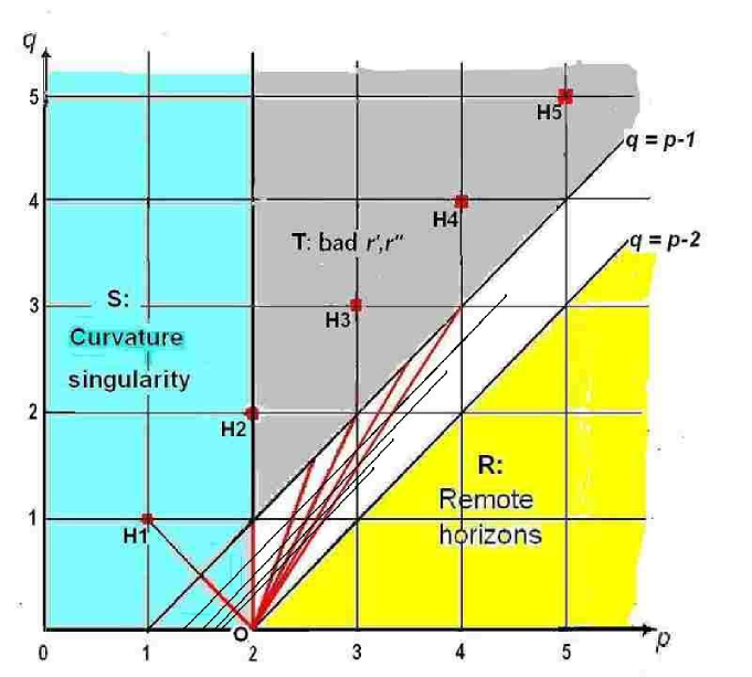
Figure 1: Properties of the candidate horizon $r=r_{h}$ depending on $p$ and $q$. Horizons admitting extensions correspond to the points H1, H2,… ($p=q\in{\mathbb{N}}$) and other points (32), some of which (with $k=2,\ldots,6$) are shown by intersections of the beams (30) originating at point O with the line $q=p-1$ and with the thin lines parallel to it. Under the weakened condition on $r(u)$, namely, that $r^{\prime}$ and $r^{\prime\prime}$ should be finite, admissible are whole segments of the beams (30), belonging to the band (34). In region S ($p<2$), outside the segment OH1, $r=r_{h}$ is a curvature singularity. Outside the other beams (30), an extension of the metric beyond the sphere $r=r_{h}$ is impeded by fractional powers in $A(u)$ and, in region T, by infinities in $r^{\prime}$ (in case $q>p$) and $r^{\prime\prime}$. In region R, including the line $q=p-2$, $r=r_{h}$ is a remote horizon.

 

Now we are ready to compare the above results with the classification of horizons ZP ; Z as “usual”, “naked” and “truly naked” in terms of the metric (25) under the assumption (27). A criterion for distinguishing them is Z

$$\begin{array}[]{ll}{\rm usual:}&{\widetilde{Z}}(r_{h})=0,\\ {\rm naked:}&{\widetilde{Z}}(r_{h})\ {\rm finite},\\ {\rm truly\ naked:}&{\widetilde{Z}}(r_{h})=\infty,\end{array}$$ (35)

where the quantity ${\widetilde{Z}}$, characterizing the magnitude of tidal forces at $r=r_{h}$ in a freely falling reference frame, is given by [see (5)]

$${\widetilde{Z}}={\rm const}\cdot(q-p)(r-r_{h})^{p-1-q}.$$ (36)

Its counterpart in the static reference frame is $Z={\rm const}\cdot(q-p)(r-r_{h})^{p-1}$, which is zero at all candidate horizons.

We would like to stress that only transversal components of the curvature tensor are relevant to our discussion. The reason is that the $R^{tr}{}_{tr}$ component of the Riemann tensor, which characterizes tidal forces in the radial direction, does not change under radial boosts. So if it is finite, it is irrelevant to the issue of singularities while if it diverges, we evidently deal with a curvature singularity for which the Kretschamnn scalar diverges.

The results of such a comparison are collected in Table I. The table mentions one more quantity, $Q$, that distinguishes usual and naked horizons in the case $p=q$ Z ,

$$Q=2(\alpha_{r}+\gamma_{r}),$$ (37)

which depends on further details of the behavior of $\alpha$ and $\gamma$ as compared with (27).

Table 1: Horizon types according to Refs. ZP ; Z and the results of the present analysis. Curvature ($C^{0}$) singularities are not included.

No.	$p,\ q$	type by (35)	present analysis
1	$p=q=1$	usual or naked∗	regular, $n=1$
2	$1<p<{\textstyle\frac{3}{2}}$, $q=2-p$	truly naked	singular
3	$p={\textstyle\frac{3}{2}},\ q={\textstyle\frac{1}{2}}$	naked	regular, $n=1$
4	${\textstyle\frac{3}{2}}<p<2$, $q=2-p$	usual	regular, $n=1$
5	$p\geq 2,\ q>p$	truly naked	singular
6	$p\geq 2,\ q=p$	usual or naked∗	regular if $p=q=n$, otherwise singular
7	$p\geq 2,\ p-1<q<p$	truly naked	singular
8	$p\geq 2,\ q=p-1$	naked	regular if $p=1+n/2$, otherwise singular
9	$p\geq 2,\ p-2<q<p-1$	usual	regular if (30) holds, $n\in{\mathbb{N}}$, otherwise singular
10	$p\geq 2,\ q\leq p-2$	usual	remote horizon

^∗ The horizon is usual if $Q=0$ and naked if $Q\neq 0$ at $r=r_{h}$ with $Q$ defined in Eq. (37).

In the fourth column, the word ‘regular’ means that the above criteria (a), (b) are fulfilled, $r^{\prime}$ and $r^{\prime\prime}$ are finite, and an (at least $C^{2}$) extension is possible; though, on the segments (30) (34) (lines 4, 9 of the table), this extension can be analytic only at the countable number of points (32). The term ‘singular’ means impossibility of an extension, though all algebraic curvature invariants are finite.

From the viewpoint of a general classification of space-time singularities (see, e.g., e-sch77 ), what we usually call a curvature singularity [a set of (limiting) space-time points with an infinite value (or discontinuity) of at least one algebraic invariant of the Riemann tensor] is called a $C^{0}$ curvature singularity. A more general notion is that of a $C^{m}$ curvature singularities, related to a discontinuity in some of the tetrad components of the $m$-th covariant derivatives of the Riemann tensor. (In many cases, but not always, at such singularities, some invariants involving derivatives of the Riemann tensor are discontinuous.) The singularities discussed here are apparently related to such higher-order curvature singularities, but this relation is quite nontrivial, and its exact formulation requires a separate study which is beyond the scope of this paper.

Table I shows that all TNHs and (somewhat unexpectedly) many of the “simply” naked horizons and even some “usual” ones are actually space-time singularities in the sense that geodesics terminate there at finite values of the canonical parameter.

One can remark that analytic properties of the metric near a horizon are often discussed in terms of the two-dimensional ($t,R$) submanifold, assuming the angular part of the metric to be irrelevant. We have seen that, on the contrary, it is the behavior of the derivatives $r^{\prime}$ and $r^{\prime\prime}$ that makes singular many candidate horizons looking quite regular in the ($t,R$) submanifold.

V Examples

V.1 Naked and “potentially naked” horizons

At event horizons of naked black holes according to Z ; ZP , the quantity ${\widetilde{Z}}$ [see (5) or (36)] is finite. To be naked according to HR1 ; HR2 , such a horizon must exhibit large values of ${\widetilde{Z}}$ on the Planck scale while the curvature invariants remain small on the same scale. Let us discuss the relationship of these notions using as an example the dilaton black hole solution bsh77 ; GM ; GHS92 , discussed in HR1 , with the metric (2) such that

$$A=\frac{(u-u_{+})(u-u_{-})}{r^{2}},\hskip 28.45274ptr=u\biggl{(}1-\frac{u_{-}}{u}\biggr{)}^{b},\hskip 28.45274pt0<b<1,$$ (38)

with $b={\rm const}$. There is a horizon at $u=u_{+}>u_{-}$ and a singularity at $u=u_{-}$. The extremal limit corresponds to $u_{+}=u_{-}$, and in this limit the horizon area shrinks, $r_{+}=r(u_{+})\to 0$, leading to a singularity.

Then, simple calculations give

$$Z=-\frac{r^{\prime\prime}}{r}A,\hskip 28.45274pt{\widetilde{Z}}\sim\frac{Z}{A}=-\frac{r^{\prime\prime}}{r}=-\frac{u_{-}b(b-1)}{u^{3}}\biggl{(}1-\frac{u_{-}}{u}\biggr{)}^{-2}.$$ (39)

We see that ${\widetilde{Z}}(u_{+})$ is finite, so that the horizon is naked according to Z ; ZP .

The curvature components in the static frame are of the order $1/r_{+}^{2}$. Introducing the parameter $\varepsilon=1-r_{-}/r_{+}$, we obtain that near the horizon ${\widetilde{Z}}\sim u_{+}^{-2}\varepsilon^{-2}$ and $r_{+}^{-2}\sim u_{+}^{-2}\varepsilon^{-b}$. In the limit $\varepsilon\to 0$, both ${\widetilde{Z}}$ and the curvature invariants become infinite as $u\to u_{+}=u_{-}$ since $u=u_{-}$ is a singularity. If, however, one chooses an intermediate value of $\varepsilon$ such that

$$\left(\frac{l_{Pl}}{u_{+}}\right)^{2/b}\ll\varepsilon\ll 1,$$ (40)

so that $u_{+}\gg l_{Pl}$, where $l_{Pl}$ is the Planck length, we arrive at the situation that the tidal forces are large but the curvature components in the static frame (and hence the curvature invariants) remain small on the Planck scale HR1 .

Thus the naked behavior of this black hole is due to proximity to the singularity. As to the general case (38), (39), its naked nature according to (35) ZP ; Z only indicates that this solution can really exhibit a naked behavior at some values of its parameters. In this sense, as was said in the Introduction, such horizons (and black holes) may be called “potentially naked” as opposed to naked ones according to Horowitz and Ross and truly naked ones which are always singular as follows from our present results.

V.2 Matter with an arbitrary equation of state

Consider again the metric (2) and the Einstein equations for it with the stress-energy tensor $T_{\mu}^{\nu}=T_{\mu}^{\nu}{}_{(m)}+T_{\mu}^{\nu}{}_{\rm(vac)}$ where

$$T_{\mu(m)}^{\nu}=\mathop{\rm diag}\nolimits(\rho,\ -p_{r},-p_{\bot},\ -p_{\bot}).$$ (41)

is the contribution of some kind of matter (e.g., a perfect fluid) and

$$T_{\mu}^{\nu}{}_{\rm(vac)}=\mathop{\rm diag}\nolimits(\rho{}_{\rm(vac)},\ \rho{}_{\rm(vac)},\ -p_{\bot}{}_{\rm(vac)},\ -p_{\bot}{}_{\rm(vac)}).$$ (42)

is that of a so-called vacuum fluid, distinguished by the property $T_{0}^{0}=T_{1}^{1}$ dym . Particular cases of such “vacua” are a cosmological constant ($p_{\bot}{}_{\rm(vac)}=-\rho{}_{\rm(vac)}=-\Lambda/(8\pi)$), electric or magnetic fields in the radial direction ($p_{\bot}{}_{\rm(vac)}=\rho{}_{\rm(vac)}$) and other forms which may be specified, e.g., by $\rho{}_{\rm(vac)}$ as a function of $r$ dym ; br-NED ; eliz1 ; eliz2 .

Let us choose, as independent components of the Einstein equations, the difference ${0\choose 0}-{1\choose 1}$ and the ${1\choose 1}$ equation which read

$$2A\frac{r^{\prime\prime}}{r} = -8\pi(\rho+p_{r}),$$ (43)

$$\frac{1}{r^{2}}(-1+A^{\prime}rr^{\prime}+Ar^{\prime}{}^{2}) = 8\pi(p_{r}-\rho{}_{\rm(vac)}).$$ (44)

In addition, assuming no interaction between matter and vacuum, we can write the conservation law for matter in the form

$$p^{\prime}_{r}+\frac{2r^{\prime}}{r}(p_{r}-p_{\bot})+\frac{A^{\prime}}{2A}(\rho+p_{r})=0.$$ (45)

and similarly for vacuum.

Let us also assume that the matter obeys the linear equation of state (at least approximately, near the horizon)

$$p_{r}\approx w\rho,\ \ \ w={\rm const}.$$ (46)

Then, a further analysis can be carried out along the lines of bz2 , with the only difference that now we do not restrict ourselves to only regular horizons and seek any solutions with $A\to 0$ as $u\to u_{h}$ where $u_{h}\neq\infty$. In particular, we do not require that $r^{\prime}$ and $r^{\prime\prime}$ should be finite as $u\to u_{h}$. Omitting the details, we present the results.

We obtain that if there is no vacuum ($T_{\mu}^{\nu}{}_{\rm(vac)}=0$), then the only possible solutions correspond to a simple horizon, such that $A(u)\sim u-u_{h}$, and, provided $w=-1/(1+2k)$ where $k$ is a positive integer, we obtain regular solutions in full agreement with bz2 . Solutions with TNHs are not obtained. The value $w=-1$ is excluded since it corresponds to a vacuum fluid, contrary to what was assumed.

If, however, we consider a mixture of the two kinds of matter described by (41) and (42), there appear solutions containing matter with $0>w>-1$ and $\rho\sim A^{-(w+1)/(2w)}$. Furthermore, if we turn to the curvature coordinates and assume that the metric coefficients behave according to (27), we obtain, for $p\neq q$, the following relation:

$$w=-q/(q+2p-2),$$ (47)

and it appears that $\rho>0$ for $q>p$ and $\rho<0$ for $q<p$. Thus any $p$ and $q$ satisfying the condition (28) are admissible, except for those with $p=q$. In the latter case, solutions can also exist, with $w$ satisfying the requirement $w>-p/(3p-2)$.

All kinds of solutions mentioned in Table I are possible, and the values of $w$ cover the whole range from 0 to $-1$. This is related to the underdetermined nature of the system since the function $\rho{}_{\rm(vac)}(u)$ remains arbitrary.

If we put $\rho{}_{\rm(vac)}=\Lambda/(8\pi)={\rm const}$, thus specifying the vacuum as a cosmological constant, the Einstein equations relate the exponents $p$ and $q$ characterizing the metric to the matter parameter $w$. Namely, we have either (i) $p=q=1$ (a simple regular horizon) and $w=-1/(1+2k)$ (as described in bz2 ) or (ii)

$$p=2,\hskip 28.45274ptq=-2w/(w+1),\hskip 28.45274ptw\neq-1/2.$$ (48)

The parameter $w$ can take any value in the range $(-1,\ 0)$ except $-1/2$. The configurations correspond to lines 5, 7, 8, 9 of Table I.

V.3 Scalar field with a potential

Consider a real, minimally coupled scalar field $\phi$ with the Lagrangian $L_{s}=(16\pi)^{-1}[\epsilon g^{\mu\nu}\partial_{\mu}\phi\partial_{\nu}\phi-2V(\phi)]$ as a source of gravity. Here, $V(\phi)$ is a potential while $\epsilon=1$ corresponds to normal fields with a correct sign of the kinetic energy and $\epsilon=-1$ to the so-called phantom fields, often discussed in the context of the dark energy problem.

Then static, spherically symmetric configurations with the metric (2) and $\phi=\phi(u)$ obey the equations

$$(Ar^{2}\phi^{\prime})^{\prime} = \varepsilon r^{2}dV/d\phi,$$ (49)

$$(A^{\prime}r^{2})^{\prime} = -2r^{2}V,$$ (50)

$$2r^{\prime\prime}/r = -\varepsilon{\phi^{\prime}}^{2},$$ (51)

$$A(r^{2})^{\prime\prime}-r^{2}A^{\prime\prime} = 2.$$ (52)

Eq. (49) follows from (50)–(52), which, given a potential $V(\phi)$, form a determined set of equations for the unknowns $r(u),\ A(u),\ \phi(u)$. Eq. (52) is once integrated giving

$$\biggl{(}\frac{A}{r^{2}}\biggr{)}^{\prime}=\frac{2(u_{0}-u)}{r^{4}},$$ (53)

where $u_{0}$ is an integration constant.

Let us assume that $u=0$ is a candidate horizon, near which

$$A\approx A_{n}u^{n}(1+o(1)),\hskip 28.45274ptr=r_{h}+r_{k}u^{k}+o(u^{k}),$$ (54)

where $n>0,\ A_{n}>0,\ r_{h}>0,\ r_{k}$ are constants. According to Sec. IV, at a regular horizon, $n$ and $k$ should be positive integers. In particular, $|r^{\prime\prime}|<\infty$, and Eq. (51) yields a finite value of $\phi^{\prime}$. As a result, one can arrive at different black hole solutions with particular potentials (see, e.g., mann ; vac1 ; vac2 and references therein), including globally regular solutions for phantom fields (the so-called black universes bu12 ).

Our interest here is, however, in the existence of solutions containing TNHs, let us therefore assume $k\not\in{\mathbb{N}}$. Then Eq. (51) in the leading order of magnitude gives

$$\phi^{\prime}\approx\pm\phi_{1}u^{k/2-1},\hskip 28.45274pt\phi_{1}:=\sqrt{-2\epsilon k(k-1)r_{k}/r_{h}},$$ (55)

so that, evidently, we must have $(k-1)\epsilon r_{k}<0$. Choosing the upper sign and integrating, we have

$$\phi\approx\phi_{0}+\frac{2\phi_{1}}{k}u^{k/2},\hskip 28.45274pt\phi_{0}={\rm const}.$$ (56)

On the other hand, Eq. (53) in the leading order of magnitude gives different results for $u_{0}=0$ and $u_{0}\neq 0$, namely,

$${}n=1,\hskip 28.45274ptA_{1}r_{h}^{2}=2u_{0}\hskip 28.45274pt{\rm for}\ \ u_{0}\neq 0,$$

$${}n=2,\hskip 28.45274ptA_{2}r_{h}^{2}=-1\ \ \hskip 28.45274pt{\rm for}\ \ u_{0}=0.$$ (57)

The second case is excluded due to the requirement $A_{2}>0$. So we are left with the first line in (V.3), and the main point is that $A(u)$ is automatically well-behaved and corresponds to a simple horizon ($n=1$) irrespective of the value of $k$.

Substituting the expressions for $r$ and $A$ into Eq. (50), we find that $V$ tends to infinity as $u\to 0$ (thus leading to a curvature singularity) if $k<1$ and to a finite limit if $k>1$. Thus we must have $k>1$ in Eq. (54).

An asymptotic form of $V(\phi)$ as $\phi\to\phi_{0}$ is easily obtained using Eq. (49) which yields $dV/d\phi$. As a result, we have

$$V(\phi)\approx V_{0}+{\rm const}\cdot(\phi-\phi_{0})^{2(k-1)/k}.$$ (58)

Thus there exist solutions in the form of singular horizons for potentials having the asymptotic form (58), i.e., at values $\phi=\phi_{0}$, if any, approached with fractional powers of $\phi-\phi_{0}$ (recall that we have been considering $k\not\in{\mathbb{N}}$).

Passing over to the curvature coordinates using (26), we see that the above asymptotic solution is described by the conditions (27) where $p$ and $q$ are expressed in terms of $k$ according to (32) with $n=1$, i.e., $p=2-1/k$, $q=1/k$. In other words, these solutions reside on the segment OH1 in Fig. 1 and correspond to lines 2,3,4 in Table I.

V.4 $(2+1)$-dimensional analogue: an exact solution

We have given examples of TNHs in some solutions of general relativity by analyzing the near-horizon geometry. Unlike that, in $(2+1)$-dimensional general relativity it is possible to present an exact solution with a horizon, where the source of gravity is a perfect fluid with a linear equation of state, such that

$$T_{\mu}^{\nu}=\mathop{\rm diag}\nolimits(\rho,\ -p,\ -p),\hskip 28.45274ptp=w\rho,\ \ w={\rm const}.$$ (59)

This solution can be extracted from the results of Ref. ext , a study aimed at finding all possible static analogues of the Bertotti-Robinson space-time without requiring spherical symmetry. A $(2+1)$-dimensional section of one of the classes of space-times obtained there has a circularly symmetric metric similar to 4D spherically symmetric metrics with a TNH. The metric has the form

$$ds^{2}={\,\rm e}^{2\gamma}dt^{2}-{\,\rm e}^{2\alpha}dr^{2}-r^{2}d\phi^{2},$$ (60)

where

$${\,\rm e}^{2\alpha}=\left(\frac{r_{0}^{2}-r^{2}}{r_{0}^{2}}\right)^{-2/(1-w)},\hskip 28.45274pt{\,\rm e}^{2\gamma}={\rm const}\cdot(r_{0}^{2}-r^{2})^{-2w/(1-w)},$$ (61)

and the density is

$$\rho=\frac{(r_{0}^{2}-r^{2})^{\eta}}{4\pi(1-w)r_{0}^{4/(1-w)}},\hskip 28.45274pt\eta=\frac{1+w}{1-w}.$$ (62)

A candidate horizon, at which ${\,\rm e}^{\gamma}=0$, is $r=r_{0}$ if $w<0$ or $w>1$. In its neighborhood,

$${\widetilde{Z}}\sim{\,\rm e}^{-2\gamma}Z\sim{\,\rm e}^{-2\gamma}\rho\sim(r_{0}^{2}-r^{2})^{\varepsilon},\hskip 28.45274pt\varepsilon=\frac{1+3w}{1-w}.$$ (63)

Eq. (63) does not work for $w=-1$ corresponding to a cosmological constant and 3D de Sitter metric, in which case $Z={\widetilde{Z}}=0$.

The density is finite or zero at $r=r_{0}$ if $\eta\geq 0$, and it can be verified that the Kretschmann scalar is finite under the same condition. Thus a curvature singularity at $r=r_{0}$ is absent in the whole range $-1\leq w<1$, but possible horizons for $w>1$ are excluded. On the other hand, if $\varepsilon<0$, then ${\widetilde{Z}}$ diverges, so that the tidal forces in the freely falling frame are infinite, and for

$$-1<w<-1/3$$ (64)

we have a solution with a TNH. Recall for comparison that in 4 dimensions (Sec. V.B) TNHs appeared in solutions with a similar source in the range $-1<w<0$ and only in the presence of a vacuum fluid.

Table 2: Horizon types in the solution (60)–(62) in the range $-1\leq w<1$.

No.	$w$	horizon type by (35)	present analysis
1	$w\in(0,\,1)$	no horizon
2	$w\in(-1/3,\,0)$	usual	regular if (65) holds, otherwise singular
3	$w=-1/3$	naked	regular, $n=1,\ k=2$
4	$w\in(-1,\,-1/3)$	truly naked	singular
5	$w=-1$	usual	regular, $n=1,\ k=1$

An analysis similar to that of Sec. IV leads to the results presented in Table II. The terminology is the same as in Table I: e.g., the word “regular” means that the metric can be extended beyond the horizon. It is of interest that a transition to the quasiglobal coordinate $u$ similar to (26) leads, for any $w<0$, to $A\sim u$, i.e., to a first-order horizon ($n=1$), which is, however, not always regular due to the behavior of $r(u)$. To satisfy the regularity criterion (c) [see Eq. (21)], the parameter $w$ should be related to $k\in{\mathbb{N}}$ by

$$w=-1/(2k-1).$$ (65)

As in 4 dimensions, all TNHs turn out to be singular, and even those horizons that seem usual can be singular as well (see line 2 of Table II).

VI Horizons in Kantowski-Sachs cosmologies

VI.1 Regular horizons

It is easy to reformulate the regular horizon conditions like (23) and (24) for a time-dependent homogeneous analogue of static, spherically symmetric space-times, i.e., KS cosmologies.

A KS metric written in terms of an arbitrary time coordinate $t$ reads

$$ds^{2}=b^{2}(t)dt^{2}-a^{2}(t)dx^{2}-r^{2}(t)d\Omega^{2}.$$ (66)

with an arbitrary lapse function $b(t)$ and two scale factors $a(t)$ and $r(t)$. Identifying the metrics (6) and (66) and applying the requirements (a), (b), (c) from Sec. IV to (6) precisely as in static spherical symmetry, we arrive at the following necessary conditions of a regular (extensible) horizon at a value of $t$ at which $a\to 0$:

$${}\frac{1}{b}\frac{da}{dt}\sim u^{n-1}\sim a^{2(n-1)/n},$$ (67)

$${}\frac{1}{b}\frac{dr}{dt}\sim u^{n/2+k-1}\sim a^{(n+2k-2)/n}$$ (68)

Here, as before, $n\in{\mathbb{N}}$ is the order of the horizon and $k\in{\mathbb{N}}$ corresponds to Eq. (21).

One can also modify the results of Sec. IV for a cosmological analogue of the curvature coordinate, i.e., the scale factor $r(u)$ considered as a coordinate. It seems, however, more helpful to present detailed horizon regularity conditions for the metric (7) written in terms of the proper time $t=\tau$, most widely used in cosmology as a natural time variable. Identifying (6) and (7) term by term, we have

$$d\tau=\pm\frac{du}{\sqrt{A(u)}},\hskip 28.45274pta^{2}(\tau)=A(u),\hskip 28.45274ptr(\tau)=r(u).$$ (69)

Applying again the requirements (a), (b), (c) from Sec. IV, we obtain the following properties of the metric (7) at a regular horizon occurring at a value of $\tau$ where $a\to 0$ and $r\to r_{h}>0$.

1. A horizon may correspond to finite or infinite $\tau$. In the latter case, the integral $u=\int a(\tau)d\tau$ should still converge, otherwise we deal with a remote horizon in the absolute past or future, attained by all geodesics at infinite values of their canonical parameters.

2. A first-order horizon ($n=1$) occurs at finite $\tau=\tau_{h}$, near which

$$a(\tau)\sim\tau-\tau_{h},\hskip 28.45274ptr(\tau)\approx r_{h}+C(\tau-\tau_{h})^{2k},$$ (70)

where $r_{h}$ and $C$ are constants and $k\in{\mathbb{N}}$ is the exponent from the condition (21).

3. A second-order horizon ($n=2$) is characterized by

$$\tau\to\pm\infty,\hskip 28.45274pta(\tau)\sim{\,\rm e}^{-m|\tau|},\hskip 28.45274ptr(\tau)\approx r_{h}+C{\,\rm e}^{-km|\tau|}$$ (71)

with $m={\rm const}>0$.

4. At higher-order horizons ($n\geq 3$), we have

$$\tau\to\pm\infty,\hskip 28.45274pta(\tau)\sim|\tau|^{-n/(n-2)},\hskip 28.45274ptr(\tau)\approx r_{h}+C|\tau|^{-2k/(n-2)}.$$ (72)

Thus horizons of any order $n$ are possible in the past (or future) of a KS universe. As argued in bd07 ; bz1 , a matter source for such a behavior of the metric is probably pure vacuum since, among other kinds of matter, only that with some particular values of $w\leq-3$, which may be called “deeply phantom”, is admissible bz1 . It has been concluded bd07 ; bz1 that normal matter could have been created later from vacuum along with isotropization.

We also see that regular horizons of orders 2 and higher occur at infinite proper times of observers at rest in KS space-times. In other words, if the present cosmological evolution began at such a horizon, it has happened infinitely long ago. However, other geodesic paths, both timelike and null, cross such horizons at finite values of their canonical parameters (due to finite quasiglobal time $u$), and one can conclude that one-way communication with regions beyond such horizons is still possible (this phenomenon was discussed in detail for vacuum KS cosmologies in bdd03 ). If we live in such a universe, we can in principle catch photons or massive particles coming from an infinitely remote past according to our own clocks.

This situation is fundamentally different from that of a remote horizon in the past, where $u\to-\infty$, which is also possible but bz1 only in the presence of matter with $w\leq-3$.

VI.2 General analysis

All behaviors of $a(\tau)\to 0$ and $r(\tau)$ other than those enumerated in items 1-4 of the previous subsection either correspond to singular horizons (in the sense explained above) or to curvature singularities. A curvature singularity is avoided if [see (II), the dot denotes $d/d\tau$]

$$|{\ddot{a}}/a|,\quad\ |{\dot{a}}{\dot{r}}/a|,\quad\ |\ddot{r}|\ \ \ {\rm are\ finite.}$$ (73)

It is still of interest to analyze tidal forces acting on different geodesic observers in more general metrics with $a\to 0$, satisfying (73), and to compare the results with the above horizon regularity conditions.

Let us separately consider horizons with different asymptotics, generalizing the expressions (70)–(72).

First, assuming a horizon at finite $\tau=\tau_{h}$ and $a(\tau)\sim(\tau-\tau_{h})^{m}$, the condition $|\ddot{a}/a|<\infty$ immediately leads to $m=1$, hence $A(u)\sim u$, it is a first-order horizon ($n=1$). We can put

$$a(\tau)\sim\tau-\tau_{h},\hskip 28.45274ptr(\tau)\approx r_{h}+C(\tau-\tau_{h})^{s},$$ (74)

with some constants $C$ and $s$ where $s\geq 2$ by virtue of (73). Regular horizons, as we know from (70), correspond to $s=2k$, $k\in{\mathbb{N}}$.

Second, for infinite $\tau$ at the horizon, we can take by analogy with (71)

$$\tau\to\pm\infty,\hskip 28.45274pta(\tau)\sim{\,\rm e}^{-m|\tau|},\hskip 28.45274ptr(\tau)\approx r_{h}+C{\,\rm e}^{-s|\tau|},\hskip 28.45274ptm>0,\ \ s>0.$$ (75)

with arbitrary constants $m$ and $s$. Regular horizons correspond to $s=km$, $k\in{\mathbb{N}}$.

Third, in a similar way, we can take by analogy with (72)

$$\tau\to\pm\infty,\hskip 28.45274pta(\tau)\sim|\tau|^{-m},\hskip 28.45274ptr(\tau)\approx r_{h}+C|\tau|^{-s},\hskip 28.45274ptm>0,\ \ s>0.$$ (76)

Regular horizons correspond to

$$m=\frac{n}{n-2},\hskip 28.45274pts=\frac{2k}{n-2},\hskip 28.45274ptn=3,4,\ldots,\ \ k\in{\mathbb{N}}.$$ (77)

Performing an analysis similar to that of Sec. IV, we arrive at Table 3.

Table 3: Types of horizons in KS cosmology

No.	$a,\ r$	$m,\ s$	type by (35)	type by extensibility	$w$
1	(74)	$s=2$	usual or naked	regular, $n=1$	$w=-3$
2	(74)	$2<s<4$	truly naked	singular	$-3<w<-1$
3	(74)	$s\geq 4$	usual or naked	regular, $n=1$, only if $2s=k\in{\mathbb{N}}$	$w\leq-3$
4	(75)	$m>0,\ s=m$	usual or naked	regular, $n=2$	$w=-3$
5	(75)	$m>0,\ m<s<2m$	truly naked	singular	$-3<w<-2$
6	(75)	$m>0,\ s\geq 2m$	usual or naked	regular, $n=2$, only if $s/m=k\in{\mathbb{N}}$	$w\leq-3$
7	(76)	$m>1,\ s<2(m-1)$	truly naked	singular	$-3<w<-{\textstyle\frac{5}{3}}$
8	(76)	$m>1,\ s=2(m-1)$	naked	regular, $n\geq 3$, only if (77) holds	$w=-3$
9	(76)	$m>1,\ s>2(m-1)$	usual	regular, $n\geq 3$, only if (77) holds	$w<-3$

As before, the presence of a TNH means that an observer moving along a timelike geodesic and reaching the horizon experiences infinite tidal forces. However, for a comoving observer, similar to a static observer in space-times considered above, the tidal forces [as well as all the curvature components (II)] are finite. The cosmological scenarios thus look differently for different groups of observers. Consider, for example. a TNH corresponding to line 2 of Table III. Then, an observer at rest reaches it at finite proper time and would be able to cross it if it were possible. However, an observer which follows a timelike geodesics with non-zero velocity with respect to the environment is subject to infinitely growing tidal forces and will be destroyed before reaching the horizon. This also applies to higher-order TNHs (lines 5 and 7 of Table III). In the latter case, however, an observer at rest, for whom the tidal forces would be finite, never reaches the horizon since it would require an infinite time.

It is also of interest to elucidate which kinds of matter are compatible with the space-times under discussion. Considering a non-interacting mixture of a vacuum fluid and an arbitrary kind of matter with the parameter $w=p_{x}/\rho\neq-1$ ($p_{x}=-T^{x}_{x}$ is the pressure in the $x$ direction; $w=-1$ corresponds to the vacuum fluid) in the manner of Sec. V.B and Ref. bz1 , we obtain the last column of Table III with appropriate values of $w$. All of them correspond to phantom matter.

If there is no vacuum fluid, only simple regular horizons described by line 1 are possible, in agreement with the results of Sec. V.B and Ref. bz1 .

A comparison shows that, for cosmological metrics, the parameter $w$ behaves like $1/w$ for static metrics. This is not surprising since, in a sense, the energy density and the radial pressure interchange their roles when we change $A\to-A$. Curiously, according to Table III, cosmological metrics with TNHs require less exotic matter than those with a regular horizon.

It is worth noting that the so-called nonscalar singularities (to which class the TNHs belong) in cosmology were also discussed in Sec. 4.3 of e-sch77 and in ek ; col , where “tilted cosmologies” with perfect fluids were considered. The latter means that matter flows non-orthogonally to the homogeneity surfaces. A detailed comparison of our results with these papers is beyond the scope of this paper and deserves a separate treatment. Here, we only note that we do not restrict the matter to be necessarily a perfect fluid, and no “tilting” is assumed. In addition, we deal with KS spherically symmetric cosmologies whereas Ref. col considered locally rotationally symmetric Bianchi-V models.

VII Concluding remarks

1. We have obtained the necessary conditions (23), (24) of a regular horizon, admitting a Kruskal-like extension, in terms of the general metric (1), and similar conditions (67), (68) for its cosmological counterpart, the general KS metric (66). Comparing these general regularity conditions with the relations characterizing naked and truly naked horizons, we found that all TNHs and many horizons which seemed to be usual or simply naked represent singularities in the sense that geodesics terminate there at finite values of the canonical parameter.

Our consideration was almost everywhere restricted to neighborhoods of (candidate) horizons, therefore we mostly spoke of naked, etc., horizons rather than black holes. The results are equally applicable to any event, Cauchy or cosmological horizons in static or homogeneous spherically symmetric space-times in the framework of any metric theory of gravity. Moreover, the results obtained can be easily generalized to other space-time symmetries and dimensions.

2. In Sec. V.B, discussing matter with an arbitrary equation of state, we actually obtained that all kinds of horizons mentioned in Table I are possible but only in the presence of some “vacuum fluid” which may be represented by a cosmological constant or an electric or magnetic field. Meanwhile, to be compatible with any kind of horizon (including singular ones), the fluid itself must have negative radial pressure. This generalizes our previous result bz2 that only special kinds of fluids with particular values of the parameter $w=p_{r}/\rho$, including that with $w=-1/3$ (a fluid of disordered cosmic strings), are compatible with regular horizons.

The examples considered show that naked and truly naked horizons do really appear in static solutions to the Einstein equations for certain kinds of matter, not to mention possible solutions of alternative theories of gravity. In particular, they may correspond to equations of state with $w<-1/3$ [see, e.g., (48)] often discussed in the context of non-phantom dark energy, or quintessence.

In the cosmological context, the only kinds of matter compatible with horizons (both regular and singular) are vacuum fluids and phantom matter with $w=p_{x}/\rho<-1$, and a distinguished value compatible with regular horizons is $w=-3$. As in the static case, most of horizon types are only possible in the presence of a vacuum fluid.

3. In considering TNHs, we implicitly assumed that an extended body (or an observer) approaching a horizon and facing infinite tidal forces moves along a geodesic. Meanwhile, it is reasonable to ask what can happen in a more general situation. Is it possible to adjust the motion of an accelerated body in such a way that, even at a TNH, it could be subject to finite tidal forces unlike a geodesic observer?

A direct inspection shows that it is really possible to avoid infinite tidal forces at a TNH by properly choosing a non-geodesic path. However, an inevitable price for this is that the acceleration experienced by such an observer tends to infinity when approaching the horizon. The calculations are carried out separately for the cases when the proper distance to the horizon is finite or infinite (the details will be presented elsewhere). The resulting infinite acceleration can be viewed as one more manifestation of a really singular nature of TNHs.

An important point is, however, that a singular nature of many horizons in the sense of extensibility is not directly related to their “truly naked” character: we have seen that many horizons which do not create large or infinite tidal forces, are still inextensible. A reason for that evidently consists in the properties of matter in the near-horizon region, incompatible with analyticity of the functions $A(u)$ and $r(u)$.

4. A phenomenon of interest in KS cosmologies is the opportunity to receive information in the form of massive or massless particles from an epoch beyond a past horizon (if any), even though such a horizon could occur infinitely long ago according to our clocks. In reality, all such particles would be probably absorbed at a subsequent hot stage of the Universe evolution; but the existence of their traces in observable phenomena, e.g., in CMB properties, should not be excluded.

5. In the context of the early Universe, in addition to particle creation, it would be of interest to take into account one more quantum phenomenon, the dynamical Casimir effect related to the nontrivial topology of KS models, e.g., in the manner of Refs. NO99 , and its possible influence on the structure of singularities like those discussed in this paper.

It would also be of interest to relate the origin of singularities in KS cosmology subject to quantum effects with their effective 2D description, in the manner of nooo99 , where quantum-corrected KS cosmologies were investigated. The effective 2D description makes the presentation qualitatively easier and may reveal a fundamental structure behind singularities, related to quantum effects.

6. The singular horizons in KS cosmology discussed in this paper (at least simple ones) may be considered as examples of the so-called finite-time singularities. Four types of such singularities are known and classified for isotropic FRW models in Ref. NOTs05 . Among them, the Big Rip (or type I singularity) is the most well-known and is widely discussed in connection with different models of dark energy. It is clear that in KS models, where we have two scale factors, such singularities may occur and their properties should be more diverse, and the corresponding classification should be naturally extended as compared with the one-scale-factor FRW cosmology. Such an extended classification, which should also apply to static, spherically symmetric analogues of KS cosmologies as well as to other, more complicated anisotropic cosmologies, is of significant interest. Let us mention some tentative results on this way.

The Big Rip singularity in FRW models consists in an infinite growth of the scale factor $a(\tau)$ at finite proper time $\tau$, accompanied by $\rho\to\infty$, where $\rho$ is the density of matter with $w<-1$. Considering such a fluid, with $w=p_{x}/\rho=p_{\bot}/\rho<-1$ in the KS geometry (7), we obtain that a Big Rip can also occur at finite $\tau=\tau_{s}$ but can be both isotropic and anisotropic: the volume factor $v$ and the density $\rho$ behave in the same way as in FRW models:

$$v(\tau)=a(\tau)r^{2}(\tau)\sim|\tau-\tau_{s}|^{2/(1+w)},\hskip 28.45274pt\rho(\tau)\sim|\tau-\tau_{s}|^{-2},$$ (78)

but there can be an arbitrary ratio $N$ between the growth rates of $a(\tau)$ and $r(\tau)$, depending on initial conditions: $(\ln a)\dot{}/(\ln r)\dot{}=N={\rm const}>0$. In a similar way, we can discuss singularities of other types, as is done in Ref. NOTs05 .

Static analogues of the Big Rip exist with $w=p_{r}/\rho=p_{\bot}/\rho$ between zero and $-1$, in agreement with the above-mentioned $w\longleftrightarrow 1/w$ correspondence. An opportunity of interest is that $r\to r_{s}>0$ while $A\to\infty$ (a repulsive singularity on a sphere of finite radius) as the coordinate $u$ in (2) tends to a finite value $u_{s}$. The asymptotic behavior is

$$A\sim(u-u_{s})^{-n},\hskip 28.45274ptr\approx r_{s}+r_{k}(u-u_{s})^{k},\hskip 28.45274pt\rho\sim A^{m},$$ (79)

for a fluid with $w=-1/(2m+1)$. Here, the exponents $k>1$, $n>0$ and $m>0$ (but $m\neq 1$) are connected by the relation $n(s-1)=2-k$.

Further details and other results on this subject will be presented elsewhere.

Acknowledgments

K.B. acknowledges partial financial support from Russian Basic Research Foundation Project 07-02-13614-ofi_ts. E.E. and S.D.O. acknowledge support from MEC (Spain), projects FIS2006-02842 and 2005SGR-00790, and S.D.O. from MEC (Spain), project PIE2007-50/023.

References

- (1) G.T. Horowitz and S.F. Ross, Phys. Rev. D 56, 2180 (1997).
- (2) G.T. Horowitz and S.F. Ross, Phys. Rev. D 57, 1098 (1998).
- (3) V. Pravda and O.B. Zaslavskii, Class. Quantum Grav. 22, 5053 (2005).
- (4) O.B. Zaslavskii, Phys. Rev. D 76, 024015 (2007).
- (5) R. Wald, General Relativity (Univ. of Chicago Press, 1984).
- (6) F. J. Tipler, C. J. S. Clarke, and G. F. R. Ellis, in: “General Relativity and Gravitation”, Vol. 2, pp. 97–206, Plenum, New York-London, 1980.
- (7) E. Poisson and W. Israel, Phys. Rev. Lett. 63, 1663 (1989).
- (8) P.R. Brady, in: “Black Holes and Gravitational Waves”, Progr. Theor. Phys. Suppl. No. 136, 29–44 (1999).
- (9) B. C. Nolan, Phys. Rev. D 60, 024014 (1999).
- (10) A. Ori, Phys. Rev. D 61, 064016 (2000).
- (11) P. Aguiar and P. Crawford, Phys. Rev. D 62, 123511 (2000).
- (12) K.A. Bronnikov and I.G. Dymnikova, Class. Quantum Grav. 24, 5803 (2007).
- (13) K.A. Bronnikov and O.B. Zaslavskii, Matter sources for a Null Big Bang, arXiv: 0710.5618; to appear in Class. Quantum Grav. (2008).
- (14) K.A. Bronnikov, Phys. Rev. D 64, 064013 (2001);
- (15) K.A. Bronnikov, G. Clément, C. P. Constantinidis, and J. C. Fabris, Grav. Cosmol. 4, 128 (1998); Phys. Lett. A 243, 121 (1998).
- (16) M. Walker, J. Math. Phys. 11, 2280 (1970).
- (17) K.A. Bronnikov. Inversed black holes and anisotropic collapse. Izv. Vuzov SSSR, Fizika, No. 6, 32 (1979); Russ. Phys. J. 22, 6, 594 (1979).
- (18) T. Klösch and T. Strobl, Class. Quantum Grav. 13, 2395–2422 (1996); 14, 1689–1723 (1997).
- (19) M.O. Katanaev, Nucl. Phys. Proc. Suppl. 88, 233 (2000), gr-qc/9912039; Proc. Steklov Inst. Math. 228, 158–183 (2000), gr-qc/9907088.
- (20) S. Liberati, T. Rothman and S. Sonego, Phys. Rev. D 62, 024005 (2000).
- (21) G.F.R. Ellis and B.G. Schmidt, Gen. Rel. Grav. 8, 915 (1977).
- (22) K.A. Bronnikov and G.N. Shikin, Izv. Vuzov SSSR, Fizika, No. 9, 25 (1977); Russ. Phys. J. 20, 1138 (1977).
-
(23)
G.W. Gibbons, Nucl. Phys. B207, 337 (1982);
G.W. Gibbons and K. Maeda, ibid., B298, 741 (1988). - (24) D. Garfinkle, G.T. Horowitz, and A. Strominger, Phys. Rev. D 43, 3140 (1991); ibid., 45, 3888 (1992).
- (25) K.A. Bronnikov and O.B. Zaslavskii, Phys. Rev. D 78, 021501 (R) (2008). Arxiv: 0801.0889.
- (26) I.G. Dymnikova, Gen. Rel. Grav. 24, 235 (1992); Class. Quantum Grav. 19, 225 (2002); Int. J. Mod. Phys. D 12, 1015 (2003).
- (27) K.A. Bronnikov, Phys. Rev. D 63, 044005 (2001).
- (28) A. Burinskii, E. Elizalde, S.R. Hildebrandt and G. Magli, Phys. Rev. D 65, 064039 (2002).
- (29) E. Elizalde and S.R. Hildebrandt, Phys. Rev. D 65, 124024 (2002).
- (30) K.C.K. Chan, J.H. Horne and R.B. Mann, Nucl. Phys. B 447, 441 (1995).
- (31) K.A. Bronnikov and G.N. Shikin, Grav. Cosmol. 8, 107 (2002).
-
(32)
K.A. Bronnikov and J.C. Fabris, Phys. Rev. Lett. 96, 251101 (2001);
K.A. Bronnikov, V.N. Melnikov and H. Dehnen, Gen. Rel. Grav. 39, 973 (2007). - (33) O.B. Zaslavskii, Class. Quantum Grav. 23, 4083 (2006).
- (34) K.A. Bronnikov, A. Dobosz and I.G. Dymnikova, Class. Quantum Grav. 20, 3797 (2003).
- (35) G.F.R. Ellis and A.R. King, Comm. Math. Phys. 38, 119 (1974).
- (36) C.B. Collins, Comm. Math. Phys. 39, 131 (1974).
- (37) S. Nojiri and S.D. Odintsov, , Int. J. Mod. Phys. A 15, 989 (2000), hep-th 9905089; Phys. Rev. D 59, 044026 (1999), hep-th/9804033.
- (38) S. Nojiri, O. Obregon, S.D. Odintsov and K.E. Osetrin, Phys. Rev. D 60, 024008 (1999); hep-th/9902035.
- (39) S. Nojiri, S.D. Odintsov and S. Tsujikawa, Phys. Rev. D 71, 063004 (2005); hep-th 0501025.