Proper Motion of Milky Way Dwarf Spheroidals from Line-of-Sight Velocities

Abstract

Proper motions for several Milky Way dwarf spheroidal (dSph) galaxies have been determined using both ground and space-based imaging. These measurements require long baselines and repeat observations and typical errors are of order ten milli-arcseconds per century. In this paper, we utilize the effect of “perspective rotation” to show that systematic proper motion of some dSphs can be determined to a similar precision using only stellar line-of-sight velocities. We show that including the effects of small intrinsic rotation in dSphs increases the proper motion errors by about a factor of two. We provide error projections for future data sets, and show that proposed thirty meter class telescopes will measure the proper motion of a few dSphs with milli-arcsecond per century precision.

1. Introduction

The three-dimensional motions of stars and galaxies provide valuable information on the local Universe, ranging from planetary companions of nearby stars to the orbital properties of nearby galaxies and Galactic satellites  (Unwin et al., 2008). However, because measurements of proper motion must be done with respect to cosmic standards of rest, such as background galaxies and quasi-stellar objects, they depend sensitively on the number and nature of background objects in the target field. To obtain measurements of required precision, long baselines and repeat measurements are necessary, ranging from several years for space-based telescopes to tens of years for ground-based telescopes.

Nonetheless, despite their low luminosities, large distances, and small angular separations, about a dozen nearby galaxies now have measured proper motions (Piatek et al., 2007). Among the nearest of these galaxies are the dwarf spheroidals, which have observed luminosities that vary anywhere from a thousand to a million times the luminosity of the Sun. These galaxies are supported primarily by their velocity dispersion and have high mass-to-light ratios $\mathrel{\hbox{\hbox to0.0pt{\hbox{\lower 4.0pt\hbox{$\sim$}}\hss}\hbox{$>$}}}100$ M${}_{\odot}/$ L_⊙  (Mateo, 1998; Łokas et al., 2005; Gilmore et al., 2007; Strigari et al., 2007; Simon & Geha, 2007; Walker et al., 2007). Proper motions have been measured for several Milky Way dSphs (Piatek et al., 2005, 2006, 2007), with errors $\sim 10$ milli-arcseconds per century, corresponding to transverse velocity errors $\sim 100$ km s^-1 for typical dSph distances. In contrast, their velocities in the direction of the observer are now known to $\mathrel{\hbox{\hbox to0.0pt{\hbox{\lower 4.0pt\hbox{$\sim$}}\hss}\hbox{$<$}}}1$ km s^-1.

In this paper, we introduce an alternative technique for determining the proper motions of Milky Way dSphs. Specifically, we utilize present samples of stellar line-of-sight velocities together with the effect known as “perspective rotation,” in which the tangential motion of the galaxy contributes to the measured line-of-sight velocity at large angular separations from the center of the galaxy. Perspective rotation has been detected in Galactic globular clusters (Merritt et al., 1997), and has been used to measure the distance to the Large Magellanic Cloud  (Gould, 2000) and the mass of M31 (van der Marel & Guhathakurta, 2007). Here we show that, using perspective rotation, proper motions of several dSphs can be determined to a precision rivaling the best existing ground and space-based measurements. Additionally, the first proper motion measurements will be possible for several dSphs that are difficult to access via traditional methods.

2. Perspective Rotation

Perspective rotation is simple to understand if we consider the dSphs as extended objects. Because of their close proximity and spatial extent, the line-of-sight velocities of the stars vary as a function of projected radial separation, $R$, from the center of the galaxy. As $R$ increases, the line-of-sight velocities receive increasingly larger contributions from the tangential motion of the object in space. The net result of this radially varying line-of-sight velocity is known as perspective rotation  (Feast et al., 1961). An object that is not rotating intrinsically acquires a velocity gradient that is proportional to the projected distance from the center of the galaxy.

To describe the effect of perspective rotation, we define a cartesian coordinate system in which the $z$-axis points in the direction of the observer from the center of the galaxy, the $x$-axis points in the direction of decreasing right ascension, and the $y$-axis points in the direction of increasing declination. The angle $\phi$ is measured counter-clockwise from the positive $x$-axis, and $\rho$ is the angular separation from the center of the galaxy. The line-of-sight velocity is then

$$v_{los}=v_{x}\sin\rho\cos\phi+v_{y}\sin\rho\sin\phi-v_{z}\cos\rho.$$ (1)

For all of the dSphs that we consider, it is appropriate to use the small angle approximation, $\sin\rho\simeq R/D$, where $R=\sqrt{x^{2}+y^{2}}$, and $D$ is the distance to the dSph. Then using $\sin\phi=y/R$, equation 1 can be written as $v_{los}=v_{x}x/D+v_{y}y/D-v_{z}$. In the limit that $\sin\rho\ll 1$, the line-of-sight velocity is constant across the dSphs and we recover in this limit that $v_{los}=-v_{z}$. It is evident from equation 1 that the transverse velocities $v_{x}$ and $v_{y}$ have the maximal contributions for galaxies that are the appropriate combination of the most nearby and the most spatially extended.

3. Likelihood Function and Error Projections

We define the likelihood function for an observed set of line-of-sight velocities as

$${\cal L}(\vec{\theta})=\prod_{i=1}^{N}\frac{1}{\sqrt{2\pi\sigma_{i}^{2}}}\exp\left[-\frac{1}{2}\frac{(v_{i}-{v_{los}}_{,i})^{2}}{\sigma_{i}^{2}}\right].$$ (2)

Here $\vec{\theta}$ is the set of parameters that describe the model of the galaxy. The product is over the total number of stars, $N$, with measured velocities, and $i$ is an index that represents a star that is located at a fixed projected position. The total velocity dispersion, $\sigma$, is the sum of the intrinsic dispersion, $\sigma_{los}$, and the dispersion from the measurement, $\sigma_{m}$.

We determine $\sigma_{los}$ from standard dynamical equilibrium analysis, assuming that the potentials of the dSphs are spherically-symmetric. The Jeans equation for the radial velocity dispersion $\sigma_{r}$ is

$$r\frac{d(\rho_{\star}\sigma_{r}^{2})}{dr}=-\rho_{\star}(r)\frac{GM(r)}{r}-2\beta(r)\rho_{\star}(r)\sigma_{r}^{2}.$$ (3)

Here $M(r)$ is the halo mass, $\beta(r)=1-\sigma_{\theta}^{2}/\sigma_{r}^{2}$ is the stellar velocity anisotropy, and $\rho_{\star}(r)$ is the three- dimensional density for the stars, which is determined from the measured surface density of stars, $I(\rho)$. For $I(\rho)$, we use King profiles, which are good fits to the surface densities of the dSphs that we examine (King, 1962; Irwin & Hatzidimitriou, 1995). King profiles are fit by a “core” radius, $r_{c}$, and a limiting radius, $r_{\lim}$. For a King profile the limiting radius is the tidal radius of the stars.

The radial velocity dispersion can be determined by solving for $\sigma_{r}$ using equation 3 and imposing the boundary condition $\sigma_{r}\rightarrow 0$ as $r\rightarrow\infty$. We can then use equation 3 and the definition of $\beta$ to convert the velocity dispersions implied from equation 1 into observable quantities by integrating along the line-of-sight through the dSph. Performing the integration gives

$$\sigma_{los}^{2}(\rho)=\frac{2}{I(\rho)}\int_{r_{min}}^{\infty}\left[1-\beta(r)\alpha^{2}\right]\frac{\rho_{\star}(r)\sigma_{r}^{2}rdr}{\sqrt{r^{2}-D^{2}\sin^{2}\rho}}.$$ (4)

Here, $r_{min}=D\tan\rho$; $\alpha^{2}\equiv\cos^{2}[\theta(r)]\sin^{2}\rho+2\sin[\theta(r)]\sin\rho\cos[\theta(r)]\cos\rho+\sin^{2}[\theta(r)]\cos^{2}\rho$, with $\cos[\theta(r)]=(D-D\cos^{2}\rho+\sqrt{r^{2}-D^{2}\sin^{2}\rho}\cos\rho)/r$. For simplicity we assume a constant $\beta$; we find that our results below do not depend on whether $\beta$ is a fixed constant or is allowed to be a more complicated function of radius. Accounting for the definition of the line-of-sight velocity in equation 1, equation 4 differs from the standard definition of the projected velocity dispersion at a fixed $R$ (Binney & Tremaine, 1987).

We take the dSphs to be dark matter dominated, with halos described by the density profile $\rho(r)=\rho_{0}(r/r_{0})^{-a}(1+r^{b}/r_{0}^{b})^{(a-c)/b}$. We take the slopes, $a$, $b$, and $c$, the scale density $\rho_{0}$, and $r_{0}$ to be unknown parameters and marginalize over them with uniform priors. Our results are independent of the halo mass model, provided the projected velocity dispersion is fixed to match the observed, nearly flat dispersion profiles of the dSphs (Walker et al., 2007).

We are interested in using the likelihood function in equation 2 in concert with equations 3 and 4 to project the errors on the components of the transverse velocity, $v_{x}$ and $v_{y}$. The attainable errors depend on the covariance matrix for the model parameters $\vec{\theta}$, which we will approximate by the Fisher information matrix $F_{ab}=\langle\partial^{2}\ln{\cal L}/\partial\theta_{a}\partial\theta_{b}\rangle$ (Kendall & Stuart, 1969). Our model parameters are those that describe the dark matter halo, the velocity anisotropy, and the spatial motion of the galaxy. The inverse of the Fisher matrix, ${\bf F}^{-1}$, provides an estimate of the covariance between the parameters, and $\sqrt{F_{aa}^{-1}}$ approximates the error on the parameter $\theta_{a}$. The Cramer-Rao inequality guarantees that $\sqrt{F_{aa}^{-1}}$ is the minimum possible variance on the $a^{th}$ parameter for an unbiased estimator. Using ${\bf F}^{-1}$ in place of the true covariance matrix involves approximating the likelihood function of the parameters as Gaussian near its peak, so ${\bf F}^{-1}$ will be a good approximation to the errors on parameters that are well-constrained.

We construct the Fisher matrix by differentiating the log of the likelihood function in equation 2, and averaging over the data. Performing the appropriate averaging, and using the above definition of the line-of-sight velocity in equation 1, our final expression for the Fisher matrix is

$$F_{ab}=\sum_{\imath=1}^{N}\left(\frac{1}{\sigma_{\imath}^{2}}\frac{\partial{v_{los}}_{,\imath}}{\partial\theta_{a}}\frac{\partial{v_{los}}_{,\imath}}{\partial\theta_{b}}+\frac{1}{2}\frac{1}{\sigma_{\imath}^{4}}\frac{\partial\sigma_{los,\imath}^{2}}{\partial\theta_{a}}\frac{\partial\sigma_{los,\imath}^{2}}{\partial\theta_{b}}\right).$$ (5)

In deriving equation 5, we have assumed no correlations between the theory and the measurement dispersions.

In the second term in equation 5, the derivatives are with respect to the theory dispersion alone, whereas both of the contributions to the variance sum in the denominator. For the classical, well-studied dSphs, the intrinsic velocity dispersions are of order 5-15 km s^-1, while the mean measurement uncertainty is less than 2 km s^-1, so the dominant contribution to the variance comes from the theoretical distribution function (For many of the newly-discovered satellites, however, both contributions to the dispersion are similar (Simon & Geha, 2007)). Here we are interested in the highest luminosity dSphs, so in all of our examples the error from the intrinsic dispersion of the dSph is the dominant contribution.

Equation 5 shows that, to determine the error on any of the $\vec{\theta}$ parameters, we need two pieces of information: 1) the distribution of stars within the dSph that have measured velocities, and 2) the error on the velocity of each star. The projected errors are independent of the mean velocity of the stars. The errors on the parameters describing the dark matter halo and the velocity anisotropy enter only through the second term in equation 5 when we differentiate the velocity dispersions in equation 4. The errors on the three velocity components $v_{x}$, $v_{y}$, and $v_{z}$ are independent of the parameters that describe the halo and velocity anisotropy.

4. Results

To project errors on the proper motion components, we draw stars from uniform distributions for both the $x$ and $y$ spatial coordinates. We assign a measurement error of $\sigma_{m}=2$ km s^-1 for each star, which represents a conservative upper limit for the mean error in high luminosity dSphs. Our results are not strongly sensitive to the shape of the distribution from which we draw stars, except in the case that the stars are strongly centrally-concentrated within the King core radius.

We consider two fiducial models for dSphs. The first model is a compact, nearby system designed to represent Draco, which is located at a distance $D=80$ kpc and is described by a King core and limiting radius of $0.18$ and $0.93$ kpc, respectively. From ground based measurements, the proper motion of Draco is $(\mu_{\alpha},\mu_{\delta})=(60\pm 40,110\pm 50)$ mas per century  (Scholz & Irwin, 1994). We note that Sculptor is at a distance similar to Draco, has a higher luminosity, and contains a similar number of line-of-sight velocities, so it may also present an interesting target. However, as we discuss below, the prospects for measuring its proper motion using our methods may be complicated by the presence of intrinsic rotation (Battaglia et al., 2008).

As our second model, we consider a more distant and more extended dSph, designed to represent Fornax ($D=138$ kpc). Fornax is described by a King core radius and limiting radius of $0.40$ and $2.7$ kpc, respectively. The proper motion of Fornax from Hubble Space Telescope (HST) observations is $(\mu_{\alpha},\mu_{\delta})=(47.6\pm 4.6,-36.0\pm 4.1)$ mas century^-1 (Piatek et al., 2007). At present, Fornax has a total of $\sim 2000$ measured line-of-sight velocities  (Walker et al., 2007), and $\sim 8600$ red giant stars greater than 20th magnitude for which future observations will be possible.

Examining equation 5, the projected errors on parameters generally depend on the fiducial point in parameter space. We consider fiducial models fit to match the projected velocity dispersions of Fornax and Draco. We find that $\rho_{0}=10^{7}$ M_⊙ kpc^-3, $r_{0}=2$ kpc, $a=1$, $b=1$, and $c=3$ provides a good description of their dispersion profiles  (Strigari et al., 2007). For Fornax we take the stellar distribution to be isotropic, $\beta=0$, while for Draco we take a tangential anisotropy of $\beta=-1$. The dark matter halos have a mass of $\sim 10^{7}$ M_⊙ within their inner 300 pc.

In Figure 1 we show the projected errors on the proper motion components as a function of the number of line-of-sight velocities. For each model, for numbers of stars $\mathrel{\hbox{\hbox to0.0pt{\hbox{\lower 4.0pt\hbox{$\sim$}}\hss}\hbox{$>$}}}1000$, the errors reduce to tens of milli-arcseconds per century, rivaling the best measurements from HST  (Piatek et al., 2005, 2006, 2007). For the specific case of Draco, we project that the current samples of line-of-sight velocities (Walker et al., 2007) will reduce the error on its proper motion by a factor of at least two relative to the best ground-based measurements. For each curve in Figure 1, we show only one component of the proper motion, in this case the component corresponding to the transverse velocity $v_{x}$, and note that the constraints on the component corresponding to $v_{y}$ are similar by symmetry. We also find $v_{z}$ to be strongly constrained, $\mathrel{\hbox{\hbox to0.0pt{\hbox{\lower 4.0pt\hbox{$\sim$}}\hss}\hbox{$<$}}}1$ km s^-1 for the samples of stars that we consider.

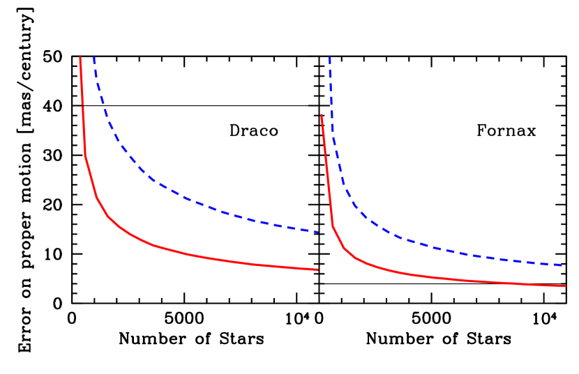
Figure 1.— The projected errors on the proper motion of dSphs as a function of the number of line-of-sight velocities, for two different models. The left panel uses the Draco fiducial model, while the right panel uses the Fornax fiducial model. In each panel, the solid (red) curve is for a non-rotating system, and the dashed (blue) curve includes a small rotational component. The lines indicate the approximate present errors on the proper motions. Measurement errors of 2 km s^-1 are assumed for line-of-sight velocities.

It is important to note that the projected errors in Figure 1 are valid only for the spatial distributions of stars and the measurement errors that we consider. The true constraints will depend on the detailed distributions of these quantities, and may in fact be reduced with more precise velocity measurements or varying stellar spatial distributions. For example, using the sample of Fornax red giants greater than 20th magnitude, we find sensitivities reduce to $\sim 3$ mas per century.

5. Contribution from Intrinsic Rotation

In the analysis above, we have assumed a negligible contribution from the intrinsic rotation in dSphs. This is a good model for the majority of these systems, which exhibit no detectable rotational or streaming motions in the kinematic data (Walker et al., 2006; Koch et al., 2007) (See however the recent results of  Battaglia et al. (2008), which show that rotation may be present in Sculptor).

Though the intrinsic rotation in dSphs is small, it is important to determine how even a small signal may degrade the constraints on the proper motions we have determined above. Probably the simplest rotational model to consider is a sinusoidal variation in the rotational velocity as a function of azimuthal angle (Drukier et al., 1998). In this model, a term of the form $A\sin(\phi_{i}+\phi_{0})$ can then be added to equation 1, where $A$ is the amplitude of the rotational motion, and $\phi_{0}$ is the projected axis about which the rotation occurs. We note that higher order multipoles may exist in the velocity field as a result of more complicated rotation or tidal effects; however here we assume these higher order terms are sub-dominant to the leading dipole term.

We add the parameters $A$ and $\phi_{0}$ to the Fisher matrix, and marginalize over them with uniform priors. In Figure 1, we show the projected proper motion errors including the effect of intrinsic rotation. Accounting for intrinsic rotation, we find that the errors on the proper motions may increase by about a factor of two for a fixed number of stars. Again, the details of the constraints depend on the exact distribution of the stars. Regarding the rotational parameters themselves, we find that $\phi_{0}$ is not well-constrained, but $A$ is determined to a precision of $\mathrel{\hbox{\hbox to0.0pt{\hbox{\lower 4.0pt\hbox{$\sim$}}\hss}\hbox{$<$}}}1$ km s^-1 with $\mathrel{\hbox{\hbox to0.0pt{\hbox{\lower 4.0pt\hbox{$\sim$}}\hss}\hbox{$>$}}}500$ line-of-sight velocities. Similar to $v_{x}$ and $v_{y}$, these errors on $A$ are independent of its mean value. We note that for Draco and Fornax the data suggest $A<1$ km s^-1.

We reiterate that our parametrization of rotation is a toy model introduced to understand the effect of including rotation on the precision with which proper motion may be measured. Although we have determined the errors on $A$ by solving for $\sigma_{los}$ using the Jeans equation, this procedure is not self-consistent, because in the presence of rotation the Jeans equation itself must be modified. In a rotating system, this would be important for determining the parameters describing the halo or the velocity anisotropy. However, since here we are interested only in determining the velocity components, all that we demand is $\sigma_{los}$ have enough freedom at each projected position to fit the kinematic data. As long as the streaming motion is small, as in the case of the dSphs we consider, this procedure should provide a good approximation to the errors on the model parameters $v_{x}$, $v_{y}$, $v_{z}$, and $A$.

6. Conclusions

We have shown that line-of-sight velocities from dwarf spheroidals can determine the transverse velocities of these galaxies to a precision of $\mathrel{\hbox{\hbox to0.0pt{\hbox{\lower 4.0pt\hbox{$\sim$}}\hss}\hbox{$<$}}}100$ km s^-1. This measurement utilizes “perspective rotation,” or the variation of the line-of-sight velocity across the galaxy resulting from its proper motion. The above sensitivity is similar to the current measurements from HST and ground-based imaging for dSphs such as Fornax, Carina, and Sculptor. Using perspective rotation, the proper motion errors for several dSphs, including Draco, will be reduced by at least a factor of two, and proper motions for dSphs such as Sextans, Leo I, and Leo II will be determined for the first time. We find that, with $\sim 10^{3}$ stars, the proper motion of Sextans can be determined to a sensitivity of $\sim 5$ mas per century, while for Leo I and Leo II we project errors of $\sim 10$ mas per century with $10^{3}$ stars.

Prospects are promising for improving on these measurements with future, larger samples of line-of-sight velocities. For example, we project that with $\sim 10^{4}$ line-of-sight velocities from Fornax, the errors are reduced by $\sim$ 40%. Proposed thirty meter class telescopes, such as the Thirty Meter Telescope (TMT) (http://www.tmt.org) and the Giant Magellan Telescope (GMT) (http://www.gmto.org), may measure velocities for $\sim 10^{4}$ stars in multiple dSphs, obtaining milli-arcsecond per century sensitivity. Nearby ultra-faint dwarfs, with extent $\sim 100$ pc and distances $\mathrel{\hbox{\hbox to0.0pt{\hbox{\lower 4.0pt\hbox{$\sim$}}\hss}\hbox{$<$}}}50$ kpc (Coma Berenices, Willman 1, Ursa Major II), may also be studied. In these objects we project errors $\sim 100$ mas per century with the optimistic scenario of $\sim 10^{3}$ stars.

A determination of dSph proper motions will provide a full three-dimensional mapping of their orbits, with prospects of improving the measurement of the Milky Way dark matter halo mass (Little & Tremaine, 1987). In addition, the proper motions will allow for a detailed comparison to the orbital properties of dark matter subhalos in numerical simulations (Diemand et al., 2007), and provide information on the merger and accretion histories of these satellites. It will be possible to determine which of the satellites are bound to the Milky Way, a property that may be closely intertwined with the complex star formation histories of several satellites  (Besla et al., 2007; Mateo et al., 2008).

7. Acknowledgments

We are grateful to Matt Walker for several important discussions, and for providing us with positions of Fornax red giants. We thank Betsy Barton, James Bullock, Jeff Cooke, Marla Geha, Josh Simon, and Beth Willman for discussions and encouragement. We acknowledge support from NSF grant AST-0607746.

References

- Battaglia et al. (2008) Battaglia, G., Helmi, A., Tolstoy, E., Irwin, M., Hill, V., & Jablonka, P. 2008, ArXiv e-prints, 802
- Besla et al. (2007) Besla, G., Kallivayalil, N., Hernquist, L., Robertson, B., Cox, T. J., van der Marel, R. P., & Alcock, C. 2007, ApJ, 668, 949
- Binney & Tremaine (1987) Binney, J. & Tremaine, S. 1987, Galactic Dynamics (Princeton: Princeton University Press)
- Diemand et al. (2007) Diemand, J., Kuhlen, M., & Madau, P. 2007, Astrophys. J., 657, 262
- Drukier et al. (1998) Drukier, G. A., Slavin, S. D., Cohn, H. N., Lugger, P. M., Berrington, R. C., Murphy, B. W., & Seitzer, P. O. 1998, AJ, 115, 708
- Feast et al. (1961) Feast, M. W., Thackeray, A. D., & Wesselink, A. J. 1961, MNRAS, 122, 433
- Gilmore et al. (2007) Gilmore, G., Wilkinson, M. I., Wyse, R. F. G., Kleyna, J. T., Koch, A., Evans, N. W., & Grebel, E. K. 2007, ApJ, 663, 948
- Gould (2000) Gould, A. 2000, ApJ, 528, 156
- Irwin & Hatzidimitriou (1995) Irwin, M. & Hatzidimitriou, D. 1995, MNRAS, 277, 1354
- Kendall & Stuart (1969) Kendall, M. G. & Stuart, A. 1969, The Advanced Theory of Statistics (London: Griffin)
- King (1962) King, I. 1962, AJ, 67, 471
- Koch et al. (2007) Koch, A., Kleyna, J. T., Wilkinson, M. I., Grebel, E. K., Gilmore, G. F., Evans, N. W., Wyse, R. F. G., & Harbeck, D. R. 2007, AJ, 134, 566
- Little & Tremaine (1987) Little, B. & Tremaine, S. 1987, ApJ, 320, 493
- Łokas et al. (2005) Łokas, E. L., Mamon, G. A., & Prada, F. 2005, MNRAS, 363, 918
- Mateo et al. (2008) Mateo, M., Olszewski, E. W., & Walker, M. G. 2008, ApJ, 675, 201
- Mateo (1998) Mateo, M. L. 1998, ARA&A, 36, 435
- Merritt et al. (1997) Merritt, D., Meylan, G., & Mayor, M. 1997, AJ, 114, 1074
- Piatek et al. (2005) Piatek, S., Pryor, C., Bristow, P., Olszewski, E. W., Harris, H. C., Mateo, M., Minniti, D., & Tinney, C. G. 2005, AJ, 130, 95
- Piatek et al. (2006) —. 2006, AJ, 131, 1445
- Piatek et al. (2007) —. 2007, AJ, 133, 818
- Scholz & Irwin (1994) Scholz, R.-D. & Irwin, M. J. 1994, in IAU Symposium, Vol. 161, Astronomy from Wide-Field Imaging, ed. H. T. MacGillivray, 535–+
- Simon & Geha (2007) Simon, J. D. & Geha, M. 2007, ApJ, 670, 313
- Strigari et al. (2007) Strigari, L. E., Bullock, J. S., Kaplinghat, M., Diemand, J., Kuhlen, M., & Madau, P. 2007, ApJ, 669, 676
- Strigari et al. (2007) Strigari, L. E., Koushiappas, S. M., Bullock, J. S., & Kaplinghat, M. 2007, Phys. Rev., D75, 083526
- Unwin et al. (2008) Unwin, S. C. et al. 2008, PASP, 120, 38
- van der Marel & Guhathakurta (2007) van der Marel, R. P. & Guhathakurta, P. 2007, ArXiv e-prints, 709
- Walker et al. (2006) Walker, M. G., Mateo, M., Olszewski, E. W., Bernstein, R., Wang, X., & Woodroofe, M. 2006, AJ, 131, 2114
- Walker et al. (2007) Walker, M. G., Mateo, M., Olszewski, E. W., Gnedin, O. Y., Wang, X., Sen, B., & Woodroofe, M. 2007, ApJ, 667, L53