Green function techniques
in the treatment of quantum transport
at the molecular scale

Abstract

The theoretical investigation of charge (and spin) transport at nanometer length scales requires the use of advanced and powerful techniques able to deal with the dynamical properties of the relevant physical systems, to explicitly include out-of-equilibrium situations typical for electrical/heat transport as well as to take into account interaction effects in a systematic way. Equilibrium Green function techniques and their extension to non-equilibrium situations via the Keldysh formalism build one of the pillars of current state-of-the-art approaches to quantum transport which have been implemented in both model Hamiltonian formulations and first-principle methodologies. In this chapter we offer a tutorial overview of the applications of Green functions to deal with some fundamental aspects of charge transport at the nanoscale, mainly focusing on applications to model Hamiltonian formulations.

1 Introduction

The natural limitations that are expected to arise by the further miniaturization attempts of semiconductor-based electronic devices have led in the past two decades to the emergence of the new field of molecular electronics, where electronic functions are going to be performed at the single-molecule level, see recent overview in Refs. Reed00sciam ; Joachim00nature ; Ratner02matertoday ; Nitzan03science ; Cuniberti05book ; Joachim05pnas . The original conception which lies at the bottom of this fascinating field can be traced back to the paper by Ari Aviram and Mark Ratner in 1974 Aviram74cpl , where a single-molecule rectifying diode was proposed. Obviously, one of the core issues at stake in molecular electronics is to clarify the question whether single molecules (or more complex molecular aggregates) can support an electric current. To achieve this goal, extremely refined experimental techniques are required in order to probe the response of such a nano-object to external fields. The meanwhile paradigmatic situation is that of a single molecule contacted by two metallic electrodes between which a bias voltage is applied.

Recent experiments

Enormous progress has been achieved in the experimental realization of such nano-devices, we only mention the development of controllable single-molecule junctions Reed97science -Loertscher07prl and scanning tunneling microscopy based techniques Porath97prb -Liljeroth07science . With their help, a plethora of interesting phenomena like rectification Elbing05pnas , negative differential conductance Chen99science ; Repp05prl , Coulomb blockade Porath97prb ; Park00nature ; Park02nature ; Yu04nanolett ; Yu04prl ; Osorio07advmat , Kondo effect Park02nature ; Liang02nature , vibrational effects Park00nature ; Hahn01prl ; Smit02nature ; Kushmerick04nanolett ; Yu04prl ; Liu04jcp ; Qiu04prl ; Wu04prl ; Repp05prl ; Repp05prl2 ; Osorio07advmat , and nanoscale memory effects Repp04science ; Choi06prl ; Martin06prl ; Olsson07prl ; Liljeroth07science , among others, have been demonstrated.

The traditional semiconductor nanoelectronics also remains in front of modern research, in particular due to recent experiments with small quantum dots, where cotunneling effects were observed Schleser05prl ; Sigrist06prl ; Sigrist07prl , as well as new rectification effects in double quantum dots, interpreted as spin blockade Ono02science ; Johnson05prb ; Muralidharan07prb ; Inarrea07prb . Note, that semiconductor experiments are very well controlled at present time, so they play an important role as a benchmark for the theory.

Apart from single molecules, carbon nanotubes have also found extensive applications and have been the target of experimental and theoretical studies over the last years, see Ref. Charlier07rmp for a very recent review. The expectations to realize electronics at the molecular scale also reached into the domain of bio-molecular systems, thus opening new perspectives for the field due to the specific self-recognition and self-assembling properties of biomolecules. For instance, DNA oligomers have been already used as templates in molecular electronic circuits Richter01apl ; Mertig02nanolett ; Keren03science . Much less clear is, however, if bio-molecules, and more specifically short DNA oligomers could also act as wiring systems. Their electrical response properties are much harder to disclose and there is still much controversy about the factors that determine charge migration through such systems Meggers98jacs ; Kelley99science ; Porath00nature ; Treadway02chemphys ; Xu04nanolett ; Gutierrez06inbook1 ; Gutierrez06inbook2 ; Porath04topics ; Shapir08nature .

Theoretical methods

The theoretical treatment of transport at the nanoscale (see introduction in Datta95book ; Haug96book ; Ferry97book ; Dittrich98book ; Bruus04book ; Datta05book ) requires the combined use of different techniques which range from minimal model Hamiltonians, passing through semi-empirical methods up to full first-principle methodologies. We mention here some important contributions, while we have no possibility to cite all relevant papers.

Model Hamiltonians can in a straightforward way select, out of the many variables that can control charge migration those which are thought to be the most relevant ones for a specific molecule-electrode set-up. They contain, however, in a sometimes not well-controlled way, many free parameters; hence, they can point at generic effects, but they must be complemented with other methodologies able to yield microscopic specific information. Semi-empirical methods can deal with rather large systems due to the use of special subsets of electronic states to construct molecular Hamiltonians as well as to the approximate treatment of interactions, but often have the drawback of not being transferable. Ab initio approaches, finally, can deal in a very precise manner with the electronic and atomic structure of the different constituents of a molecular junction (metallic electrodes, molecular wire, the interface) but it is not apriori evident that they can also be applied to strong non-equilibrium situations.

From a more formal standpoint, there are roughly two main theoretical frameworks that can be used to study quantum transport in nanosystems at finite voltage: generalized master equations (GME) Weiss99book ; Breuer02book and nonequilibrium Green function (NGF) techniques Kadanoff62book ; Keldysh64 ; Langreth76inbook ; Rammer86RMP ; Haug96book . The former also lead to more simple rate equations in the case where (i) the electrode-system coupling can be considered as a weak perturbation, and (ii) off-diagonal elements of the reduced density matrix in the eigenstate representation (coherences) can be neglected due to very short decoherence times. Both approaches, the GME and NGF techniques, can yield formally exact expressions for many observables. For non-interacting systems, one can even solve analytically many models. However, once interactions are introduced - and these are the most interesting cases containing a very rich physics - different approximation schemes have to be introduced to make the problems tractable.

In this chapter, we will review mainly the technique of non-equilibrium Green functions. This approach is able to deal with a very broad variety of physical problems related to quantum transport at the molecular scale. It can deal with strong non-equilibrium situations via an extension of the conventional GF formalism to the Schwinger-Keldysh contour Keldysh64 and it can also include interaction effects (electron-electron, electron-vibron, etc) in a systematic way (diagrammatic perturbation theory, equation of motion techniques). Proposed first time for the mesoscopic structures in the early seventies by Caroli et al. Caroli71jpcss1 ; Caroli71jpcss2 ; Caroli71jpcss3 ; Caroli71jpcss4 , this approach was formulated in an elegant way by Meir, Wingreen and Jauho Meir92prl ; Wingreen93prb ; Jauho94prb ; Haug96book ; Jauho06jpcs , who derived exact expression for nonequilibrium current through an interacting nanosystem placed between large noninteracting leads in terms of the nonequilibrium Green functions of the nanosystem. Still, the problem of calculation of these Green functions is not trivial. We consider some possible approaches in the case of electron-electron and electron-vibron interactions. Moreover, as we will show later on, it can reproduce results obtained within the master equation approach in the weak coupling limit to the electrodes (Coulomb blockade), but it can also go beyond this limit and cover intermediate coupling (Kondo effect) and strong coupling (Fabry-Perot) domains. It thus offer the possibility of dealing with different physical regimes in a unified way.

Now we review briefly some results obtained recently in the main directions of modern research: general nanoscale quantum transport theory, atomistic transport theory and applications to particular single-molecule systems.

General nanoscale quantum transport theory

On the way to interpretation of modern experiments with single-molecule junctions and STM spectroscopy of single molecules on surfaces, two main theoretical problems are to be solved. The first is development of appropriate models based on ab initio formulation. The second is effective and scalable theory of quantum transport through multilevel interacting systems. We first consider the last problem, assuming that the model Hamiltonian is known. Quantum transport through noninteracting system can be considered using the famous Landauer-Büttiker method Landauer57ibm ; Landauer70philmag ; Economou81prl ; FisherLee81prb ; Buttiker85prb ; Buttiker86prl ; Landauer88ibm ; Buttiker88ibm ; Stone88ibm ; Baranger89prb , which establishes the fundamental relation between the wave functions (scattering amplitudes) of a system and its conducting properties. The method can be applied to find the current through a noninteracting system or through an effectively noninteracting system, for example if the mean-field description is valid and the inelastic scattering is not essential. Such type of an electron transport is called coherent, because there is no phase-breaking and quantum interference is preserved during the electron motion across the system. In fact, coherence is initially assumed in many ab initio based transport methods (DFT+NGF, and others), so that the Landauer-Büttiker method is now routinely applied to any basic transport calculation through nanosystems and single molecules. Besides, it is directly applicable in many semiconductor quantum dot systems with weak electron-electron interactions. Due to simplicity and generality of this method, it is now widely accepted and is in the base of our understanding of coherent transport.

However, the peculiarity of single-molecule transport is just essential role of electron-electron and electron-vibron interactions, so that Landauer-Büttiker method is not enough usually to describe essential physics even qualitatively. During last years many new methods were developed to describe transport at finite voltage, with focus on correlation and inelastic effects, in particular in the cases when Coulomb blockade, Kondo effect and vibronic effects take place.

Vibrons (the localized phonons) are very important because molecules are flexible. The theory of electron-vibron interaction has a long history, but many questions it implies are not answered up to now. While the isolated electron-vibron model can be solved exactly by the so-called polaron or Lang-Firsov transformation Lang63jetp ; Hewson74jjap ; Mahan90book , the coupling to the leads produces a true many-body problem. The inelastic resonant tunneling of single electrons through the localized state coupled to phonons was considered in Refs. Glazman88jetp ; Wingreen88prl ; Wingreen89prb ; Jonson89prb ; Cizek04prb ; Cizek05czechjp . There the exact solution in the single-particle approximation was derived, ignoring completely the Fermi sea in the leads. At strong electron-vibron interaction and weak couplings to the leads the satellites of the main resonant peak are formed in the spectral function.

The essential progress in calculation of transport properties in the strong electron-vibron interaction limit has been made with the help of the master equation approach Braig03prb ; Aji03condmat ; Mitra04prb ; Koch05prl ; Koch06prb ; Koch06prb2 ; Wegewijs05condmat ; Zazunov06prb1 ; Ryndyk08preprint . This method, however, is valid only in the limit of very weak molecule-to-lead coupling and neglects all spectral effects, which are the most important at finite coupling to the leads.

At strong coupling to the leads and the finite level width the master equation approach can no longer be used, and we apply alternatively the nonequilibrium Green function technique which have been recently developed to treat vibronic effects in a perturbative or self-consistent way in the cases of weak and intermediate electron-vibron interaction Tikhodeev01surfsci ; Mii02surfsci ; Mii03prb ; Tikhodeev04prb ; Galperin04nanolett ; Galperin04jcp ; Galperin05jphyschemb ; Frederiksen04master ; Frederiksen04prl ; Hartung04master ; Ryndyk05prb ; Ryndyk06prb ; Ryndyk07prb ; Paulsson05prb ; Paulsson06jpconf ; Arseyev05jetplett ; Arseyev06jetplett ; Zazunov06prb .

The case of intermediate and strong electron-vibron interaction at intermediate coupling to the leads is the most interesting, but also the most difficult. The existing approaches are mean-field Hewson79jphysc ; Galperin05nanolett ; DAmico08njp , or start from the exact solution for the isolated system and then treat tunneling as a perturbation Kral97 ; Lundin02prb ; Zhu03prb ; Alexandrov03prb ; Flensberg03prb ; Galperin06prb ; Zazunov07prb . The fluctuations beyond mean-field approximations were considered in Refs.  Mitra05prl ; Mozyrsky06prb

In parallel, the related activity was in the field of single-electron shuttles and quantum shuttles Gorelik98prl ; Boese01epl ; Fedorets02epl ; Fedorets03prb ; Fedorets04prl ; McCarthy03prb ; Novotny03prl ; Novotny04prl ; Blanter04prl ; Smirnov04prb ; Chtchelkatchev04prb . Finally, based on the Bardeen’s tunneling Hamiltonian method Bardeen61prl ; Harrison61pr ; Cohen62prl ; Prange63pr ; Duke69book and Tersoff-Hamann approach Tersoff83prl ; Tersoff85prb , the theory of inelastic electron tunneling spectroscopy (IETS) was developed Persson87prl ; Gata93prb ; Tikhodeev01surfsci ; Mii02surfsci ; Mii03prb ; Tikhodeev04prb ; Raza07condmat .

The recent review of the electron-vibron problem and its relation to the molecular transport see in Ref. Galperin07jpcm .

Coulomb interaction is the other important ingredient of the models, describing single molecules. It is in the origin of such fundamental effects as Coulomb blockade and Kondo efect. The most convenient and simple enough is Anderson-Hubbard model, combining the formulations of Anderson impurity model Anderson61prev and Hubbard many-body model Hubbard63procroysoc ; Hubbard64procroysoc1 ; Hubbard64procroysoc2 . To analyze such strongly correlated system several complementary methods can be used: master equation and perturbation in tunneling, equation-of-motion method, self-consistent Green functions, renormalization group and different numerical methods.

When the coupling to the leads is weak, electron-electron interaction results in Coulomb blockade, the sequential tunneling is described by the master equation method Averin86jltp ; Averin91inbook ; Grabert92book ; vanHouten92inbook ; Kouwenhoven97inbook ; Schoeller97inbook ; Schoen97inbook ; vanderWiel02rmp and small cotunneling current in the blockaded regime can be calculated by the next-order perturbation theory Averin89pla ; Averin90prl ; Averin92inbook . This theory was used successfully to describe electron tunneling via discrete quantum states in quantum dots Averin91prb ; Beenakker91prb ; vonDelft01pr ; Bonet02prb . Recently there were several attempts to apply master equation to multi-level models of molecules, in particular describing benzene rings Hettler03prl ; Muralidharan06prb ; Begemann08prb .

To describe consistently cotunneling, level broadening and higher-order (in tunneling) processes, more sophisticated methods to calculate the reduced density matrix were developed, based on the Liouville - von Neumann equation Petrov04chemphys ; Petrov05chemphys ; Petrov06prb ; Elste05prb ; Harbola06prb ; Pedersen07prb ; Mayrhofer07epjb ; Begemann08prb or real-time diagrammatic technique Schoeller94prb ; Koenig96prl ; Koenig96prb ; Koenig97prl ; Koenig98prb ; Thielmann03prb ; Thielmann05prl ; Aghassi06prb . Different approaches were reviewed recently in Ref. Timm08prb .

The equation-of-motion (EOM) method is one of the basic and powerful ways to find the Green functions of interacting quantum systems. In spite of its simplicity it gives the appropriate results for strongly correlated nanosystems, describing qualitatively and in some cases quantitatively such important transport phenomena as Coulomb blockade and Kondo effect in quantum dots. The results of the EOM method could be calibrated with other available calculations, such as the master equation approach in the case of weak coupling to the leads, and the perturbation theory in the case of strong coupling to the leads and weak electron-electron interaction.

In the case of a single site junction with two (spin-up and spin-down) states and Coulomb interaction between these states (Anderson impurity model), the linear conductance properties have been successfully studied by means of the EOM approach in the cases related to Coulomb blockadeLacroix81jphysf ; Meir91prl and the Kondo effect Meir93prl . Later the same method was applied to some two-site models Niu95prb ; Pals96jpcm ; Lamba00prb ; Song07prb . Multi-level systems were started to be considered only recently Palacios97prb ; Yi02prb . Besides, there are some difficulties in building the lesser GF in the nonequilibrium case (at finite bias voltages) by means of the EOM method Niu99jpcm ; Swirkowicz03prb ; Bulka04prb .

The diagrammatic method was also used to analyze the Anderson impurity model. First of all, the perturbation theory can be used to describe weak electron-electron interaction and even some features of the Kondo effect Fujii03prb . The family of nonperturbative current-conserving self-consistent approximations for Green functions has a long history and goes back to the Schwinger functional derivative technique, Kadanoff-Baym approximations and Hedin equations in the equilibrium many-body theory Schwinger51pnas ; Martin59prev ; Baym61prev ; Baym62prev ; Hedin65prev ; Gunnarsson88rpp ; White92prb ; Onida02rmp . Recently GW approximation was investigated together with other methods Thygesen07jcp ; Thygesen08prl ; Thygesen08prb ; Wang08prb . It was shown that dynamical correlation effects and self-consistency can be very important at finite bias.

Finally, we want to mention briefly three important fields of research, that we do not consider in the present review: the theory of Kondo effect Glazman88jetplett ; Ng88prl ; Hershfield92prb ; Meir93prl ; Wingreen94prb ; Aguado00prl ; Kim01prb ; Plihal01prb , spin-dependent transport Sanvito06jctn ; Rocha06prb ; Naber07jpdap ; Ke08prl ; Ning08prl , and time-dependent transport Jauho94prb ; Grifoni98pr ; Kohler05pr ; Sanchez06prb ; Maciejko06prb .

Atomistic transport theory

Atomistic transport theory utilizes semi-empirical (tight-binding Cuniberti02cp ; Todorov02jpcm ) or ab initio based methods. In all cases the microscopic structure is taken into account with different level of accuracy.

The most popular is the approach combining density-functional theory (DFT) and NGF and known as DFT+NGF Taylor01prb1 ; Taylor01prb2 ; Damle01prb ; Xue01jcp ; Xue02cp ; Xue03prb1 ; Xue03prb2 ; DiCarlo02pb ; Frauenheim02jpcm ; Brandbyge02prb ; Taylor03prb ; Lee04prb ; Pecchia04repprogphys ; Ke04prb ; Ke05prb ; Ke05jcp1 ; Ke05jcp2 ; Liu06jcp ; Ke07jcp ; Pump07ss ; DelValle07naturenanotech ; Pecchia07prb ; Pecchia08njp . This method, however is not free from internal problems. First of all, it is essentially mean-filed method neglecting strong local correlations and inelastic scattering. Second, density-functional theory is a ground state theory and e.g. the transmission calculated using static DFT eigenvalues will display peaks at the Kohn-Sham excitation energies, which in general do not coincide with the true excitation energies. Extensions to include excited states as in time-dependent density-functional theory, though very promising Sai05prl ; Kurth05prb ; DiVentra07prl , are not fully developed up to date.

To improve DFT-based models several approaches were suggested, including inelastic electron-vibron interaction Frederiksen04prl ; Pecchia04nanolett ; Sergueev05prl ; Paulsson05prb ; Paulsson06nanolett ; Frederiksen07prb ; Frederiksen07prb2 ; Gagliardi08njp ; Raza08condmat ; Raza08prb or Coulomb interaction beyond mean-field level Ferretti05prb , or based on the LDA+U approache Anisimov91prb . The principally different alternative to DFT is to use an initio quantum chemistry based many-body quantum transport approach Delaney04prl ; Delaney04intjquantumchem ; Fagas06prb ; Albrecht06jap .

Finally, transport in bio-molecules attracted more attention, in particular electrical conductance of DNA Cuniberti02prb ; Gutierrez03eurolett ; Gutierrez05nanolett ; Gutierrez05prb ; Gutierrez06prb .

Outline

The review is organized as follows. In Sections 2 we will first introduce the Green functions for non-interacting systems, and present few examples of transport through non-interacting regions. Then we review the master equation approach and its application to describe Coulomb blockade and vibron-mediated Franck-Condon blockade. In Section 3 the Keldysh NGF technique is developed in detail. In equilibrium situations or within the linear response regime, dynamic response and static correlation functions are related via the fluctuation-dissipation theorem. Thus, solving Dyson equation for the retarded GF is enough to obtain the correlation functions. In strong out-of-equilibrium situations, however, dynamic response and correlation functions have to be calculated simultaneously and are not related by fluctuation-dissipation theorems. The Kadanof-Baym-Keldysh approach yield a compact, powerful formulation to derive Dyson and kinetic equations for non-equilibrium systems. In Sec. 4 we present different applications of the Green function techniques. We show how Coulomb blockade can be described within the Anderson-Hubbard model, once an appropriate truncation of the equation of motion hierarchy is performed (Sec. 4.A). Further, the paradigmatic case of transport through a single electronic level coupled to a local vibrational mode is discussed in detail within the context of the self-consistent Born approximation. It is shown that already this simple model can display non-trivial physics (Sec. 4.B). Finally, the case of an electronic system interacting with a bosonic bath is discussed in Sec. 4.C where it is shown that the presence of an environment with a continuous spectrum can modified the low-energy analytical structure of the Green function and lead to dramatic changes in the electrical response of the system. We point at the relevance of this situation to discuss transport experiments in short DNA oligomers. We have not addressed the problem of the (equilibrium or non-equilibrium) Kondo effect, since this issue alone would require a chapter on its own due to the non-perturbative character of the processes leading to the formation of the Kondo resonance.

In view of the broadness of the topic, the authors were forced to do a very subjective selection of the topics to be included in this review as well as of the most relevant literature. We thus apologize for the omission of many interesting studies which could not be dealt with in the restricted space at our disposal. We refer the interested reader to the other contributions in this book and the cited papers.

2 From coherent transport to sequential tunneling (basics)

2.1 Coherent transport: single-particle Green functions

Nano-scale and molecular-scale systems are naturally described by the discrete-level models, for example eigenstates of quantum dots, molecular orbitals, or atomic orbitals. But the leads are very large (infinite) and have a continuous energy spectrum. To include the lead effects systematically, it is reasonable to start from the discrete-level representation for the whole system. It can be made by the tight-binding (TB) model, which was proposed to describe quantum systems in which the localized electronic states play an essential role, it is widely used as an alternative to the plane wave description of electrons in solids, and also as a method to calculate the electronic structure of molecules in quantum chemistry.

A very effective method to describe scattering and transport is the Green function (GF) method. In the case of non-interacting systems and coherent transport single-particle GFs are used. In this section we consider the matrix Green function method for coherent transport through discrete-level systems.

(i) Matrix (tight-binding) Hamiltonian

The main idea of the method is to represent the wave function of a particle as a linear combination of some known localized states $\psi_{\alpha}({\bf r},\sigma)$, where $\alpha$ denote the set of quantum numbers, and $\sigma$ is the spin index (for example, atomic orbitals, in this particular case the method is called LCAO – linear combination of atomic orbitals)

$$\psi(\xi)=\sum_{\alpha}c_{\alpha}\psi_{\alpha}(\xi),$$ (1)

here and below we use $\xi\equiv(\bf r,\sigma)$ to denote both spatial coordinates and spin.

Using the Dirac notations $|\alpha\rangle\equiv\psi_{\alpha}(\xi)$ and assuming that $\psi_{\alpha}(\xi)$ are orthonormal functions $\langle\alpha|\beta\rangle=\delta_{\alpha\beta}$ we can write the single-particle matrix (tight-binding) Hamiltonian in the Hilbert space formed by $\psi_{\alpha}(\xi)$

$$\hat{H}=\sum_{\alpha}(\epsilon_{\alpha}+e\varphi_{\alpha})|\alpha\rangle\langle\alpha|+\sum_{\alpha\beta}t_{\alpha\beta}|\alpha\rangle\langle\beta|,$$ (2)

the first term in this Hamiltonian describes the states with energies $\epsilon_{\alpha}$, $\varphi_{\alpha}$ is the electrical potential, the second term should be included if the states $|\alpha\rangle$ are not eigenstates of the Hamiltonoian. In the TB model $t_{\alpha\beta}$ is the hopping matrix element between states $|\alpha\rangle$ and $|\beta\rangle$, which is nonzero, as a rule, for nearest neighbor cites. The two-particle interaction is described by the Hamiltonian

$$\hat{H}=\sum_{\alpha\beta,\delta\gamma}V_{\alpha\beta,\delta\gamma}|\alpha\rangle|\beta\rangle\langle\delta|\langle\gamma|,$$ (3)

in the two-particle Hilbert space, and so on.

The energies and hopping matrix elements in this Hamiltomian can be calculated, if the single-particle real-space Hamiltomian $\hat{h}(\xi)$ is known:

$$\epsilon_{\alpha}\delta_{\alpha\beta}+t_{\alpha\beta}=\int\psi^{*}_{\alpha}(\xi)\hat{h}(\xi)\psi_{\beta}(\xi)d\xi.$$ (4)

This approach was developed originally as an approximate method, if the wave functions of isolated atoms are taken as a basis wave functions $\psi_{\alpha}(\xi)$, but also can be formulated exactly with the help of Wannier functions. Only in the last case the expansion (1) and the Hamiltonian (2) are exact, but some extension to the arbitrary basis functions is possible. In principle, the TB model is reasonable only when local states can be orthogonalized. The method is useful to calculate the conductance of complex quantum systems in combination with ab initio methods. It is particular important to describe small molecules, when the atomic orbitals form the basis.

In the mathematical sense, the TB model is a discrete (grid) version of the continuous Schrödinger equation, thus it is routinely used in numerical calculations.

To solve the single-particle problem it is convenient to introduce a new representation, where the coefficients $c_{\alpha}$ in the expansion (1) are the components of a vector wave function (we assume here that all states $\alpha$ are numerated by integers)

$$\Psi=\left(\begin{array}[]{c}c_{1}\\ c_{2}\\ \vdots\\ c_{N}\end{array}\right),$$ (5)

and the eigenstates $\Psi_{\lambda}$ are to be found from the matrix Schrödinger equation

$${\bf H}\Psi_{\lambda}=E_{\lambda}\Psi_{\lambda},$$ (6)

with the matrix elements of the single-particle Hamiltonian

$$H_{\alpha\beta}=\left\{\begin{array}[]{ll}\epsilon_{\alpha}+e\varphi_{\alpha},&\alpha=\beta,\\ t_{\alpha\beta},&\alpha\neq\beta.\end{array}\right.$$ (7)

Figure 1: A finite linear chain of single-level sites.

Now let us consider some typical systems, for which the matrix method is appropriate starting point. The simplest example is a single quantum dot, the basis is formed by the eigenstates, the corresponding Hamiltonian is diagonal

$${\bf H}=\left(\begin{array}[]{ccccc}\epsilon_{1}&0&0&\cdots&0\\ 0&\epsilon_{2}&0&\cdots&0\\ \vdots&\ddots&\ddots&\ddots&\vdots\\ 0&\cdots&0&\epsilon_{N-1}&0\\ 0&\cdots&0&0&\epsilon_{N}\end{array}\right).$$ (8)

The next typical example is a linear chain of single-state sites with only nearest-neighbor couplings (Fig. 1)

$${\bf H}=\left(\begin{array}[]{ccccc}\epsilon_{1}&t&0&\cdots&0\\ t&\epsilon_{2}&t&\cdots&0\\ \vdots&\ddots&\ddots&\ddots&\vdots\\ 0&\cdots&t&\epsilon_{N-1}&t\\ 0&\cdots&0&t&\epsilon_{N}\end{array}\right).$$ (9)

The method is applied as well to consider the semi-infinite leads. Although the matrices are formally infinitely-dimensional in this case, we shall show below, that the problem is reduced to the finite-dimensional problem for the quantum system of interest, and the semi-infinite leads can be integrated out.

Finally, in the second quantized form the tight-binding Hamiltonian is

$$\hat{H}=\sum_{\alpha}\left(\epsilon_{\alpha}+e\varphi_{\alpha}\right)c^{\dagger}_{\alpha}c_{\alpha}+\sum_{\alpha\neq\beta}t_{\alpha\beta}c^{\dagger}_{\alpha}c_{\beta}.$$ (10)

(ii) Matrix Green functions and contact self-energies

The solution of single-particle quantum problems, formulated with the help of a matrix Hamiltonian, is possible along the usual line of finding the wave-functions on a lattice, solving the Schrödinger equation (6). The other method, namely matrix Green functions, considered in this section, was found to be more convenient for transport calculations, especially when interactions are included.

The retarded single-particle matrix Green function ${\bf G}^{R}(\epsilon)$ is determined by the equation

$$\left[(\epsilon+i\eta){\bf I}-{\bf H}\right]{\bf G}^{R}={\bf I},$$ (11)

where $\eta$ is an infinitesimally small positive number $\eta=0^{+}$.

For an isolated noninteracting system the Green function is simply obtained after the matrix inversion

$${\bf G}^{R}=\left[(\epsilon+i\eta){\bf I}-{\bf H}\right]^{-1}.$$ (12)

Let us consider the trivial example of a two-level system with the Hamiltonian

$${\bf H}=\left(\begin{array}[]{cc}\epsilon_{1}&t\\ t&\epsilon_{2}\end{array}\right).$$ (13)

The retarded GF is easy found to be ($\tilde{\epsilon}=\epsilon+i\eta$)

$${\bf G}^{R}(\epsilon)=\frac{1}{(\tilde{\epsilon}-\epsilon_{1})(\tilde{\epsilon}-\epsilon_{2})+t^{2}}\left(\begin{array}[]{cc}\tilde{\epsilon}-\epsilon_{2}&t\\ t&\tilde{\epsilon}-\epsilon_{1}\end{array}\right).$$ (14)

Figure 2: A quantum system coupled to the left and right leads.

Now let us consider the case, when the system of interest is coupled to two contacts (Fig. 2). We assume here that the contacts are also described by the tight-binding model and by the matrix GFs. Actually, the semi-infinite contacts should be described by the matrix of infinite dimension. We shall consider the semi-infinite contacts in the next section.

Let us present the full Hamiltonian of the considered system in a following block form

$${\bf H}=\left(\begin{array}[]{ccc}{\bf H}^{0}_{L}&{\bf H}_{LS}&0\\ {\bf H}^{\dagger}_{LS}&{\bf H}^{0}_{S}&{\bf H}^{\dagger}_{RS}\\ 0&{\bf H}_{RS}&{\bf H}^{0}_{R}\end{array}\right),$$ (15)

where ${\bf H}^{0}_{L}$, ${\bf H}^{0}_{S}$, and ${\bf H}^{0}_{R}$ are Hamiltonians of the left lead, the system, and the right lead separately. And the off-diagonal terms describe system-to-lead coupling. The Hamiltonian should be hermitian, so that

$${\bf H}_{SL}={\bf H}^{\dagger}_{LS},\ \ \ {\bf H}_{SR}={\bf H}^{\dagger}_{RS}.$$ (16)

The Eq. (11) can be written as

$$\left(\begin{array}[]{ccc}{\bf E}-{\bf H}^{0}_{L}&-{\bf H}_{LS}&0\\ -{\bf H}^{\dagger}_{LS}&{\bf E}-{\bf H}^{0}_{S}&-{\bf H}^{\dagger}_{RS}\\ 0&-{\bf H}_{RS}&{\bf E}-{\bf H}^{0}_{R}\end{array}\right)\left(\begin{array}[]{ccc}{\bf G}_{L}&{\bf G}_{LS}&0\\ {\bf G}_{SL}&{\bf G}_{S}&{\bf G}_{SR}\\ 0&{\bf G}_{RS}&{\bf G}_{R}\end{array}\right)={\bf I},$$ (17)

where we introduce the matrix ${\bf E}=(\epsilon+i\eta){\bf I}$, and represent the matrix Green function in a convenient form, the notation of retarded function is omitted in intermediate formulas. Now our first goal is to find the system Green function ${\bf G}_{S}$ which defines all quantities of interest. From the matrix equation (17)

$$\left({\bf E}-{\bf H}^{0}_{L}\right){\bf G}_{LS}-{\bf H}_{LS}{\bf G}_{S}=0,$$ (18)

$$-{\bf H}^{\dagger}_{LS}{\bf G}_{LS}+\left({\bf E}-{\bf H}^{0}_{S}\right){\bf G}_{S}-{\bf H}^{\dagger}_{RS}{\bf G}_{RS}={\bf I},$$ (19)

$$-{\bf H}_{RS}{\bf G}_{S}+\left({\bf E}-{\bf H}^{0}_{R}\right){\bf G}_{RS}=0.$$ (20)

From the first and the third equations one has

$${\bf G}_{LS}=\left({\bf E}-{\bf H}^{0}_{L}\right)^{-1}{\bf H}_{LS}{\bf G}_{S},$$ (21)

$${\bf G}_{RS}=\left({\bf E}-{\bf H}^{0}_{R}\right)^{-1}{\bf H}_{RS}{\bf G}_{S},$$ (22)

and substituting it into the second equation we arrive at the equation

$$\left({\bf E}-{\bf H}^{0}_{S}-{\bf\Sigma}\right){\bf G}_{S}={\bf I},$$ (23)

where we introduce the contact self-energy (which should be also called retarded, we omit the index in this chapter)

$${\bf\Sigma}={\bf H}^{\dagger}_{LS}\left({\bf E}-{\bf H}^{0}_{L}\right)^{-1}{\bf H}_{LS}+{\bf H}^{\dagger}_{RS}\left({\bf E}-{\bf H}^{0}_{R}\right)^{-1}{\bf H}_{RS}.$$ (24)

Finally, we found, that the retarded GF of a nanosystem coupled to the leads is determined by the expression

$${\bf G}^{R}_{S}(\epsilon)=\left[(\epsilon+i\eta){\bf I}-{\bf H}^{0}_{S}-{\bf\Sigma}\right]^{-1},$$ (25)

the effects of the leads are included through the self-energy.

Here we should stress the important property of the self-energy (24), it is determined only by the coupling Hamiltonians and the retarded GFs of the isolated leads ${\bf G}^{0R}_{i}=\left({\bf E}-{\bf H}^{0}_{R}\right)^{-1}$ ($i=L,R$)

$${\bf\Sigma}_{i}={\bf H}^{\dagger}_{iS}\left({\bf E}-{\bf H}^{0}_{i}\right)^{-1}{\bf H}_{iS}={\bf H}^{\dagger}_{iS}{\bf G}^{0R}_{i}{\bf H}_{iS},$$ (26)

it means, that the contact self-energy is independent of the state of the nanosystem itself and describes completely the influence of the leads. Later we shall see that this property conserves also for interacting system, if the leads are noninteracting.

Finally, we should note, that the Green functions considered in this section, are single-particle GFs, and can be used only for noninteracting systems.

(iii) Semi-infinite leads

Let us consider now a nanosystem coupled to a semi-infinite lead (Fig. 3). The direct matrix inversion can not be performed in this case. The spectrum of a semi-infinite system is continuous. We should transform the expression (26) into some other form.

Figure 3: A quantum system coupled to a semi-infinite 1D lead.

To proceed, we use the relation between the Green function and the eigenfunctions $\Psi_{\lambda}$ of a system, which are solutions of the Schrödinger equation (6). Let us define $\Psi_{\lambda}(\alpha)\equiv c_{\lambda}$ in the eigenstate $|\lambda\rangle$ in the sense of definition (5), then

$$G^{R}_{\alpha\beta}(\epsilon)=\sum_{\lambda}\frac{\Psi_{\lambda}(\alpha)\Psi^{*}_{\lambda}(\beta)}{\epsilon+i\eta-E_{\lambda}},$$ (27)

where $\alpha$ is the TB state (site) index, $\lambda$ denotes the eigenstate, $E_{\lambda}$ is the energy of the eigenstate. The summation in this formula can be easy replaced by the integration in the case of a continuous spectrum. It is important to notice, that the eigenfunctions $\Psi_{\lambda}(\alpha)$ should be calculated for the separately taken semi-infinite lead, because the Green function of isolated lead is substituted into the contact self-energy.

For example, for the semi-infinite 1D chain of single-state sites ($n,m=1,2,...$)

$$G^{R}_{nm}(\epsilon)=\int_{-\pi}^{\pi}\frac{dk}{2\pi}\frac{\Psi_{k}(n)\Psi^{*}_{k}(m)}{\epsilon+i\eta-E_{k}},$$ (28)

with the eigenfunctions $\Psi_{k}(n)=\sqrt{2}\sin kn$, $E_{k}=\epsilon_{0}+2t\cos k$.

Let us consider a simple situation, when the nanosystem is coupled only to the end site of the 1D lead (Fig. 3). From (26) we obtain the matrix elements of the self-energy

$$\Sigma_{\alpha\beta}=V^{*}_{1\alpha}V_{1\beta}G^{0R}_{11},$$ (29)

where the matrix element $V_{1\alpha}$ describes the coupling between the end site of the lead ($n=m=1$) and the state $|\alpha\rangle$ of the nanosystem.

To make clear the main physical properties of the lead self-energy, let us analyze in detail the semi-infinite 1D lead with the Green function (28). The integral can be calculated analytically (Datta05book , p. 213, Cuniberti02cp )

$$G^{R}_{11}(\epsilon)=\frac{1}{\pi}\int_{-\pi}^{\pi}\frac{\sin^{2}kdk}{\epsilon+i\eta-\epsilon_{0}-2t\cos k}=-\frac{\exp(iK(\epsilon))}{t},$$ (30)

$K(\epsilon)$ is determined from $\epsilon=\epsilon_{0}+2t\cos K$. Finally, we obtain the following expressions for the real and imaginary part of the self-energy

$$\displaystyle{\rm Re}\Sigma_{\alpha\alpha}=\frac{|V_{1\alpha}|^{2}}{t}\left(\kappa-\sqrt{\kappa^{2}-1}\left[\theta(\kappa-1)-\theta(-\kappa-1)\right]\right),$$ (31)

$$\displaystyle{\rm Im}\Sigma_{\alpha\alpha}=-\frac{|V_{1\alpha}|^{2}}{t}\sqrt{1-\kappa^{2}}\theta(1-|\kappa|),$$ (32)

$$\displaystyle\kappa=\frac{\epsilon-\epsilon_{0}}{2t}.$$ (33)

The real and imaginary parts of the self-energy, given by these expressions, are shown in Fig. 4. There are several important general conclusion that we can make looking at the formulas and the curves.

(a) The self-energy is a complex function, the real part describes the energy shift of the level, and the imaginary part describes broadening. The finite imaginary part appears as a result of the continuous spectrum in the leads. The broadening is described traditionally by the matrix

$${\bf\Gamma}=i\left({\bf\Sigma}-{\bf\Sigma}^{\dagger}\right),$$ (34)

called level-width function.

(b) In the wide-band limit ($t\rightarrow\infty$), at the energies $\epsilon-\epsilon_{0}\ll t$, it is possible to neglect the real part of the self-energy, and the only effect of the leads is level broadening. So that the self-energy of the left (right) lead is

$${\bf\Sigma}_{L(R)}=-i\frac{{\bf\Gamma}_{L(R)}}{2}.$$ (35)

Figure 4: (Color) Real and imaginary parts of the contact self-energy as a function of energy for a one-band one-dimensional lead.

(iv) Transmission, conductance, current

After all, we want again to calculate the current through the nanosystem. We assume, as before, that the contacts are equilibrium, and there is the voltage $V$ applied between the left and right contacts. The calculation of the current in a general case is more convenient to perform using the full power of the nonequilibrium Green function method. Here we present a simplified approach, valid for noninteracting systems only, following Paulsson Paulsson02condmat .

Let us come back to the Schrödinger equation (6) in the matrix representation, and write it in the following form

$$\left(\begin{array}[]{ccc}{\bf H}^{0}_{L}&{\bf H}_{LS}&0\\ {\bf H}^{\dagger}_{LS}&{\bf H}^{0}_{S}&{\bf H}^{\dagger}_{RS}\\ 0&{\bf H}_{RS}&{\bf H}^{0}_{R}\end{array}\right)\left(\begin{array}[]{c}\Psi_{L}\\ \Psi_{S}\\ \Psi_{R}\end{array}\right)=E\left(\begin{array}[]{c}\Psi_{L}\\ \Psi_{S}\\ \Psi_{R}\end{array}\right),$$ (36)

where $\Psi_{L}$, $\Psi_{S}$, and $\Psi_{R}$ are vector wave functions of the left lead, the nanosystem, and the right lead correspondingly.

Now we find the solution in the scattering form (which is difficult to call true scattering because we do not define explicitly the geometry of the leads). Namely, in the left lead $\Psi_{L}=\Psi^{0}_{L}+\Psi^{1}_{L}$, where $\Psi^{0}_{L}$ is the eigenstate of ${\bf H}^{0}_{L}$, and is considered as known initial wave. The ”reflected” wave $\Psi^{1}_{L}$, as well as the transmitted wave in the right lead $\Psi_{R}$, appear only as a result of the interaction between subsystems. The main trick is, that we find a retarded solution.

Solving the equation (36) with these conditions, the solution is

$$\Psi_{L}=\left(1+{\bf G}^{0R}_{L}{\bf H}_{LS}{\bf G}^{R}_{S}{\bf H}^{\dagger}_{LS}\right)\Psi^{0}_{L},$$ (37)

$$\Psi_{R}={\bf G}^{0R}_{R}{\bf H}_{RS}{\bf G}^{R}_{S}{\bf H}^{\dagger}_{LS}\Psi^{0}_{L}$$ (38)

$$\Psi_{S}={\bf G}^{R}_{S}{\bf H}^{\dagger}_{LS}\Psi^{0}_{L}.$$ (39)

The physical sense of this expressions is quite transparent, they describe the quantum amplitudes of the scattering processes. Three functions $\Psi_{L}$, $\Psi_{S}$, and $\Psi_{R}$ are equivalent together to the scattering state in the Landauer-Büttiker theory. Note, that ${\bf G}^{R}_{S}$ here is the full GF of the nanosystem including the lead self-energies.

Now the next step. We want to calculate the current. The partial (for some particular eigenstate $\Psi^{0}_{L\lambda}$) current from the lead to the system is

$$j_{i=L,R}=\frac{ie}{\hbar}\left(\Psi^{\dagger}_{i}{\bf H}_{iS}\Psi_{S}-\Psi^{\dagger}_{S}{\bf H}^{\dagger}_{iS}\Psi_{i}\right).$$ (40)

To calculate the total current we should substitute the expressions for the wave functions (37)-(39), and summarize all contributions Paulsson02condmat . As a result the Landauer formula is obtained. We present the calculation for the transmission function. First, after substitution of the wave functions we have for the partial current going through the system

$$j_{\lambda}=j_{L}=-j_{R}= -\frac{ie}{\hbar}\left(\Psi^{\dagger}_{R}{\bf H}_{RS}\Psi_{S}-\Psi^{\dagger}_{S}{\bf H}^{\dagger}_{RS}\Psi_{R}\right)=$$

$$-\frac{ie}{\hbar}\left(\Psi^{0\dagger}_{L}{\bf H}_{LS}{\bf G}^{A}_{S}{\bf H}^{\dagger}_{RS}\left({\bf G}^{0\dagger}_{R}-{\bf G}^{0}_{R}\right){\bf H}_{RS}{\bf G}^{R}_{S}{\bf H}^{\dagger}_{LS}\Psi^{0}_{L}\right)=$$

$$\frac{e}{\hbar}\left(\Psi^{0\dagger}_{L}{\bf H}_{LS}{\bf G}^{A}_{S}{\bf\Gamma}_{R}{\bf G}^{R}_{S}{\bf H}^{\dagger}_{LS}\Psi^{0}_{L}\right).$$ (41)

The full current of all possible left eigenstates is given by

$$I=\sum_{\lambda}j_{\lambda}=\sum_{\lambda}\frac{e}{\hbar}\left(\Psi^{0\dagger}_{L\lambda}{\bf H}_{LS}{\bf G}^{A}_{S}{\bf\Gamma}_{R}{\bf G}^{R}_{S}{\bf H}^{\dagger}_{LS}\Psi^{0}_{L\lambda}\right)f_{L}(E_{\lambda}),$$ (42)

the distribution function $f_{L}(E_{\lambda})$ describes the population of the left states, the distribution function of the right lead is absent here, because we consider only the current from the left to the right.

The same current is given by the Landauer formula through the transmission function $\bar{T}(E)$

$$I=\frac{e}{h}\int_{-\infty}^{\infty}\overline{T}(E)f_{L}(E)dE.$$ (43)

If one compares these two expressions for the current, the transmission function at some energy is obtained as

$$\overline{T}(E)=2\pi\sum_{\lambda}\delta(E-E_{\lambda})\left(\Psi^{0\dagger}_{L\lambda}{\bf H}_{LS}{\bf G}^{A}_{S}{\bf\Gamma}_{R}{\bf G}^{R}_{S}{\bf H}^{\dagger}_{LS}\Psi^{0}_{L\lambda}\right)$$

$$=2\pi\sum_{\lambda}\sum_{\delta}\delta(E-E_{\lambda})\left(\Psi^{0\dagger}_{L\lambda}{\bf H}_{LS}\Psi_{\delta}\right)\left(\Psi^{\dagger}_{\delta}{\bf G}^{A}_{S}{\bf\Gamma}_{R}{\bf G}^{R}_{S}{\bf H}^{\dagger}_{LS}\Psi^{0}_{L\lambda}\right)$$

$$=\sum_{\delta}\left(\Psi^{\dagger}_{\delta}{\bf G}^{A}_{S}{\bf\Gamma}_{R}{\bf G}^{R}_{S}{\bf H}^{\dagger}_{LS}\left(2\pi\sum_{\lambda}\delta(E-E_{\lambda})\Psi^{0}_{L\lambda}\Psi^{0\dagger}_{L\lambda}\right){\bf H}_{LS}\Psi_{\delta}\right)$$

$$={\rm Tr}\left({\bf\Gamma}_{L}{\bf G}^{A}_{S}{\bf\Gamma}_{R}{\bf G}^{R}_{S}\right).$$ (44)

To evaluate the sum in brackets we used the eigenfunction expansion (27) for the left contact.

We obtained the new representation for the transmission formula, which is very convenient for numerical calculations

$$\overline{T}={\rm Tr}\left(\hat{t}\hat{t}^{\dagger}\right)={\rm Tr}\left({\bf\Gamma}_{L}{\bf G}^{A}{\bf\Gamma}_{R}{\bf G}^{R}\right).$$ (45)

Finally, one important remark, at finite voltage the diagonal energies in the Hamiltonians ${\bf H}^{0}_{L}$, ${\bf H}^{0}_{S}$, and ${\bf H}^{0}_{R}$ are shifted $\epsilon_{\alpha}\rightarrow\epsilon_{\alpha}+e\varphi_{\alpha}$. Consequently, the energy dependencies of the self-energies defined by (26) are also changed and the lead self-energies are voltage dependent. However, it is convenient to define the self-energies using the Hamiltonians at zero voltage, in that case the voltage dependence should be explicitly shown in the transmission formula

$$\overline{T}(E)={\rm Tr}\left[{\bf\Gamma}_{L}(E-e\varphi_{L}){\bf G}^{R}(\epsilon){\bf\Gamma}_{R}(E-e\varphi_{R}){\bf G}^{A}(\epsilon)\right],$$ (46)

where $\varphi_{R}$ and $\varphi_{L}$ are electrical potentials of the right and left leads.

With known transmission function, the current $I$ at finite voltage $V$ can be calculated by the usual Landauer-Bütiker formulas (without spin degeneration, otherwise it should be multiplied additionally by 2)

$$I(V)=\frac{e}{h}\int_{-\infty}^{\infty}\overline{T}(E)\left[f_{L}(E)-f_{R}(E)\right]dE,$$ (47)

where the equilibrium distribution functions of the contacts should be written with corresponding chemical potentials $\mu_{i}$, and electrical potentials $\varphi_{i}$

$$f_{L}(E)=\frac{1}{\exp\left(\frac{E-\mu_{L}-e\varphi_{L}}{T}\right)+1},\ \ \ f_{R}(E)=\frac{1}{\exp\left(\frac{E-\mu_{R}-e\varphi_{R}}{T}\right)+1}.$$ (48)

The zero-voltage conductance $G$ is

$$G=\left.\frac{dI}{dV}\right|_{V=0}=-\frac{e^{2}}{h}\int_{-\infty}^{\infty}\overline{T}(E)\frac{\partial f^{0}(E)}{\partial E}dE,$$ (49)

where $f^{0}(E)$ is the equilibriumfermi-function

$$f^{0}(E)=\frac{1}{\exp\left(\frac{E-\mu}{T}\right)+1}.$$ (50)

2.2 Interacting nanosystems and master equation method

The single-particle matrix Green function methods, considered in the previous section, can be applied only in the case of noninteracting electrons and without inelastic scattering. In the case of interacting systems, the other approach, known as the method of tunneling (or transfer) Hamiltonian (TH), plays an important role, and is widely used to describe tunneling in superconductors, in ferromagnets, effects in small tunnel junctions such as Coulomb blockade (CB), etc. The main advantage of this method is that it is easely combined with powerful methods of many-body theory. Besides, it is very convenient even for noninteracting electrons, when the coupling between subsystems is weak, and the tunneling process can be described by rather simple matrix elements.

Tunneling and master equation

(i) Tunneling (transfer) Hamiltonian

The main idea is to represent the Hamiltonian of the system (we consider first a single contact between two subsystems) as a sum of three parts: ”left” $\hat{H}_{L}$, ”right” $\hat{H}_{R}$, and ”tunneling” $\hat{H}_{T}$

$$\hat{H}=\hat{H}_{L}+\hat{H}_{R}+\hat{H}_{T},$$ (51)

$\hat{H}_{L}$ and $\hat{H}_{R}$ determine ”left” $|Lk\rangle$ and ”right” $|Rq\rangle$ states

$$\hat{H}_{L}\psi_{k}(\xi)=E_{k}\psi_{k}(\xi),$$ (52)

$$\hat{H}_{R}\psi_{q}(\xi)=E_{q}\psi_{q}(\xi),$$ (53)

below in this lecture we use the index $k$ for left states and the index $q$ for right states. $\hat{H}_{T}$ determines ”transfer” between these states and is defined through matrix elements $V_{kq}=\langle Lk|\hat{H}_{T}|Rq\rangle$. With these definitions the single-particle tunneling Hamiltonian is

$$\hat{H}=\sum_{k\in L}E_{k}|k\rangle\langle k|+\sum_{q\in R}E_{q}|q\rangle\langle q|+\sum_{kq}\left[V_{qk}|q\rangle\langle k|+V^{*}_{qk}|k\rangle\langle q|\right].$$ (54)

The method of the tunneling Hamiltonian was introduced by Bardeen Bardeen61prl , developed by Harrison Harrison61pr , and formulated in most familiar second quantized form by Cohen, Falicov, and Phillips Cohen62prl . In spite of many very successful applications of the TH method, it was many times criticized for it’s phenomenological character and incompleteness, beginning from the work of Prange Prange63pr . However, in the same work Prange showed that the tunneling Hamiltonian is well defined in the sense of the perturbation theory. These developments and discussions were summarized by Duke Duke69book . Note, that the formulation equivalent to the method of the tunneling Hamiltonian can be derived exactly from the tight-binding approach.

Indeed, the tight-binding model assumes that the left and right states can be clearly separated, also when they are orthogonal. The difference with the continuous case is, that we restrict the Hilbert space introducing the tight-binding model, so that the solution is not exact in the sense of the continuous Schrödinger equation. But, in fact, we only consider physically relevant states, neglecting high-energy states not participating in transport.

Compare the tunneling Hamiltonian (54) and the tight-binding Hamiltonian (2), divided into left and right parts

$$\hat{H}=\sum_{\alpha\beta\in L}\tilde{\epsilon}_{\alpha\beta}|\alpha\rangle\langle\beta|+\sum_{\delta\gamma\in R}\tilde{\epsilon}_{\delta\gamma}|\delta\rangle\langle\gamma|+\sum_{\alpha\in L,\,\delta\in R}\big{[}V_{\delta\alpha}|\delta\rangle\langle\alpha|+V^{*}_{\delta\alpha}|\alpha\rangle\langle\delta|\big{]}.$$ (55)

The first two terms are the Hamiltonians of the left and right parts, the third term describes the left-right (tunneling) coupling. The equivalent matrix representation of this Hamiltonian is

$${\bf H}=\left(\begin{array}[]{cc}{\bf H}^{0}_{L}&{\bf H}_{LR}\\ {\bf H}^{\dagger}_{LR}&{\bf H}^{0}_{R}\end{array}\right).$$ (56)

The Hamiltonians (54) and (55) are essentially the same, only the first one is written in the eigenstate basis $|k\rangle$, $|q\rangle$, while the second in the tight-binding basis $|\alpha\rangle$, $|\beta\rangle$ of the left lead and $|\delta\rangle$, $|\gamma\rangle$ of the right lead. Now we want to transform the TB Hamiltonian (55) into the eigenstate representation.

Canonical transformations from the tight-binding (atomic orbitals) representation to the eigenstate (molecular orbitals) representation play an important role, and we consider it in detail. Assume, that we find two unitary matrices ${\bf S}_{L}$ and ${\bf S}_{R}$, such that the Hamiltonians of the left part ${\bf H}^{0}_{L}$ and of the right part ${\bf H}^{0}_{R}$ can be diagonalized by the canonical transformations

$$\displaystyle\bar{{\bf H}}^{0}_{L}={\bf S}^{-1}_{L}{\bf H}^{0}_{L}{\bf S}_{L},$$ (57)

$$\displaystyle\bar{{\bf H}}^{0}_{R}={\bf S}^{-1}_{R}{\bf H}^{0}_{R}{\bf S}_{R}.$$ (58)

The left and right eigenstates can be written as

$$\displaystyle|k\rangle=\sum_{\alpha}S_{Lk\alpha}|\alpha\rangle,$$ (59)

$$\displaystyle|q\rangle=\sum_{\delta}S_{Rq\delta}|\delta\rangle,$$ (60)

and the first two free-particle terms of the Hamiltonian (54) are reproduced. The tunneling terms are transformed as

$$\displaystyle\bar{{\bf H}}_{LR}={\bf S}^{-1}_{L}{\bf H}_{LR}{\bf S}_{R},$$ (61)

$$\displaystyle\bar{{\bf H}}^{\dagger}_{LR}={\bf S}^{-1}_{R}{\bf H}^{\dagger}_{LR}{\bf S}_{L},$$ (62)

or explicitly

$$\sum_{\alpha\in L,\,\delta\in R}V_{\delta\alpha}|\delta\rangle\langle\alpha|=\sum_{kq}V_{qk}|q\rangle\langle k|,$$ (63)

where

$$V_{qk}=\sum_{\alpha\in L,\,\delta\in R}V_{\delta\alpha}S_{L\alpha k}S_{R\delta q}.$$ (64)

The last expression solve the problem of transformation of the tight-binding matrix elements into tunneling matrix elements.

For applications the tunneling Hamiltonian (54) should be formulated in the second quantized form. We introduce creation and annihilation Schrödinger operators $c^{\dagger}_{Lk}$, $c_{Lk}$, $c^{\dagger}_{Rq}$, $c_{Rq}$. Using the usual rules we obtain

$$\hat{H}=\hat{H}_{L}\left(\left\{c^{{\dagger}}_{k};c_{k}\right\}\right)+\hat{H}_{R}\left(\left\{c^{{\dagger}}_{q};c_{q}\right\}\right)+\hat{H}_{T}\left(\left\{c^{{\dagger}}_{k};c_{k};c^{{\dagger}}_{q};c_{q}\right\}\right),$$ (65)

$$\hat{H}=\sum_{k}(\epsilon_{k}+e\varphi_{L}(t))c^{{\dagger}}_{k}c_{k}+\sum_{q}(\epsilon_{q}+e\varphi_{R}(t))c^{{\dagger}}_{q}c_{q}+\sum_{kq}\left[V_{qk}c^{\dagger}_{q}c_{k}+V^{*}_{qk}c^{\dagger}_{k}c_{q}\right].$$ (66)

It is assumed that left $c_{k}$ and right $c_{q}$ operators describe independent states and are anticommutative. For nonorthogonal states of the Hamiltonian $\hat{H}_{l}+\hat{H}_{R}$ it is not exactly so. But if we consider $\hat{H}_{L}$ and $\hat{H}_{R}$ as two independent Hamiltonians with independent Hilbert spaces we resolve this problem. Thus we again should consider (66) not as a true Hamiltonian, but as the formal expression describing the current between left and right states. In the weak coupling case the small corrections to the commutation relations are of the order of $|V_{qk}|$ and can be neglected. If the tight-binding formulation is possible, (66) is exact within the framework of this formulation. In general the method of tunneling Hamiltonian can be considered as a phenomenological microscopic approach, which was proved to give reasonable results in many cases, e.g. in description of tunneling between superconductors and Josephson effect.

(ii) Tunneling current

The current from the state $k$ into the state $q$ is given by the golden rule

$$J_{k\rightarrow q}=e\Gamma_{qk}=\frac{2\pi e}{\hbar}|V_{qk}|^{2}f_{L}(k)\left(1-f_{R}(q)\right)\delta(E_{k}-E_{q}),$$ (67)

the probability $(1-f_{R}(E_{q}))$ that the right state is unoccupied should be included, it is different from the scattering approach because left and right states are two independent states!

Then we write the total current as the sum of all partial currents from left states to right states and vice versa (note that the terms $f_{L}(k)f_{R}(q)$ are cancelled)

$$J=\frac{2\pi e}{\hbar}\sum_{kq}|V_{qk}|^{2}\left[f(k)-f(q)\right]\delta(E_{q}-E_{k}).$$ (68)

For tunneling between two equilibrium leads distribution functions are simply Fermi-Dirac functions (48) and current can be finally written in the well known form (To do this one should multiply the integrand on $1=\int\delta(E-E_{q})dE$.)

$$J=\frac{e}{h}\int_{-\infty}^{\infty}T(E,V)\left[f_{L}(E)-f_{R}(E)\right]dE,$$ (69)

with

$$T(E,V)=(2\pi)^{2}\sum_{qk}|V_{kq}|^{2}\delta(E-E_{k}-e\varphi_{L})\delta(E-E_{q}-e\varphi_{R}).$$ (70)

This expression is equivalent to the Landauer formula (47), but the transmission function is related now to the tunneling matrix element.

Now let us calculate the tunneling current as the time derivative of the number of particles operator in the left lead $\hat{N}_{L}=\sum_{k}c^{{\dagger}}_{k}c_{k}$. Current from the left to right contact is

$$J(t)=-e\left\langle\left(\frac{dN_{L}}{dt}\right)\right\rangle_{S}=-\frac{ie}{\hbar}\left\langle\left[\hat{H}_{T},N_{L}\right]_{-}\right\rangle_{S},$$ (71)

where $\langle...\rangle_{S}$ is the average over time-dependent Schrödinger state. $\hat{N}_{L}$ commute with both left and right Hamiltonians, but not with the tunneling Hamiltonian

$$\left[\hat{H}_{T},N_{L}\right]_{-}=\sum_{k^{\prime}}\sum_{kq}\left[\left(V_{qk}c^{{\dagger}}_{q}c_{k}+V^{*}_{qk}c_{q}c_{k}^{{\dagger}}\right)c^{{\dagger}}_{k^{\prime}}c_{k^{\prime}}\right]_{-},$$ (72)

using commutation relations

$$c_{k}c^{{\dagger}}_{k^{\prime}}c_{k^{\prime}}-c^{{\dagger}}_{k^{\prime}}c_{k^{\prime}}c_{k}=c_{k}c^{{\dagger}}_{k^{\prime}}c_{k^{\prime}}+c^{{\dagger}}_{k^{\prime}}c_{k}c_{k^{\prime}}=(c_{k}c^{{\dagger}}_{k^{\prime}}+\delta_{kk^{\prime}}-c_{k}c^{{\dagger}}_{k^{\prime}})c_{k^{\prime}}=\delta_{kk^{\prime}}c_{k},$$

we obtain

$$J(t)=\frac{ie}{\hbar}\sum_{kq}\left[V_{qk}\left\langle c^{{\dagger}}_{q}c_{k}\right\rangle_{S}-V^{*}_{qk}\left\langle c^{{\dagger}}_{k}c_{q}\right\rangle_{S}\right].$$ (73)

Now we switch to the Heisenberg picture, and average over initial time-independent equilibrium state

$${\left\langle\color[rgb]{0,0,0}\hat{O}({t})\right\rangle}=Sp\left({\hat{\rho}_{eq}}\hat{O}({t})\right),\ \ \ \ \hat{\rho}_{eq}=\frac{e^{-H_{eq}/T}}{Sp\left(e^{-H_{eq}/T}\right)}.$$ (74)

One obtains

$$J(t)=\frac{ie}{\hbar}\sum_{kq}\left[V_{qk}\left\langle c^{{\dagger}}_{q}(t)c_{k}(t)\right\rangle-V^{*}_{qk}\left\langle c^{{\dagger}}_{k}(t)c_{q}(t)\right\rangle\right].$$ (75)

It can be finally written as

$$J(t)=\frac{2e}{\hbar}{\rm Im}\left(\sum_{kq}V_{qk}{\rho_{kq}(t)}\right)=\frac{2e}{\hbar}{\rm Re}\left(\sum_{kq}V_{qk}{G^{<}_{kq}(t,t)}\right).$$

We define ”left-right” density matrix or more generally lesser Green function

$$G^{<}_{kq}(t_{1},t_{2})=i\left\langle c^{\dagger}_{q}(t_{2})c_{k}(t_{1})\right\rangle.$$

Later we show that these expressions for the tunneling current give the same answer as was obtained above by the golden rule in the case of noninteracting leads.

(iii) Sequential tunneling and the master equation

Let us come back to our favorite problem – transport through a quantum system. There is one case (called sequential tunneling), when the simple formulas discussed above can be applied even in the case of resonant tunneling

Assume that a noninteracting nanosystem is coupled weakly to a thermal bath (in addition to the leads). The effect of the thermal bath is to break phase coherence of the electron inside the system during some time $\tau_{ph}$, called decoherence or phase-breaking time. $\tau_{ph}$ is an important time-scale in the theory, it should be compared with the so-called ”tunneling time” – the characteristic time for the electron to go from the nanosystem to the lead, which can be estimated as an inverse level-width function $\Gamma^{-1}$. So that the criteria of sequential tunneling is

$$\Gamma\tau_{ph}\ll 1.$$ (76)

The finite decoherence time is due to some inelastic scattering mechanism inside the system, but typically this time is shorter than the energy relaxation time $\tau_{\epsilon}$, and the distribution function of electrons inside the system can be nonequilibrium (if the finite voltage is applied), this transport regime is well known in semiconductor superlattices and quantum-cascade structures.

In the sequential tunneling regime the tunneling events between the left lead and the nanosystem and between the left lead and the nanosystem are independent and the current from the left (right) lead to the nanosystem is given by the golden rule expression (68). Let us modify it to the case of tunneling from the lead to a single level $|\alpha\rangle$ of a quantum system

$$J=\frac{2\pi e}{\hbar}\sum_{k}|V_{\alpha k}|^{2}\left[f(k)-P_{\alpha}\right]\delta(E_{\alpha}-E_{k}),$$ (77)

where we introduce the probability $P_{\alpha}$ to find the electron in the state $|\alpha\rangle$ with the energy $E_{\alpha}$.

(iv) Rate equations for noninteracting systems

Rate equation method is a simple approach base on the balance of incoming and outgoing currents. Assuming that the contacts are equilibrium we obtain for the left and right currents

$$J_{i=L(R)}=e\Gamma_{i\alpha}\left[f_{i}^{0}(E_{\alpha})-P_{\alpha}\right],$$ (78)

where

$$\Gamma_{i\alpha}=\frac{2\pi}{\hbar}\sum_{k}|V_{\alpha k}|^{2}\delta(E_{\alpha}-E_{k}).$$ (79)

In the stationary state $J=J_{L}=-J_{R}$, and from this condition the level population $P_{\alpha}$ is found to be

$$P_{\alpha}=\frac{\Gamma_{L\alpha}f^{0}_{L}(E_{\alpha})+\Gamma_{R\alpha}f^{0}_{R}(E_{\alpha})}{\Gamma_{L\alpha}+\Gamma_{R\alpha}},$$ (80)

with the current

$$J=e\frac{\Gamma_{L\alpha}\Gamma_{R\alpha}}{\Gamma_{L\alpha}+\Gamma_{R\alpha}}\big{(}f^{0}_{L}(E_{\alpha})-f^{0}_{R}(E_{\alpha})\big{)}.$$ (81)

It is interesting to note that this expression is exactly the same, as one can obtain for the resonant tunneling through a single level without any scattering. It should be not forgotten, however, that we did not take into account additional level broadening due to scattering.

(v) Master equation for interacting systems

Now let us formulate briefly a more general approach to transport through interacting nanosystems weakly coupled to the leads in the sequential tunneling regime, namely the master equation method. Assume, that the system can be in several states $|\lambda\rangle$, which are the eigenstates of an isolated system and introduce the distribution function $P_{\lambda}$ – the probability to find the system in the state $|\lambda\rangle$. Note, that these states are many-particle states, for example for a two-level quantum dot the possible states are $|\lambda\rangle=|00\rangle$, $|10\rangle$, $01|\rangle$, and $|11\rangle$. The first state is empty dot, the second and the third with one electron, and the last one is the double occupied state. The other non-electronic degrees of freedom can be introduce on the same ground in this approach. The only restriction is that some full set of eigenstates should be used

$$\sum_{\lambda}P_{\lambda}=1.$$ (82)

The next step is to treat tunneling as a perturbation. Following this idea, the transition rates $\Gamma^{\lambda\lambda^{\prime}}$ from the state $\lambda^{\prime}$ to the state $\lambda$ are calculated using the Fermi golden rule

$$\Gamma^{fi}=\frac{2\pi}{\hbar}\left|\left\langle f|\hat{H}_{T}|i\right\rangle\right|^{2}\delta(E_{f}-E_{i}).$$ (83)

Then, the kinetic (master) equation can be written as

$$\frac{dP_{\lambda}}{dt}=\sum_{\lambda^{\prime}}\Gamma^{\lambda\lambda^{\prime}}P_{\lambda^{\prime}}-\sum_{\lambda^{\prime}}\Gamma^{\lambda^{\prime}\lambda}P_{\lambda},$$ (84)

where the first term describes tunneling transition into the state $|\lambda\rangle$, and the second term – tunneling transition out of the state $|\lambda\rangle$.

In the stationary case the probabilities are determined from

$$\sum_{\lambda^{\prime}}\Gamma^{\lambda\lambda^{\prime}}P_{\lambda^{\prime}}=\sum_{\lambda^{\prime}}\Gamma^{\lambda^{\prime}\lambda}P_{\lambda}.$$ (85)

For noninteracting electrons the transition rates are determined by the single-electron tunneling rates, and are nonzero only for the transitions between the states with the number of electrons different by one. For example, transition from the state $|\lambda^{\prime}\rangle$ with empty electron level $\alpha$ into the state $|\lambda\rangle$ with filled state $\alpha$ is described by

$$\Gamma^{n_{\alpha}=1\ n_{\alpha}=0}=\Gamma_{L\alpha}f^{0}_{L}(E_{\alpha})+\Gamma_{R\alpha}f^{0}_{R}(E_{\alpha}),$$ (86)

where $\Gamma_{L\alpha}$ and $\Gamma_{R\alpha}$ are left and right level-width functions (79).

For interacting electrons the calculation is a little bit more complicated. One should establish the relation between many-particle eigenstates of the system and single-particle tunneling. To do this, let us note, that the states $|f\rangle$ and $|i\rangle$ in the golden rule formula (83) are actually the states of the whole system, including the leads. We denote the initial and final states as

$$|i\rangle=|\hat{k}_{i},\lambda^{\prime}\rangle=|\hat{k}_{i}\rangle|\lambda^{\prime}\rangle,$$ (87)

$$|f\rangle=|\hat{k}_{f},\lambda\rangle=|\hat{k}_{f}\rangle|\lambda\rangle,$$ (88)

where $\hat{k}$ is the occupation of the single-particle states in the lead. The parameterization is possible, because we apply the perturbation theory, and isolated lead and nanosystem are independent.

The important point is, that the leads are actually in the equilibrium mixed state, the single electron states are populated with probabilities, given by the Fermi-Dirac distribution function. Taking into account all possible single-electron tunneling processes, we obtain the incoming tunneling rate

$$\Gamma^{\lambda\lambda^{\prime}}_{in}=\frac{2\pi}{\hbar} \sum_{ik\sigma}f_{i}^{0}(E_{ik\sigma})\left|\left\langle i\bar{k},\lambda\left|\bar{H}_{T}\right|ik,\lambda^{\prime}\right\rangle\right|^{2}\delta(E_{\lambda^{\prime}}+E_{ik\sigma}-E_{\lambda}),$$ (89)

where we use the short-hand notations: $|ik,\lambda^{\prime}\rangle$ is the state with occupied $k$-state in the $i-$th lead, while $|i\bar{k},\lambda\rangle$ is the state with unoccupied $k$-state in the $i-$th lead, and all other states are assumed to be unchanged, $E_{\lambda}$ is the energy of the state $\lambda$ .

To proceed, we introduce the following Hamiltonian, describing single electron tunneling and charging of the nanosystem state

$$\hat{H}_{T}=\sum_{k\lambda\lambda^{\prime}}\left[V_{\lambda\lambda^{\prime}k}c_{k}X^{\lambda\lambda^{\prime}}+V^{*}_{\lambda\lambda^{\prime}k}c^{\dagger}_{k}X^{\lambda^{\prime}\lambda}\right],$$ (90)

the Hubbard operators $X^{\lambda\lambda^{\prime}}=|\lambda\rangle\langle\lambda^{\prime}|$ describe transitions between eigenstates of the nanosystem.

Substituting this Hamiltonian one obtains

$$\Gamma^{\lambda\lambda^{\prime}}_{in}=\frac{2\pi}{\hbar}\sum_{ik\sigma}f_{i}^{0}(E_{ik\sigma})\left|V_{ik\sigma}\right|^{2}\left|V_{\lambda\lambda^{\prime}k}\right|^{2}\delta(E_{\lambda^{\prime}}+E_{ik\sigma}-E_{\lambda}).$$ (91)

In the important limiting case, when the matrix element $V_{\lambda\lambda^{\prime}k}$ is $k$-independent, the sum over $k$ can be performed, and finally

$$\Gamma^{\lambda\lambda^{\prime}}_{in}=\sum_{i=L,R}\Gamma_{i}(E_{\lambda}-E_{\lambda^{\prime}})\left|V_{\lambda\lambda^{\prime}}\right|^{2}f_{i}^{0}(E_{\lambda}-E_{\lambda^{\prime}}).$$ (92)

Similarly, the outgoing rate is

$$\Gamma^{\lambda\lambda^{\prime}}_{out}=\sum_{i=L,R}\Gamma_{i}(E_{\lambda^{\prime}}-E_{\lambda})\left|V_{\lambda\lambda^{\prime}}\right|^{2}\left(1-f_{i}^{0}(E_{\lambda^{\prime}}-E_{\lambda})\right).$$ (93)

The current (from the left or right lead to the system) is

$$J_{i=L,R}(t)=e\sum_{\lambda\lambda^{\prime}}\left(\Gamma^{\lambda\lambda^{\prime}}_{i\,in}P_{\lambda^{\prime}}-\Gamma^{\lambda\lambda^{\prime}}_{i\,out}P_{\lambda^{\prime}}\right).$$ (94)

This system of equations solves the transport problem in the sequential tunneling regime.

Electron-electron interaction and Coulomb blockade

(i) Anderson-Hubbard and constant-interaction models

To take into account both discrete energy levels of a system and the electron-electron interaction, it is convenient to start from the general Hamiltonian

$$\hat{H}=\sum_{\alpha\beta}\tilde{\epsilon}_{\alpha\beta}d^{\dagger}_{\alpha}d_{\beta}+\frac{1}{2}\sum_{\alpha\beta\gamma\delta}V_{\alpha\beta,\gamma\delta}d^{\dagger}_{\alpha}d^{\dagger}_{\beta}d_{\gamma}d_{\delta}.$$ (95)

The first term of this Hamiltonian is a free-particle discrete-level model (10) with $\tilde{\epsilon}_{\alpha\beta}$ including electrical potentials. And the second term describes all possible interactions between electrons and is equivalent to the real-space Hamiltonian

$$\hat{H}_{ee}=\frac{1}{2}\int d\xi\int d\xi^{\prime}\hat{\psi}^{\dagger}(\xi)\hat{\psi}^{\dagger}(\xi^{\prime})V(\xi,\xi^{\prime})\hat{\psi}(\xi^{\prime})\hat{\psi}(\xi),$$ (96)

where $\hat{\psi}(\xi)$ are field operators

$$\hat{\psi}(\xi)=\sum_{\alpha}\psi_{\alpha}(\xi)d_{\alpha},$$ (97)

$\psi_{\alpha}(\xi)$ are the basis single-particle functions, we remind, that spin quantum numbers are included in $\alpha$, and spin indices are included in $\xi\equiv{\bf r},\sigma$ as variables.

The matrix elements are defined as

$$V_{\alpha\beta,\gamma\delta}=\int d\xi\int d\xi^{\prime}\psi^{*}_{\alpha}(\xi)\psi^{*}_{\beta}(\xi^{\prime})V(\xi,\xi^{\prime})\psi_{\gamma}(\xi)\psi_{\delta}(\xi^{\prime}).$$ (98)

For pair Coulomb interaction $V(|{\bf r}|)$ the matrix elements are

$$V_{\alpha\beta,\gamma\delta}=\sum_{\sigma\sigma^{\prime}}\int d{\bf r}\int d{\bf r^{\prime}}\psi^{*}_{\alpha}({\bf r},\sigma)\psi^{*}_{\beta}({\bf r^{\prime}},\sigma^{\prime})V(|{\bf r-r^{\prime}}|)\psi_{\gamma}({\bf r},\sigma)\psi_{\delta}({\bf r^{\prime}},\sigma^{\prime}).$$ (99)

Assume now, that the basis states $|\alpha\rangle$ are the states with definite spin quantum number $\sigma_{\alpha}$. It means, that only one spin component of the wave function, namely $\psi_{\alpha}(\sigma_{\alpha})$ is nonzero, and $\psi_{\alpha}(\bar{\sigma}_{\alpha})=0$. In this case the only nonzero matrix elements are those with $\sigma_{\alpha}=\sigma_{\gamma}$ and $\sigma_{\beta}=\sigma_{\delta}$, they are

$$V_{\alpha\beta,\gamma\delta}=\int d{\bf r}\int d{\bf r^{\prime}}\psi^{*}_{\alpha}({\bf r})\psi^{*}_{\beta}({\bf r^{\prime}})V(|{\bf r-r^{\prime}}|)\psi_{\gamma}({\bf r})\psi_{\delta}({\bf r^{\prime}}).$$ (100)

In the case of delocalized basis states $\psi_{\alpha}({\bf r})$, the main matrix elements are those with $\alpha=\gamma$ and $\beta=\delta$, because the wave functions of two different states with the same spin are orthogonal in real space and their contribution is small. It is also true for the systems with localized wave functions $\psi_{\alpha}({\bf r})$, when the overlap between two different states is weak. In these cases it is enough to replace the interacting part by the Anderson-Hubbard Hamiltonian, describing only density-density interaction

$$\hat{H}_{AH}=\frac{1}{2}\sum_{\alpha\neq\beta}U_{\alpha\beta}\hat{n}_{\alpha}\hat{n}_{\beta}.$$ (101)

with the Hubbard interaction defined as

$$U_{\alpha\beta}=\int d{\bf r}\int d{\bf r^{\prime}}|\psi_{\alpha}({\bf r})|^{2}|\psi_{\beta}({\bf r^{\prime}})|^{2}V(|{\bf r-r^{\prime}}|).$$ (102)

In the limit of a single-level quantum dot (which is, however, a two-level system because of spin degeneration) we get the Anderson impurity model (AIM)

$$\hat{H}_{AIM}=\sum_{\sigma=\uparrow\downarrow}\epsilon_{\sigma}d^{\dagger}_{\sigma}d_{\sigma}+U\hat{n}_{\uparrow}\hat{n}_{\downarrow}.$$ (103)

The other important limit is the constant interaction model (CIM), which is valid when many levels interact with similar energies, so that approximately, assuming $U_{\alpha\beta}=U$ for any states $\alpha$ and $\beta$

$$\hat{H}_{AH}=\frac{1}{2}\sum_{\alpha\neq\beta}U_{\alpha\beta}\hat{n}_{\alpha}\hat{n}_{\beta}\approx\frac{U}{2}\left(\sum_{\alpha}\hat{n}_{\alpha}\right)^{2}-\frac{U}{2}\left(\sum_{\alpha}\hat{n}_{\alpha}^{2}\right)=\frac{U\hat{N}(\hat{N}-1)}{2}.$$ (104)

where we used $\hat{n}^{2}=\hat{n}$.

Thus, the CIM reproduces the charging energy considered above, and the Hamiltonian of an isolated system is

$$\hat{H}_{CIM}=\sum_{\alpha\beta}\tilde{\epsilon}_{\alpha\beta}d^{\dagger}_{\alpha}d_{\beta}+E(N).$$ (105)

Note, that the equilibrium compensating charge density can be easily introduced into the AH Hamiltonian

$$\hat{H}_{AH}=\frac{1}{2}\sum_{\alpha\neq\beta}U_{\alpha\beta}\left(\hat{n}_{\alpha}-\bar{n}_{\alpha}\right)\left(\hat{n}_{\beta}-\bar{n}_{\beta}\right).$$ (106)

(ii) Coulomb blockade in quantum dots

Here we want to consider the Coulomb blockade in intermediate-size quantum dots, where the typical energy level spacing $\Delta\epsilon$ is not too small to neglect it completely, but the number of levels is large enough, so that one can use the constant-interaction model (105), which we write in the eigenstate basis as

$$\hat{H}_{CIM}=\sum_{\alpha}\tilde{\epsilon}_{\alpha}d^{\dagger}_{\alpha}d_{\alpha}+E(n),$$ (107)

where the charging energy $E(n)$ is determined in the same way as previously, for example by the expression (104). Note, that for quantum dots the usage of classical capacitance is not well established, although for large quantum dots it is possible. Instead, we shift the energy levels in the dot $\tilde{\epsilon}_{\alpha}=\epsilon_{\alpha}+e\varphi_{\alpha}$ by the electrical potential

$$\varphi_{\alpha}=V_{G}+V_{R}+\eta_{\alpha}(V_{L}-V_{R}),$$ (108)

where $\eta_{\alpha}$ are some coefficients, dependent on geometry. This method can be easily extended to include any self-consistent effects on the mean-field level by the help of the Poisson equation (instead of classical capacitances). Besides, if all $\eta_{\alpha}$ are the same, our approach reproduce again the the classical expression

$$\hat{E}_{CIM}=\sum_{\alpha}\epsilon_{\alpha}n_{\alpha}+E(n)+en\varphi_{ext}.$$ (109)

The addition energy now depends not only on the charge of the molecule, but also on the state $|\alpha\rangle$, in which the electron is added

$$\Delta E_{n\alpha}^{+}(n,n_{\alpha}=0\rightarrow n+1,n_{\alpha}=1)=E(n+1)-E(n)+\epsilon_{\alpha},$$ (110)

we can assume in this case, that the single particle energies are additive to the charging energy, so that the full quantum eigenstate of the system is $|n,\hat{n}\rangle$, where the set $\hat{n}\equiv\{n_{\alpha}\}$ shows weather the particular single-particle state $|\alpha\rangle$ is empty or occupied. Some arbitrary state $\hat{n}$ looks like

$$\hat{n}\equiv\{n_{\alpha}\}\equiv\big{(}n_{1},n_{2},n_{3},n_{4},n_{5},...\big{)}=\big{(}1,1,0,1,0,...\big{)}.$$ (111)

Note, that the distribution $\hat{n}$ defines also $n=\sum_{\alpha}n_{\alpha}$. It is convenient, however, to keep notation $n$ to remember about the charge state of a system, below we use both notations $|n,\hat{n}\rangle$ and short one $|\hat{n}\rangle$ as equivalent.

The other important point is that the distribution function $f_{n}(\alpha)$ in the charge state $|n\rangle$ is not assumed to be equilibrium, as previously (this condition is not specific to quantum dots with discrete energy levels, the distribution function in metallic islands can also be nonequilibrium. However, in the parameter range, typical for classical Coulomb blockade, the tunneling time is much smaller than the energy relaxation time, and quasiparticle nonequilibrium effects are usually neglected).

With these new assumptions, the theory of sequential tunneling is quite the same, as was considered in the previous section. The master equation is Beenakker91prb ; Averin91prb ; vanHouten92inbook ; vonDelft01pr

$$\frac{dp(n,\hat{n},t)}{dt} =\sum_{\hat{n}^{\prime}}\left(\Gamma^{n\,n-1}_{\hat{n}\hat{n}^{\prime}}p(n-1,\hat{n}^{\prime},t)+\Gamma^{n\,n+1}_{\hat{n}\hat{n}^{\prime}}p(n+1,\hat{n}^{\prime},t)\right)-$$

$$\sum_{\hat{n}^{\prime}}\left(\Gamma^{n-1\,n}_{\hat{n}^{\prime}\hat{n}}+\Gamma^{n+1\,n}_{\hat{n}^{\prime}\hat{n}}\right)p(n,\hat{n},t)+I\left\{p(n,\hat{n},t)\right\},$$ (112)

where $p(n,\hat{n},t)$ is now the probability to find the system in the state $|n,\hat{n}\rangle$, $\Gamma^{n\,n-1}_{\hat{n}\hat{n}^{\prime}}$ is the transition rate from the state with $n-1$ electrons and single level occupation $\hat{n}^{\prime}$ into the state with $n$ electrons and single level occupation $\hat{n}$. The sum is over all states ${\hat{n}^{\prime}}$, which are different by one electron from the state ${\hat{n}}$. The last term is included to describe possible inelastic processes inside the system and relaxation to the equilibrium function $p_{eq}(n,\hat{n})$. In principle, it is not necessary to introduce such type of dissipation in calculation, because the current is in any case finite. But the dissipation may be important in large systems and at finite temperatures. Besides, it is necessary to describe the limit of classical single-electron transport, where the distribution function of qausi-particles is assumed to be equilibrium. Below we shall not take into account this term, assuming that tunneling is more important.

While all considered processes are, in fact, single-particle tunneling processes, we arrive at

$$\frac{dp(\hat{n},t)}{dt}=\sum_{\beta} \left(\delta_{n_{\beta}1}\Gamma^{n\,n-1}_{\beta}p(\hat{n},n_{\beta}=0,t)+\delta_{n_{\beta}0}\Gamma^{n\,n+1}_{\beta}p(\hat{n},n_{\beta}=1,t)\right)-$$

$$\sum_{\beta}\left(\delta_{n_{\beta}1}\Gamma^{n-1\,n}_{\beta}+\delta_{n_{\beta}0}\Gamma^{n+1\,n}_{\beta}\right)p(\hat{n},t),$$ (113)

where the sum is over single-particle states. The probability $p(\hat{n},n_{\beta}=0,t)$ is the probability of the state equivalent to ${\hat{n}}$, but without the electron in the state $\beta$. Consider, for example, the first term in the right part. Here the delta-function $\delta_{n_{\beta}1}$ shows, that this term should be taken into account only if the single-particle state $\beta$ in the many-particle state ${\hat{n}}$ is occupied, $\Gamma^{n\,n-1}_{\beta}$ is the probability of tunneling from the lead to this state, $p(\hat{n},n_{\beta}=0,t)$ is the probability of the state ${\hat{n}^{\prime}}$, from which the system can come into the state ${\hat{n}}$.

The transitions rates are defined by the same golden rule expressions, as before, but with explicitly shown single-particle state $\alpha$

$$\Gamma_{L\alpha}^{n+1\,n}=\frac{2\pi}{\hbar} \left|\left\langle n+1,n_{\alpha}=1|\hat{H}_{TL}|n,n_{\alpha}=0\right\rangle\right|^{2}\delta(E_{i}-E_{f})=$$

$$\frac{2\pi}{\hbar}\sum_{k}\left|V_{k\alpha}\right|^{2}f_{k}\delta(\Delta E_{n\alpha}^{+}-E_{k}),$$ (114)

$$\Gamma_{L\alpha}^{n-1\,n}=\frac{2\pi}{\hbar} \left|\left\langle n-1,n_{\alpha}=0|\hat{H}_{TL}|n,n_{\alpha}=1\right\rangle\right|^{2}\delta(E_{i}-E_{f})=$$

$$\frac{2\pi}{\hbar}\sum_{k}\left|V_{k\alpha}\right|^{2}\left(1-f_{k}\right)\delta(\Delta E_{n-1\,\alpha}^{+}-E_{k}),$$ (115)

there is no occupation factors $(1-f_{\alpha})$, $f_{\alpha}$ because this state is assumed to be empty in the sense of the master equation (2.2). The energy of the state is now included into the addition energy.

Using again the level-width function

$$\Gamma_{i=L,R\,\alpha}(E)=\frac{2\pi}{\hbar}\sum_{k}|V_{ik,\alpha}|^{2}\delta(E-E_{k}).$$ (116)

we obtain

$$\Gamma_{\alpha}^{n+1\,n}=\Gamma_{L\alpha}f^{0}_{L}(\Delta E_{n\alpha}^{+})+\Gamma_{R\alpha}f^{0}_{R}(\Delta E_{n\alpha}^{+}),$$ (117)

$$\Gamma_{\alpha}^{n-1\,n}=\Gamma_{L\alpha}\left(1-f^{0}_{L}(\Delta E_{n-1\,\alpha}^{+})\right)+\Gamma_{R\alpha}\left(1-f^{0}_{R}(\Delta E_{n-1\,\alpha}^{+})\right).$$ (118)

Finally, the current from the left or right contact to a system is

$$J_{i=L,R}=e\sum_{\alpha}\sum_{\hat{n}}p(\hat{n})\Gamma_{i\alpha}\left(\delta_{n_{\alpha}0}f^{0}_{i}(\Delta E_{n\alpha}^{+})-\delta_{n_{\alpha}1}(1-f^{0}_{i}(\Delta E_{n\alpha}^{+}))\right).$$ (119)

The sum over $\alpha$ takes into account all possible single particle tunneling events, the sum over states $\hat{n}$ summarize probabilities $p(\hat{n})$ of these states.

(iii) Linear conductance

Figure 5: Linear conductance of a QD as a function of the gate voltage at different temperatures $T=0.01E_{C}$, $T=0.03E_{C}$, $T=0.05E_{C}$, $T=0.1E_{C}$, $T=0.15E_{C}$ (lower curve).

The linear conductance can be calculated analytically Beenakker91prb ; vanHouten92inbook . Here we present the final result:

$$G=\frac{e^{2}}{T}\sum_{\alpha}\sum_{n=1}^{\infty}\frac{\Gamma_{L\alpha}\Gamma_{R\alpha}}{\Gamma_{L\alpha}+\Gamma_{R\alpha}}P_{eq}(n,n_{\alpha}=1)\left[1-f^{0}(\Delta E_{n-1\,\alpha}^{+})\right],$$ (120)

where $P_{eq}(n,n_{\alpha}=1)$ is the joint probability that the quantum dot contains $n$ electrons and the level $\alpha$ is occupied

$$P_{eq}(n,n_{\alpha}=1)=\sum_{\hat{n}}p_{eq}(\hat{n})\delta\left(n-\sum_{\beta}n_{\beta}\right)\delta_{n_{\alpha}1},$$ (121)

and the equilibrium probability (distribution function) is determined by the Gibbs distribution in the grand canonical ensemble:

$$p_{eq}(\hat{n})=\frac{1}{Z}\exp\left[-\frac{1}{T}\left(\sum_{\alpha}\tilde{\epsilon}_{\alpha}+E(n)\right)\right].$$ (122)

A typical behaviour of the conductance as a function of the gate voltage at different temperatures is shown in Fig. 5. In the resonant tunneling regime at low temperatures $T\ll\Delta\epsilon$ the peak height is strongly temperature-dependent. It is changed by classical temperature dependence (constant height) at $T\gg\Delta\epsilon$.

(iv) Transport at finite bias voltage

At finite bias voltage we find new manifestations of the interplay between single-electron tunneling and resonant free-particle tunneling.

Figure 6: Coulomb staircase.

Figure 7: Contour plot of the differential conductance.

Now, let us consider the current-voltage curve of the differential conductance (Fig. 7). First of all, Coulomb staircase is reproduced, which is more pronounced, than for metallic islands, because the density of states is limited by the available single-particle states and the current is saturated. Besides, small additional steps due to discrete energy levels appear. This characteristic behaviour is possible for large enough dots with $\Delta\epsilon\ll E_{C}$. If the level spacing is of the oder of the charging energy $\Delta\epsilon\sim E_{C}$, the Coulomb blockade steps and discrete-level steps look the same, but their statistics (position and height distribution) is determined by the details of the single-particle spectrum and interactions vonDelft01pr .

Finally, let us consider the contour plot of the differential conductance (Fig. 7). Ii is essentially different from those for the metallic island. First, it is not symmetric in the gate voltage, because the energy spectrum is restricted from the bottom, and at negative bias all the levels are above the Fermi-level (the electron charge is negative, and a negative potential means a positive energy shift). Nevertheless, existing stability patterns are of the same origin and form the same structure. The qualitatively new feature is additional lines correspondent to the additional discrete-level steps in the voltage-current curves.In general, the current and conductance of quantum dots demonstrate all typical features of discrete-level systems: current steps, conductance peaks. Without Coulomb interaction the usual picture of resonant tunneling is reproduced. In the limit of dense energy spectrum $\Delta\epsilon\rightarrow 0$ the sharp single-level steps are merged into the smooth Coulomb staircase.

Vibrons and Franck-Condon blockade

(i) Linear vibrons

Figure 8: (Color) A local molecular vibration. The empty circles show the equilibrium positions of the atoms. The energies $\epsilon_{\alpha}$, $\epsilon_{\beta}$ and the overlap integral $t_{\alpha\beta}$ are perturbed.

Vibrons are quantum local vibrations of nanosystems (Fig. 8), especially important in flexible molecules. In the linear regime the small displacements of the system can be expressed as linear combinations of the coordinates of the normal modes $x_{q}$, which are described by a set of independent linear oscillators with the Hamiltonian

$$\hat{H}^{(0)}_{V}=\sum_{q}\left(\frac{\hat{p}^{2}_{q}}{2m_{q}}+\frac{1}{2}m_{q}\omega^{2}_{q}\hat{x}^{2}_{q}\right).$$ (123)

The parameters $m_{q}$ are determined by the microscopic theory, and $\hat{p}_{q}$ ($\hat{p}_{q}=-i\hbar\frac{\partial}{\partial x_{q}}$ in the $x$-representation) is the momentum conjugated to $\hat{x}_{q}$, $\left[\hat{x}_{q},\hat{p}_{q}\right]_{-}=i\hbar$.

Let us outline briefly a possible way to calculate the normal modes of a molecule, and the relation between the positions of individual atoms and collective variables. We assume, that the atomic configuration of a system is determined mainly by the elastic forces, which are insensitive to the transport electrons. The dynamics of this system is determined by the atomic Hamiltonian

$$\hat{H}_{at}=\sum_{n}\frac{P_{n}^{2}}{2M_{n}}+W\left(\{{\bf R}_{n}\}\right),$$ (124)

where $W\left(\{{\bf R}_{n}\}\right)$ is the elastic energy, which includes also the static external forces and can be calculated by some ab initio method. Now define new generalized variables $q_{i}$ with corresponding momentum $p_{i}$ (as the generalized coordinates not only atomic positions, but also any other convenient degrees of freedom can be considered, for example, molecular rotations, center-of-mass motion, etc.)

$$\hat{H}_{at}=\sum_{i}\frac{p_{i}^{2}}{2m_{i}}+W\left(\{q_{i}\}\right),$$ (125)

”masses” $m_{i}$ should be considered as some parameters. The equilibrium coordinates $q^{0}_{i}$ are defined from the energy minimum, the set of equations is

$$\frac{\partial W\left(\{q^{0}_{i}\}\right)}{\partial q_{i}}=0.$$ (126)

The equations for linear oscillations are obtained from the next order expansion in the deviations $\Delta q_{i}=q_{i}-q^{0}_{i}$

$$\hat{H}_{at}=\sum_{i}\frac{p_{i}^{2}}{2m_{i}}+\sum_{ij}\frac{\partial^{2}W\left(\{q^{0}_{j}\}\right)}{\partial q_{i}\partial q_{j}}\Delta q_{i}\Delta q_{j}.$$ (127)

This Hamiltonian describes a set of coupled oscillators. Finally, applying the canonical transformation from $\Delta q_{i}$ to new variables $x_{q}$ ($q$ is now the index of independent modes)

$$x_{q}=\sum_{i}C_{qi}q_{i}$$ (128)

we derive the Hamiltonian (123) together with the frequencies $\omega_{q}$ of vibrational modes.

It is useful to introduce the creation and annihilation operators

$$\displaystyle a^{\dagger}_{q}=\frac{1}{\sqrt{2}}\left(\sqrt{\frac{m_{q}\omega_{q}}{\hbar}}\hat{x}_{q}+\frac{i}{\sqrt{m_{q}\omega_{q}\hbar}}\hat{p}_{q}\right),$$ (129)

$$\displaystyle a_{q}=\frac{1}{\sqrt{2}}\left(\sqrt{\frac{m_{q}\omega_{q}}{\hbar}}\hat{x}_{q}-\frac{i}{\sqrt{m_{q}\omega_{q}\hbar}}\hat{p}_{q}\right),$$ (130)

in this representation the Hamiltonian of free vibrons is ($\hbar=1$)

$$\hat{H}^{(0)}_{V}=\sum_{q}\omega_{q}a_{q}^{\dagger}a_{q}.$$ (131)

(ii) Electron-vibron Hamiltonian

A system without vibrons is described as before by a basis set of states $|\alpha\rangle$ with energies $\epsilon_{\alpha}$ and inter-state overlap integrals $t_{\alpha\beta}$, the model Hamiltonian of a noninteracting system is

$$\hat{H}^{(0)}_{S}=\sum_{\alpha}\left(\epsilon_{\alpha}+e\varphi_{\alpha}(t)\right)d^{{\dagger}}_{\alpha}d_{\alpha}+\sum_{\alpha\neq\beta}t_{\alpha\beta}d^{{\dagger}}_{\alpha}d_{\beta},$$ (132)

where $d^{{\dagger}}_{\alpha}$,$d_{\alpha}$ are creation and annihilation operators in the states $|\alpha\rangle$, and $\varphi_{\alpha}(t)$ is the (self-consistent) electrical potential (108). The index $\alpha$ is used to mark single-electron states (atomic orbitals) including the spin degree of freedom.

To establish the Hamiltonian describing the interaction of electrons with vibrons in nanosystems, we can start from the generalized Hamiltonian

$$\hat{H}_{S}=\sum_{\alpha}\tilde{\epsilon}_{\alpha}\left(\left\{x_{q}\right\}\right)d^{{\dagger}}_{\alpha}d_{\alpha}+\sum_{\alpha\neq\beta}t_{\alpha\beta}\left(\left\{x_{q}\right\}\right)d^{{\dagger}}_{\alpha}d_{\beta},$$ (133)

where the parameters are some functions of the vibronic normal coordinates $x_{q}$. Note that we consider now only the electronic states, which were excluded previously from the Hamiltonian (124), it is important to prevent double counting.

Expanding to the first order near the equilibrium state we obtain

$$\hat{H}_{ev}=\sum_{\alpha}\sum_{q}\frac{\partial\tilde{\epsilon}_{\alpha}(0)}{\partial x_{q}}x_{q}d^{{\dagger}}_{\alpha}d_{\alpha}+\sum_{\alpha\neq\beta}\sum_{q}\frac{\partial t_{\alpha\beta}(0)}{\partial x_{q}}x_{q}d^{{\dagger}}_{\alpha}d_{\beta},$$ (134)

where $\tilde{\epsilon}_{\alpha}(0)$ and $t_{\alpha\beta}(0)$ are unperturbed values of the energy and the overlap integral. In the quantum limit the normal coordinates should be treated as operators, and in the second-quantized representation the interaction Hamiltonian is

$$\hat{H}_{ev}=\sum_{\alpha\beta}\sum_{q}\lambda^{q}_{\alpha\beta}(a_{q}+a_{q}^{\dagger})d^{{\dagger}}_{\alpha}d_{\beta}.$$ (135)

This Hamiltonian is similar to the usual electron-phonon Hamiltonian, but the vibrations are like localized phonons and $q$ is an index labeling them, not the wave-vector. We include both diagonal coupling, which describes a change of the electrostatic energy with the distance between atoms, and the off-diagonal coupling, which describes the dependence of the matrix elements $t_{\alpha\beta}$ over the distance between atoms.

Figure 9: (Color) Single-level electron-vibron model.

The full Hamiltonian

$$\hat{H}=\hat{H}^{0}_{S}+\hat{H}_{V}+\hat{H}_{L}+\hat{H}_{R}+\hat{H}_{T}$$ (136)

is the sum of the noninteracting Hamiltonian $\hat{H}^{0}_{S}$, the Hamiltonians of the leads $\hat{H}_{R(L)}$, the tunneling Hamiltonian $\hat{H}_{T}$ describing the system-to-lead coupling, the vibron Hamiltonian $\hat{H}_{V}$ including electron-vibron interaction and coupling of vibrations to the environment (describing dissipation of vibrons).

Vibrons and the electron-vibron coupling are described by the Hamiltonian ($\hbar=1$)

$$\hat{H}_{V}=\sum_{q}\omega_{q}a_{q}^{\dagger}a_{q}+\sum_{\alpha\beta}\sum_{q}\lambda^{q}_{\alpha\beta}(a_{q}+a_{q}^{\dagger})d^{{\dagger}}_{\alpha}d_{\beta}+\hat{H}_{env}.$$ (137)

The first term represents free vibrons with the energy $\hbar\omega_{q}$. The second term is the electron-vibron interaction. The rest part $\hat{H}_{env}$ describes dissipation of vibrons due to interaction with other degrees of freedom, we do not consider the details in this chapter.

The Hamiltonians of the right (R) and left (L) leads read as usual

$$\hat{H}_{i=L(R)}=\sum_{k\sigma}(\epsilon_{ik\sigma}+e\varphi_{i})c^{{\dagger}}_{ik\sigma}c_{ik\sigma},$$ (138)

$\varphi_{i}$ are the electrical potentials of the leads. Finally, the tunneling Hamiltonian

$$\hat{H}_{T}=\sum_{i=L,R}\sum_{k\sigma,\alpha}\left(V_{ik\sigma,\alpha}c^{{\dagger}}_{ik\sigma}d_{\alpha}+V^{*}_{ik\sigma,\alpha}d^{{\dagger}}_{\alpha}c_{ik\sigma}\right)$$ (139)

describes the hopping between the leads and the molecule. A direct hopping between two leads is neglected.

The simplest example of the considered model is a single-level model (Fig. 9) with the Hamiltonian

$$\hat{H}=\tilde{\epsilon}_{0}d^{{\dagger}}d+\omega_{0}a^{{\dagger}}a+\lambda\left(a^{{\dagger}}+a\right)d^{{\dagger}}d+\sum_{ik}\left[\tilde{\epsilon}_{ik}c^{{\dagger}}_{ik}c_{ik}+V_{ik}c^{{\dagger}}_{ik}d+h.c.\right],$$ (140)

where the first and the second terms describe free electron state and free vibron, the third term is electron-vibron interaction, and the rest is the Hamiltonian of the leads and tunneling coupling ($i=L,R$ is the lead index).

The other important case is a center-of-mass motion of molecules between the leads (Fig. 10). Here not the internal overlap integrals, but the coupling to the leads $V_{ik\sigma,\alpha}(x)$ is fluctuating. This model is easily reduced to the general model (137), if we consider additionaly two not flexible states in the left and right leads (two atoms most close to a system), to which the central system is coupled (shown by the dotted circles).

Figure 10: (Color) A center-of-mass vibration.

Tunneling Hamiltonian includes $x$-dependent matrix elements, considered in linear approximation

$$H_{T}=\sum_{i=L,R}\sum_{k\sigma,\alpha}\left(V_{ik\sigma,\alpha}{(\hat{x})}c^{{\dagger}}_{ik\sigma}d_{\alpha}+h.c.\right),$$ (141)

$$V_{L,R}(x)=V_{0}{e^{\mp\hat{x}/L}}\approx V_{0}\left(1{\mp\frac{\hat{x}}{L}}\right).$$ (142)

Consider now a single-level molecule ($\alpha\equiv 0$) and extend our system, including two additional states from the left ($\alpha\equiv l$) and right ($\alpha\equiv r$) sides of a molecule, which are coupled to the central state through $x$-dependent matrix elements, and to the leads in a usual way through $\Gamma_{L(R)}$. Then the Hamiltonian is of linear electron-vibron type

$$\hat{H}_{M+V}= \sum_{\alpha=l,0,r}\left(\epsilon_{\alpha}+e\varphi_{\alpha}\right)d^{{\dagger}}_{\alpha}d_{\alpha}+t_{l}(d_{l}^{\dagger}d_{0}+h.c.)+t_{r}(d_{r}^{\dagger}d_{0}+h.c.)+$$

$$+{\omega_{0}}a^{\dagger}a+(a+a^{\dagger})\left(\lambda_{0}d_{0}^{\dagger}d_{0}-\lambda_{l}(d_{l}^{\dagger}d_{0}+h.c.)+\lambda_{r}(d_{r}^{\dagger}d_{0}+h.c.)\right).$$ (143)

(iii) Local polaron and canonical transformation

Now let us start to consider the situation, when the electron-vibron interaction is strong. For an isolated system with the Hamiltonian, including only diagonal terms,

$$\hat{H}_{S+V}=\sum_{\alpha}\tilde{\epsilon}_{\alpha}d^{{\dagger}}_{\alpha}d_{\alpha}+\sum_{q}\omega_{q}a_{q}^{\dagger}a_{q}+\sum_{\alpha}\sum_{q}\lambda^{q}_{\alpha}(a_{q}+a_{q}^{\dagger})d^{{\dagger}}_{\alpha}d_{\alpha},$$ (144)

the problem can be solved exactly. This solution, as well as the method of the solution (canonical transformation), plays an important role in the theory of electron-vibron systems, and we consider it in detail.

Let’s start from the simplest case. The single-level electron-vibron model is described by the Hamiltonian

$$\hat{H}_{S+V}=\tilde{\epsilon}_{0}d^{{\dagger}}d+\omega_{0}a^{{\dagger}}a+\lambda\left(a^{{\dagger}}+a\right)d^{{\dagger}}d,$$ (145)

where the first and the second terms describe free electron state and free vibron, and the third term is the electron-vibron interaction.

This Hamiltonian is diagonalized by the canonical transformation (called ”Lang-Firsov” or ”polaron”) Lang63jetp ; Hewson74jjap ; Mahan90book

$$\bar{H}=\hat{S}^{-1}\hat{H}\hat{S},$$ (146)

with

$$\hat{S}=\exp\left[-\frac{\lambda}{\omega_{0}}\left(a^{\dagger}-a\right)d^{\dagger}d\right],$$ (147)

the Hamiltonian (145) is transformed as

$$\bar{H}_{S+V}=\hat{S}^{-1}\hat{H}_{S+V}\hat{S}=\tilde{\epsilon}_{0}\bar{d}^{{\dagger}}\bar{d}+\omega_{0}\bar{a}^{{\dagger}}\bar{a}+\lambda\left(\bar{a}^{{\dagger}}+\bar{a}\right)\bar{d}^{{\dagger}}\bar{d},$$ (148)

it has the same form as (145) with new operators, it is a trivial consequence of the general property

$$\hat{S}^{-1}\left(\hat{f}_{1}\hat{f}_{2}\hat{f}_{3}...\right)\hat{S}=(\hat{S}^{-1}\hat{f}_{1}\hat{S})(\hat{S}^{-1}\hat{f}_{2}\hat{S})(\hat{S}^{-1}\hat{f}_{3}\hat{S})...=\bar{f}_{1}\bar{f}_{2}\bar{f}_{3}...$$ (149)

and new single-particle operators are

$$\bar{a}=\hat{S}^{-1}a\hat{S}=a-\frac{\lambda}{\omega_{0}}d^{\dagger}d,$$ (150)

$$\bar{a}^{\dagger}=\hat{S}^{-1}a^{\dagger}\hat{S}=a^{\dagger}-\frac{\lambda}{\omega_{0}}d^{\dagger}d,$$ (151)

$$\bar{d}=\hat{S}^{-1}d\hat{S}=\exp\left[-\frac{\lambda}{\omega_{0}}\left(a^{\dagger}-a\right)\right]d,$$ (152)

$$\bar{d}^{\dagger}=\hat{S}^{-1}d^{\dagger}\hat{S}=\exp\left[\frac{\lambda}{\omega_{0}}\left(a^{\dagger}-a\right)\right]d^{\dagger}.$$ (153)

Substituting these expressions into (148) we get finally

$$\bar{H}_{S+V}=\left(\tilde{\epsilon}_{0}-\frac{\lambda^{2}}{\omega_{0}}\right)d^{{\dagger}}d+\omega_{0}a^{{\dagger}}a.$$ (154)

We see that the electron-vibron Hamiltonian (145) is equivalent to the free-particle Hamiltonian (154). This equivalence means that any quantum state $|\bar{\psi}_{\lambda}\rangle$, obtained as a solution of the Hamiltonian (154) is one-to-one equivalent to the state $|\psi_{\lambda}\rangle$ as a solution of the initial Hamiltonian (145), with the same matrix elements for any operator

$$\langle\bar{\psi}_{\lambda}|\bar{f}|\bar{\psi}_{\lambda}\rangle=\langle\psi_{\lambda}|\hat{f}|\psi_{\lambda}\rangle,$$ (155)

$$\bar{f}=\hat{S}^{-1}\hat{f}\hat{S},$$ (156)

$$|\bar{\psi}_{\lambda}\rangle=\hat{S}^{-1}|\psi_{\lambda}\rangle.$$ (157)

It follows immediately that the eigenstates of the free-particle Hamiltonian are

$$|\bar{\psi}_{nm}\rangle=|n=0,1;m=0,1,2,...\rangle=(d^{\dagger})^{n}\frac{(a^{\dagger})^{m}}{\sqrt{m!}}|0\rangle,$$ (158)

and the eigen-energies are

$$E(n,m)=\left(\tilde{\epsilon}_{0}-\frac{\lambda^{2}}{\omega_{0}}\right)n+\omega_{0}m.$$ (159)

The eigenstates of the initial Hamiltonian (145) are

$$|\psi_{nm}\rangle=\hat{S}|\bar{\psi}_{nm}\rangle=e^{-\frac{\lambda}{\omega_{0}}\left(a^{\dagger}-a\right)d^{\dagger}d}(d^{\dagger})^{n}\frac{(a^{\dagger})^{m}}{\sqrt{m!}}|0\rangle,$$ (160)

with the same quantum numbers $(n,m)$ and the same energies (159). This representation of the eigenstates demonstrates clearly the collective nature of the excitations, but it is inconvenient for practical calculations.

Now let us consider the polaron transformation (146)-(147) applied to the tunneling Hamiltonian

$$\hat{H}_{T}=\sum_{i=L,R}\sum_{k\sigma}\left(V_{ik\sigma}c^{{\dagger}}_{ik\sigma}d+V^{*}_{ik\sigma}d^{{\dagger}}c_{ik\sigma}\right)$$ (161)

The electron operators in the left and right leads $c_{ik\sigma}$ are not changed by this operation, but the dot operators $d_{\alpha}$, $d^{{\dagger}}_{\alpha}$ are changed in accordance with (152) and (153). So that transformed Hamiltonian is

$$\bar{H}_{T}=\sum_{i=L,R}\sum_{k\sigma}\left(V_{ik\sigma}e^{-\frac{\lambda}{\omega_{0}}\left(a^{\dagger}-a\right)}c^{{\dagger}}_{ik\sigma}d+V^{*}_{ik\sigma}e^{\frac{\lambda}{\omega_{0}}\left(a^{\dagger}-a\right)}d^{{\dagger}}c_{ik\sigma}\right).$$ (162)

Now we see clear the problem: while the new dot Hamiltonian (154) is very simple and exactly solvable, the new tunneling Hamiltonian (162) is complicated. Moreover, instead of one linear electron-vibron interaction term, the exponent in (162) produces all powers of vibronic operators. Actually, we simply remove the complexity from one place to the other. This approach works well, if the tunneling can be considered as a perturbation, we consider it in the next section. In the general case the problem is quite difficult, but in the single-particle approximation it can be solved exactly Glazman88jetp ; Wingreen88prl ; Wingreen89prb ; Jonson89prb .

To conclude, after the canonical transformation we have two equivalent models: (1) the initial model (145) with the eigenstates (160); and (2) the fictional free-particle model (154) with the eigenstates (158). We shall call this second model polaron representation. The relation between the models is established by (155)-(157). It is also clear from the Hamiltonian (148), that the operators $\bar{d}^{\dagger}$, $\bar{d}$, $\bar{a}^{\dagger}$, and $\bar{a}$ describe the initial electrons and vibrons in the fictional model.

(iv) Inelastic tunneling in the single-particle approximation

In this section we consider a special case of a single particle transmission through an electron-vibron system. It means that we consider a system coupled to the leads, but without electrons in the leads. This can be considered equivalently as the limit of large electron level energy $\epsilon_{0}$ (far from the Fermi surface in the leads).

The inelastic transmission matrix $T(\epsilon^{\prime},\epsilon)$ describes the probability that an electron with energy $\epsilon$, incident from one lead, is transmitted with the energy $\epsilon^{\prime}$ into a second lead. The transmission function can be defined as the total transmission probability

$$T(\epsilon)=\int T(\epsilon^{\prime},\epsilon)d\epsilon^{\prime}.$$ (163)

For a noninteracting single-level system the transmission matrix is

$$T^{0}(\epsilon^{\prime},\epsilon)=\frac{\Gamma_{R}(\epsilon)\Gamma_{L}(\epsilon)\delta(\epsilon-\epsilon^{\prime})}{(\epsilon-\epsilon_{0}-\Lambda(\epsilon))^{2}+(\Gamma(\epsilon)/2)^{2}},$$ (164)

where $\Gamma(\epsilon)=\Gamma_{L}(\epsilon)+\Gamma_{R}(\epsilon)$ is the level-width function, and $\Lambda(\epsilon)$ is the real part of the self-energy.

Figure 11: Transmission function as a function of energy at different electron-vibron coupling: $g=0.1$ (thin solid line), $g=1$ (dashed line), and $g=3$ (thick solid line), at $\Gamma=0.1$.

We can do some general conclusions, based on the form of the tunneling Hamiltonian (162). Expanding the exponent in the same way as before, we get

$$\bar{H}_{T}=\sum_{i=L,R}\sum_{k\sigma}\left(V_{ik\sigma}c^{{\dagger}}_{ik\sigma}d\left[\alpha_{0}+\sum_{m=1}^{\infty}\alpha_{m}\left((a^{\dagger})^{m}+a^{m}\right)\right]+h.c.\right),$$ (165)

with the coefficients

$$\alpha_{m}=\left(-\frac{\lambda}{\omega_{0}}\right)^{m}\frac{e^{-(\lambda/\omega_{0})^{2}/2}}{m!}.$$ (166)

This complex Hamiltonian has very clear interpretation, the tunneling of one electron from the right to the left lead is accompanied by the excitation of vibrons. The energy conservation implies that

$$\epsilon-\epsilon^{\prime}=\pm m\omega_{0},$$ (167)

so that the inelastic tunneling with emission or absorption of vibrons is possible.

Figure 12: Transmission function as a function of energy at different coupling to the leads: $\Gamma=0.01$ (thin solid line), $\Gamma=0.1$ (dashed line), and $\Gamma=1$ (thick solid line), at $g=3$.

The exact solution is possible in the wide-band limit. Glazman88jetp ; Wingreen88prl ; Wingreen89prb ; Jonson89prb

It is convenient to introduce the dimensionless electron-vibron coupling constant

$$g=\left(\frac{\lambda}{\omega_{0}}\right)^{2}.$$ (168)

At zero temperature the solution is

$$T (\epsilon^{\prime},\epsilon)=\Gamma_{L}\Gamma_{R}e^{-2g}\sum_{m=0}^{\infty}\frac{g^{m}}{m!}\delta(\epsilon-\epsilon^{\prime}-m\omega_{0})$$

$$\times\left|\sum_{j=0}^{m}(-1)^{j}\frac{m!}{j!(m-j)!}\sum_{l=0}^{\infty}\frac{g^{l}}{l!}\frac{1}{\epsilon-\epsilon_{0}+g\omega_{0}-(j+l)\omega_{0}+i\Gamma/2}\right|^{2},$$ (169)

the total transmission function $T(\epsilon)$ is trivially obtain by integration over $\epsilon^{\prime}$. The representative results are presented in Figs. 11 and 12.

At finite temperature the general expression is too cumbersome, and we present here only the expression for the total transmission function

$$T (\epsilon)=\frac{\Gamma_{L}\Gamma_{R}}{\Gamma}e^{\displaystyle-g(1+2n_{\omega})}\int_{-\infty}^{\infty}dt$$

$$\times\exp\left(-\frac{\Gamma}{2}|t|+i(\epsilon-\epsilon_{0}+g\omega_{0})t-g\left[(1+n_{\omega})e^{-i\omega_{0}t}+n_{\omega}e^{i\omega_{0}t}\right]\right),$$ (170)

where $n_{\omega}$ is the equilibrium number of vibrons.

(v) Master equation

When the system is weakly coupled to the leads, the polaron representation (154), (162) is a convenient starting point. Here we consider how the sequential tunneling is modified by vibrons.

The master equation for the probability $p(n,m,t)$ to find the system in one of the polaron eigenstates (158) can be written as

$$\frac{dp(n,m)}{dt}=\sum_{n^{\prime}m^{\prime}}\Gamma^{nn^{\prime}}_{mm^{\prime}}p(n^{\prime},m^{\prime})-\sum_{n^{\prime}m^{\prime}}\Gamma^{n^{\prime}n}_{m^{\prime}m}p(n,m)+I^{V}[p],$$ (171)

where the first term describes tunneling transition into the state $|n,m\rangle$, and the second term – tunneling transition out of the state $|n,m\rangle$, $I^{V}[p]$ is the vibron scattering integral describing the relaxation to equilibrium. The transition rates $\Gamma^{nn^{\prime}}_{mm^{\prime}}$ should be found from the Hamiltonian (162).

Taking into account all possible single-electron tunneling processes, we obtain the incoming tunneling rate

$$\Gamma^{10}_{mm^{\prime}}=\frac{2\pi}{\hbar} \sum_{ik\sigma}f_{i}^{0}(E_{ik\sigma})\left|\left\langle i\bar{k},1,m\left|\bar{H}_{T}\right|ik,0,m^{\prime}\right\rangle\right|^{2}\delta(E_{0m^{\prime}}+E_{ik\sigma}-E_{1m})$$

$$=\frac{2\pi}{\hbar}\sum_{ik\sigma} f_{i}^{0}(E_{ik\sigma})\left|V_{ik\sigma}\right|^{2}\left|\left\langle m\left|e^{\frac{\lambda}{\omega_{0}}\left(a^{\dagger}-a\right)}\right|m^{\prime}\right\rangle\right|^{2}\delta(E_{0m^{\prime}}+E_{ik\sigma}-E_{1m})$$

$$=\sum_{i=L,R}\Gamma_{i}(E_{1m}-E_{0m^{\prime}})\left|M_{mm^{\prime}}\right|^{2}f_{i}^{0}(E_{1m}-E_{0m^{\prime}}),$$ (172)

where

$$M_{mm^{\prime}}=\left\langle m\left|e^{\frac{\lambda}{\omega_{0}}\left(a^{\dagger}-a\right)}\right|m^{\prime}\right\rangle$$ (173)

is the Franck-Condon matrix element. We use usual short-hand notations: $|ik,n,m\rangle$ is the state with occupied $k$-state in the $i-$th lead, $n$ electrons, and $m$ vibrons, while $|i\bar{k},n,m\rangle$ is the state with unoccupied $k$-state in the $i-$th lead, $E_{nm}$ is the polaron energy (159).

Similarly, the outgoing rate is

$$\Gamma^{01}_{mm^{\prime}}=\sum_{i=L,R}\Gamma_{i}(E_{1m^{\prime}}-E_{0m})\left|M_{mm^{\prime}}\right|^{2}\left(1-f_{i}^{0}(E_{1m^{\prime}}-E_{0m})\right).$$ (174)

The current (from the left or right lead to the system) is

$$J_{i=L,R}(t)=e\sum_{mm^{\prime}}\left(\Gamma^{10}_{imm^{\prime}}p(0,m^{\prime})-\Gamma^{01}_{imm^{\prime}}p(1,m^{\prime})\right).$$ (175)

The system of equations (171)-(175) solves the transport problem in the sequential tunneling regime.

(v) Franck-Condon blockade

Now let us consider some details of the tunneling at small and large values of the electro-vibron coupling parameter $g=\left(\frac{\lambda}{\omega_{0}}\right)^{2}$.

The matrix element (173) can be calculated analytically, it is symmetric in $m-m^{\prime}$ and for $m<m^{\prime}$ is

$$M_{m<m^{\prime}}=\sum_{l=0}^{m}\frac{(-g)^{l}\sqrt{m!m^{\prime}!}e^{-g/2}g^{(m^{\prime}-m)/2}}{l!(m-l)!(l+m^{\prime}-m)!}.$$ (176)

The lowest order elements are

$$M_{0m}=e^{-g/2}\frac{g^{m/2}}{\sqrt{m!}},$$ (177)

$$M_{11}=(1-g)e^{-g/2},$$ (178)

$$M_{12}=\sqrt{2g}\left(1-\frac{g}{2}\right)e^{-g/2}...$$ (179)

Figure 13: Franck-Condon matrix elements $M_{0m}$ for weak ($g=0.1$, squares), intermediate ($g=1$, triangles), and strong ($g=10$, circles) electron-vibron interaction. Lines are the guides for eyes.

The characteristic feature of these matrix elements is so-called Franck-Condon blockade Koch05prl ; Koch06prb , illustrated in Fig. 13 for the matrix element $M_{0m}$. From the picture, as well as from the analytical formulas, it is clear, that in the case of strong electron-vibron interaction the tunneling with small change of the vibron quantum number is suppressed exponentially, and only the tunneling through high-energy states is possible, which is also suppressed at low bias voltage and low temperature. Thus, the electron transport through a system (linear conductance) is very small.

Figure 14: The inverse life-time $(\tau\Gamma)^{-1}$ as a function of $\lambda/\omega_{0}$ at optimal electron level position $\epsilon_{0}=\lambda^{2}/2\omega_{0}$ for neutral state (thin solid line), and for the charged state (dashed line), and for the neutral state at other level position $\epsilon_{0}=\lambda^{2}/4\omega_{0}$ (thick solid line).

There are several interesting manifestations of the Franck-Condon blockade.

The life-time of the state $|n,m\rangle$ is determined by the sum of the rates of all possible processes which change this state in the assumption that all other states are empty

$$\tau^{-1}_{nm}=\sum_{n^{\prime}m^{\prime}}\Gamma^{n^{\prime}n}_{m^{\prime}m}.$$ (180)

As an example, let us calculate the life-time of the neutral state $|0,0\rangle$, which has the energy higher than the charged ground state $|1,0\rangle$.

$$\tau^{-1}_{00}=\sum_{n^{\prime}m^{\prime}}\Gamma^{n^{\prime}0}_{m^{\prime}0}=\sum_{m}\sum_{i=L,R}\Gamma_{i}(E_{1m}-E_{00})\left|M_{m0}\right|^{2}f_{i}^{0}(E_{1m}-E_{00}).$$ (181)

In the wide-band limit we obtain the simple analytical expression

$$\tau^{-1}_{00}=\Gamma\sum_{m}e^{-g}\frac{g^{m}}{m!}f^{0}\left(\tilde{\epsilon}_{0}-\frac{\lambda^{2}}{\omega_{0}}+\omega_{0}m\right).$$ (182)

The corresponding expression for the life-time of the charged state (which can be excited by thermal fluctuations) is

$$\tau^{-1}_{10}=\Gamma\sum_{m}e^{-g}\frac{g^{m}}{m!}f^{0}\left(-\tilde{\epsilon}_{0}+\frac{\lambda^{2}}{\omega_{0}}+\omega_{0}m\right).$$ (183)

The result of the calculation is shown in Fig. 14, it is clear seen that the tunneling from the state $|0,0\rangle$ to the charged state and from the state $|1,0\rangle$ to the neutral state is exponentially suppressed in comparison with the bare tunneling rate $\Gamma$ at large values of the electron-vibron interaction constant $\lambda$. This polaron memory effect can be used to create nano-memory and nano-switches. At finite voltage the switching between two states is easy accessible through the excited vibron states. It can be used to switch between memory states Ryndyk08preprint .

The other direct manifestation of the Franck-Condon blockade, – suppression of the linear conductance, was considered in Refs. Koch05prl ; Koch06prb .

3 Nonequilibrium Green function theory of transport

3.1 Standard transport model: a nanosystem between ideal leads

First of all, we formulate a standard discrete-level model to describe nanoscale interacting quantum systems (quantum dot, system of quantum dots, molecule, below ”nanosystem”, ”central system”, or simply ”system”) coupled to free conduction electrons in the leads. We include the Coulomb interaction with the help of the Anderson-Hubbard Hamiltonan to be able to describe correlation effects, such as Coulomb blockade and Kondo effect, which could dominate at low temperatures. At high temperatures or weak interaction the self-consistent mean-field effects are well reproduced by the same model. Furthermore, electrons are coupled to vibrational modes, below we use the electron-vibron model introduced previously.

(i) The model Hamiltonian

The full Hamiltonian is the sum of the free system Hamiltonian $\hat{H}_{S}^{(0)}$, the inter-system electron-electron interaction Hamiltonian $\hat{H}_{C}$, the vibron Hamiltonian $\hat{H}_{V}$ including the electron-vibron interaction and coupling of vibrations to the environment (dissipation of vibrons), the Hamiltonians of the leads $\hat{H}_{R(L)}$, and the tunneling Hamiltonian $\hat{H}_{T}$ describing the system-to-lead coupling

$$\hat{H}=\hat{H}_{S}+\hat{H}_{C}+\hat{H}_{V}+\hat{H}_{L}+\hat{H}_{R}+\hat{H}_{T}.$$ (184)

An isolated noninteracting nanosystem is described as a set of discrete states $|\alpha\rangle$ with energies $\epsilon_{\alpha}$ and inter-orbital overlap integrals $t_{\alpha\beta}$ by the following model Hamiltonian:

$$\hat{H}^{(0)}_{S}=\sum_{\alpha}\left(\epsilon_{\alpha}+e\varphi_{\alpha}(t)\right)d^{{\dagger}}_{\alpha}d_{\alpha}+\sum_{\alpha\neq\beta}t_{\alpha\beta}d^{{\dagger}}_{\alpha}d_{\beta},$$ (185)

where $d^{{\dagger}}_{\alpha}$,$d_{\alpha}$ are creation and annihilation operators in the states $|\alpha\rangle$, and $\varphi_{\alpha}(t)$ is the effective (self-consistent) electrical potential. The index $\alpha$ is used to mark single-electron states (e.g. atomic orbitals) including the spin degree of freedom. In the eigenstate (molecular orbital) representation the second term is absent and the Hamiltonian is diagonal.

For molecular transport the parameters of a model are to be determined by ab initio methods or considered as semi-empirical. This is a compromise, which allows us to consider complex molecules with a relatively simple model.

The Hamiltonians of the right (R) and left (L) leads are

$$\hat{H}_{i=L(R)}=\sum_{k\sigma}(\epsilon_{ik\sigma}+e\varphi_{i}(t))c^{{\dagger}}_{ik\sigma}c_{ik\sigma},$$ (186)

$\varphi_{i}(t)$ are the electrical potentials of the leads, the index $k$ is the wave vector, but can be considered as representing an other conserved quantum number, $\sigma$ is the spin index, but can be considered as a generalized channel number, describing e.g. different bands or subbands in semiconductors. Alternatively, the tight-binding model can be used also for the leads, then (186) should be considered as a result of the Fourier transformation. The leads are assumed to be noninteracting and equilibrium.

The tunneling Hamiltonian

$$\hat{H}_{T}=\sum_{i=L,R}\sum_{k\sigma,\alpha}\left(V_{ik\sigma,\alpha}c^{{\dagger}}_{ik\sigma}d_{\alpha}+V^{*}_{ik\sigma,\alpha}d_{\alpha}^{{\dagger}}c_{ik\sigma}\right)$$ (187)

describes the hopping between the leads and the system. The direct hopping between two leads is neglected (relatively weak molecule-to-lead coupling case). Note, that the direct hoping between equilibrium leads can be easy taken into account as an additional independent current channel.

The Coulomb interaction inside a system is described by the Anderson-Hubbard Hamiltonian

$$\hat{H}_{C}=\frac{1}{2}\sum_{\alpha\neq\beta}U_{\alpha\beta}\hat{n}_{\alpha}\hat{n}_{\beta}.$$ (188)

This Hamiltonian is used usually only for the short-range part of Coulomb interaction. The long-range interactions can be better introduced through the self-consistent electrical potential $\varphi_{\alpha}$, which is determined by the Poison equation with the average electron density.

Vibrations and the electron-vibron coupling are described by the Hamiltonian

$$\hat{H}_{V}=\sum_{q}\hbar\omega_{q}a_{q}^{\dagger}a_{q}+\sum_{\alpha\beta}\sum_{q}\lambda^{q}_{\alpha\beta}(a_{q}+a_{q}^{\dagger})d^{{\dagger}}_{\alpha}d_{\beta}+\hat{H}_{e}.$$ (189)

Here vibrations are considered as localized phonons and $q$ is the index labeling them, not the wave-vector. The first term describes free vibrons with the energy $\hbar\omega_{q}$. The second term represents the electron-vibron interaction. The third term describes the coupling to the environment and the dissipation of vibrons. We include both diagonal coupling, which originates from a change of the electrostatic energy with the distance between atoms, and the off-diagonal coupling, which can be obtained from the dependence of the matrix elements $t_{\alpha\beta}$ over the distance between atoms.

(ii) Nonequilibrium current and charge

To connect the microscopic description of a system with the macroscopic (electrodynamic) equations and calculate the observables, we need the expressions for the nonequilibrium electrical charge of the system and the current between the system and the leads.

The charge in a nonequilibrium state is given by ($Q_{0}$ is the background charge)

$$Q_{S}(t)=e\sum_{\alpha}\left\langle d^{{\dagger}}_{\alpha}d_{\alpha}\right\rangle-Q_{0}.$$ (190)

To calculate the current we find the time evolution of the particle number operator $\hat{N}_{S}=\sum_{\alpha}d^{{\dagger}}_{\alpha}d_{\alpha}$ due to tunneling from the left ($i=L$) or right ($i=R$) contact.

The current from the left ($i=L$) or right ($i=R$) contact to the nanosystem is determined by (note, that we consider $e$ as the charge of the electron (negative) or the hole (positive))

$$J_{i}(t)=-e\left\langle\left(\frac{dN_{S}}{dt}\right)_{i}\right\rangle=-\frac{ie}{\hbar}\left\langle[H_{T}^{(i)},N_{S}]\right\rangle,$$ (191)

where

$$H_{T}^{(i)}=\sum_{k\sigma,\alpha}\left(V_{ik\sigma,\alpha}c^{{\dagger}}_{ik\sigma}d_{\alpha}+V^{*}_{ik\sigma,\alpha}d_{\alpha}^{{\dagger}}c_{ik\sigma}\right)$$ (192)

is the Hamiltonian of the coupling to the corresponding contact. The current is determined by this only part of the full Hamiltonian (136), because all other terms commute with $\hat{N}_{S}$.

Applying the commutation relation

$$\left[d_{\alpha},d^{{\dagger}}_{\beta}d_{\beta}\right]=d_{\alpha}d^{{\dagger}}_{\beta}d_{\beta}-d^{{\dagger}}_{\beta}d_{\beta}d_{\alpha}= d_{\alpha}d^{{\dagger}}_{\beta}d_{\beta}+d^{{\dagger}}_{\beta}d_{\alpha}d_{\beta}=$$

$$(d_{\alpha}d^{{\dagger}}_{\beta}+\delta_{\alpha\beta}-d_{\alpha}d^{{\dagger}}_{\beta}) d_{\beta}=\delta_{\alpha\beta}d_{\alpha},$$ (193)

one obtains finally

$$J_{i}(t)=\frac{ie}{\hbar}\sum_{k\sigma,\alpha}\left[V_{ik\sigma,\alpha}\left\langle c^{{\dagger}}_{ik\sigma}d_{\alpha}\right\rangle-V^{*}_{ik\sigma,\alpha}\left\langle d^{{\dagger}}_{\alpha}c_{ik\sigma}\right\rangle\right].$$ (194)

(iii) Density matrix and NGF

The averages of the operators in Eqs. (190) and (194) are the elements of the density matrix in the single-particle space

$$\rho_{\alpha\alpha}(t)=\left\langle d^{{\dagger}}_{\alpha}(t)d_{\alpha}(t)\right\rangle,$$ (195)

$$\rho_{\alpha,ik\sigma}(t)=\left\langle c^{{\dagger}}_{ik\sigma}(t)d_{\alpha}(t)\right\rangle.$$ (196)

It is possible, also, to express it as a two-time Green function at equal times

$$Q_{S}(t)=e\sum_{\alpha}{\rho_{\alpha\alpha}(t)}=-ie\sum_{\alpha}{G^{<}_{\alpha\alpha}(t,t)},$$ (197)

$$J_{i}(t)=\frac{2e}{\hbar}{\rm Im}\left(\sum_{k\sigma,\alpha}V_{ik\sigma,\alpha}{\rho_{\alpha,ik\sigma}(t)}\right)=\frac{2e}{\hbar}{\rm Re}\left(\sum_{k\sigma,\alpha}V_{ik\sigma,\alpha}{G^{<}_{\alpha,ik\sigma}(t,t)}\right),$$ (198)

where we define the system-to-lead lesser Green function

$$G^{<}_{\alpha,ik\sigma}(t_{1},t_{2})=i\left\langle c^{\dagger}_{ik\sigma}(t_{2})d_{\alpha}(t_{1})\right\rangle,$$ (199)

while nonequilibrium charge distribution of the molecule is determined by the system lesser function

$$G^{<}_{\alpha\beta}(t_{1},t_{2})=i\left\langle d^{{\dagger}}_{\beta}(t_{2})d_{\alpha}(t_{1})\right\rangle.$$ (200)

One can ask: what is the advantage to use the more complex two-time Green functions instead of density matrices? There are several reasons. First of all, NGF give, as we shall see below, a clear description of both density of states and distribution of particles over this states. Then, the equations of motion including interactions and the influence of environment can be obtained with the help of a diagrammatic technique, and (very important) all diagrammatic results of equilibrium theory can be easily incorporated. Retardation effects are conveniently taken into account by two-time Green functions. And, … finally, one can always go back to the density matrix when necessary.

It is important to note, that the single-particle density matrix (195) should not be mixed up with the density matrix in the basis of many-body eigenstates.

In these review we consider different methods. The density matrix can be determined from the master equation. For Green functions the EOM method or Keldysh method can be applied. Traditionally, the density matrix is used in the case of very weak system-to-lead coupling, while the NGF methods are more successful in the description of strong and intermediate coupling to the leads. The convenience of one or other method is determined essentially by the type of interaction. Our aim is to combine the advantages of both methods.

3.2 Nonequilibrium Green functions: definition and properties

In the previous section we found, that the current through a system (as well as other observables) can be expressed through nonequilibrium Green functions. Here we give the definitions of retarded, advanced, lesser, and greater Green functions and consider some simple examples. We also introduce a very important concept of the Schwinger-Keldysh closed-time contour, and define contour Green functions. This section is a little bit technical, but we need these definitions in the next sections.

Spectral - retarded ($G^{R}$) and advanced ($G^{A}$) functions

(i) Definition

Retarded Green function for fermions is defined as

$$G^{R}_{\alpha\beta}(t_{1},t_{2})=-i\theta(t_{1}-t_{2})\left\langle\left[c_{\alpha}(t_{1}),c_{\beta}^{\dagger}(t_{2})\right]_{+}\right\rangle,$$ (201)

where $c^{\dagger}_{\alpha}(t)$, $c_{\alpha}(t)$ are creation and annihilation time-dependent (Heisenberg) operators, $[c,d]_{+}=cd+dc$ is the anti-commutator, $\langle...\rangle$ denotes averaging over equilibrium state.

We use notations $\alpha$, $\beta$, … to denote single-particle quantum states, the other possible notation is more convenient for bulk systems

$$G^{R}(x_{1},x_{2})=-i\theta(t_{1}-t_{2})\left\langle\left[c(x_{1}),c^{\dagger}(x_{2})\right]_{+}\right\rangle,$$ (202)

where $x\equiv{\bf r},t,\sigma,...$ or $x\equiv{\bf k},t,\sigma,...$, etc. Some other types of notations can be found in the literature, they are equivalent to (201).

The advanced function for fermions is defined as

$$G^{A}_{\alpha\beta}(t_{1},t_{2})=i\theta(t_{2}-t_{1})\left\langle\left[c_{\alpha}(t_{1}),c_{\beta}^{\dagger}(t_{2})\right]_{+}\right\rangle.$$ (203)

Finally, retarded and advanced functions for bosons can be defined as

$$\tilde{G}^{R}_{\alpha\beta}(t_{1},t_{2})=-i\theta(t_{1}-t_{2})\left\langle\left[a_{\alpha}(t_{1}),a_{\beta}^{\dagger}(t_{2})\right]_{-}\right\rangle,$$ (204)

$$\tilde{G}^{A}_{\alpha\beta}(t_{1},t_{2})=i\theta(t_{2}-t_{1})\left\langle\left[a_{\alpha}(t_{1}),a_{\beta}^{\dagger}(t_{2})\right]_{-}\right\rangle,$$ (205)

where $a^{\dagger}_{\alpha}(t)$, $a_{\alpha}(t)$ are creation and annihilation boson operators, $[a,b]_{-}=ab-ba$ is the commutator.

(ii) Discussion of averaging

The average value of any operator $\hat{O}$ can be written as $\langle\hat{O}\rangle=\langle t|\hat{O}^{S}|t\rangle$ in the Schrödinger representation or $\langle\hat{O}\rangle=\langle 0|\hat{O}^{H}(t)|0\rangle$ in the Heisenberg representation, where $|0\rangle$ is some initial state. This initial state is in principle arbitrary, but in many-particle problems it is convenient to take this state as an equilibrium state, consequently without time-dependent perturbation we obtain usual equilibrium Green functions.

In accordance with this definition the Heisenberg operators $c_{\alpha}(t)$, $c_{\beta}^{\dagger}(t)$, etc. are equal to the time-independent Schrödinger operators at some initial time $t_{0}$: $c_{\alpha}(t_{0})=c_{\alpha}$, etc. Density matrix of the system is assumed to be equilibrium at this time $\hat{\rho}(t_{0})=\hat{\rho}_{eq}$. Usually we can take $t_{0}=0$ for simplicity, but if we want to use $t_{0}\neq 0$ the transformation to Heisenberg operators should be written as

$$\hat{f}^{H}(t)=e^{i\hat{H}(t-t_{0})}\hat{f}^{S}e^{-i\hat{H}(t-t_{0})}.$$ (206)

In fact, the initial conditions are not important because of dissipation (the memory about the initial state is completely lost after the relaxation time). However, in some pathological cases, for example for free noninteracting particles, the initial state determines the state at all times. Note also, that the initial conditions can be more convenient formulated for Green functions itself, instead of corresponding initial conditions for operators or wave functions.

Nevertheless, thermal averaging is widely used and we define it here explicitly. If we introduce the basis of exact time-independent many-particle states $|n\rangle$ with energies $E_{n}$, the averaging over equilibrium state can be written as

$$\langle\hat{O}\rangle=\frac{1}{Z}\sum_{n}e^{-E_{n}/T}\left\langle n\left|\hat{O}^{H}(t)\right|n\right\rangle,\ \ \ Z=\sum_{n}e^{-E_{n}/T}.$$ (207)

In the following when we use notations like $\left\langle\hat{O}\right\rangle$ or $\left\langle\Psi\left|\hat{O}(t)\right|\Psi\right\rangle$, we assume the averaging with density matrix (density operator) $\hat{\rho}$

$$\left\langle\hat{O}\right\rangle=Sp\left(\hat{\rho}\hat{O}\right),$$ (208)

for equilibrium density matrix and Heisenberg operators it is equivalent to (207).

(iii) Free-particle retarded function for fermions

Now consider the simplest possible example – retarded Green function for free particles (fermions).

The free-particle Hamiltonian has equivalent form if one uses Schrödinger or Heisenberg operators

$$\hat{H}=\sum_{\alpha}\epsilon_{\alpha}c^{\dagger}_{\alpha}c_{\alpha}=\sum_{\alpha}\epsilon_{\alpha}c^{\dagger}_{\alpha}(t)c_{\alpha}(t),$$ (209)

because (here we assume $t_{0}=0$)

$$c^{\dagger}_{\alpha}(t)c_{\alpha}(t)=e^{i\hat{H}t} c^{\dagger}_{\alpha}e^{-i\hat{H}t}e^{i\hat{H}t}c_{\alpha}e^{-i\hat{H}t}$$

$$=e^{i\hat{H}t}c^{\dagger}_{\alpha}c_{\alpha}e^{-i\hat{H}t}=c^{\dagger}_{\alpha}c_{\alpha},$$ (210)

where we used that $c^{\dagger}_{\alpha}c_{\alpha}$ is commutative with the Hamiltonian $\hat{H}=\sum_{\alpha}\epsilon_{\alpha}c^{\dagger}_{\alpha}c_{\alpha}$.

From the definitions (201) and (207)

$$\left\langle\left[c_{\alpha}(t_{1}),c_{\beta}^{\dagger}(t_{2})\right]_{+}\right\rangle=\left\langle c_{\alpha}(t_{1})c_{\beta}^{\dagger}(t_{2})+c_{\beta}^{\dagger}(t_{2})c_{\alpha}(t_{1})\right\rangle=$$

$$=\left\langle e^{i\hat{H}t_{1}}c_{\alpha}(t_{1})e^{-i\hat{H}t_{1}}e^{i\hat{H}t_{2}}c_{\beta}^{\dagger}(t_{2})e^{-i\hat{H}t_{2}}+e^{i\hat{H}t_{2}}c_{\beta}^{\dagger}(t_{2})e^{-i\hat{H}t_{2}}e^{i\hat{H}t_{1}}c_{\alpha}(t_{1})e^{-i\hat{H}t_{1}}\right\rangle=$$

$$=e^{i\epsilon_{\beta}t_{2}-i\epsilon_{\alpha}t_{1}}\left\langle c_{\alpha}c_{\beta}^{\dagger}+c_{\beta}^{\dagger}c_{\alpha}\right\rangle=e^{-i\epsilon_{\alpha}(t_{1}-t_{2})}\delta_{\alpha\beta},$$ (211)

$$G^{R}_{\alpha\beta}(t_{1},t_{2})=-i\theta(t_{1}-t_{2})\left\langle\left[c_{\alpha}(t_{1}),c_{\beta}^{\dagger}(t_{2})\right]_{+}\right\rangle$$

$$=-i\theta(t_{1}-t_{2})e^{-i\epsilon_{\alpha}(t_{1}-t_{2})}\delta_{\alpha\beta},$$ (212)

where we used some obvious properties of the creation and annihilation operators and commutation relations.

We consider also the other method, based on the equations of motion for operators. From Liuville – von Neuman equation we find (all $c$-operators are Heisenberg operators in the formula below, $(t)$ is omitted for shortness)

$$i\frac{dc_{\alpha}(t)}{dt}\!=\!\left[c_{\alpha}(t),H\right]_{-}\!=\!\sum_{\beta}\epsilon_{\beta}\left[c_{\alpha},c^{\dagger}_{\beta}c_{\beta}\right]_{-}\!$$

$$=\!\sum_{\beta}\epsilon_{\beta}\left(c_{\alpha}c^{\dagger}_{\beta}c_{\beta}-c^{\dagger}_{\beta}c_{\beta}c_{\alpha}\right)\!=\!\sum_{\beta}\epsilon_{\beta}\left(c_{\alpha}c^{\dagger}_{\beta}c_{\beta}+c^{\dagger}_{\beta}c_{\alpha}c_{\beta}\right)\!$$

$$=\!\sum_{\beta}\epsilon_{\beta}\left(c_{\alpha}c^{\dagger}_{\beta}+c^{\dagger}_{\beta}c_{\alpha}\right)c_{\beta}\!=\!\sum_{\beta}\epsilon_{\beta}\delta_{\alpha\beta}c_{\beta}\!=\!\epsilon_{\alpha}c_{\alpha}(t),$$ (213)

so that Heisenberg operators for free fermions are

$$c_{\alpha}(t)=e^{-i\epsilon_{\alpha}t}c_{\alpha}(0),\ \ \ c^{\dagger}_{\alpha}(t)=e^{i\epsilon_{\alpha}t}c^{\dagger}_{\alpha}(0).$$ (214)

Substituting these expressions into (201) we obtain again (3.2). Note also that if we take $t_{0}\neq 0$, then Heisenberg operators for free fermions are

$$c_{\alpha}(t)=e^{-i\epsilon_{\alpha}(t-t_{0})}c_{\alpha}(t_{0}),\ \ \ c^{\dagger}_{\alpha}(t)=e^{i\epsilon_{\alpha}(t-t_{0})}c^{\dagger}_{\alpha}(t_{0}),$$ (215)

but the result for the Green functions is just the same, because

$$\left\langle\left[c_{\alpha}(t_{1}),c_{\beta}^{\dagger}(t_{2})\right]_{+}\right\rangle=\left\langle c_{\alpha}(t_{1})c_{\beta}^{\dagger}(t_{2})+c_{\beta}^{\dagger}(t_{2})c_{\alpha}(t_{1})\right\rangle=$$

$$=e^{i\epsilon_{\beta}(t_{2}-t_{0})-i\epsilon_{\alpha}(t_{1}-t_{0})}\left\langle c_{\alpha}c_{\beta}^{\dagger}+c_{\beta}^{\dagger}c_{\alpha}\right\rangle=e^{-i\epsilon_{\alpha}(t_{1}-t_{2})}\delta_{\alpha\beta}.$$ (216)

It is interesting to make Fourie-transform of this function. In equilibrium two-time function $G^{R}_{\alpha\beta}(t_{1},t_{2})$ is a function of the time difference only, so that we define transform over time difference $(t_{1}-t_{2})$

$$G^{R}(\epsilon)=\int_{0}^{\infty}G^{R}(t_{1}-t_{2})e^{i(\epsilon+i0)(t_{1}-t_{2})}d(t_{1}-t_{2}),$$ (217)

we add infinitely small positive complex part to $\epsilon$ to make this integral well defined in the upper limit (this is necessary for free particles without dissipation because function (3.2) oscillates at large times $\tau=t_{1}-t_{2}$ and the integral (217) can not be calculated without $i0$ term. Then we obtain

$$G^{R}_{\alpha\beta}(\epsilon)=\frac{\delta_{\alpha\beta}}{\epsilon-\epsilon_{\alpha}+i0}.$$ (218)

More generally, transformation (217) can be considered as the Laplas transformation with complex argument $z=\epsilon+i\eta$.

For advanced function

$$G^{A}_{\alpha\beta}(t_{1},t_{2})=i\theta(t_{2}-t_{1})e^{-i\epsilon_{\alpha}(t_{1}-t_{2})}\delta_{\alpha\beta},$$ (219)

the Fourier transform is given by

$$G^{A}(\epsilon)=\int_{-\infty}^{0}G^{A}(t_{1}-t_{2})e^{i(\epsilon-i0)(t_{1}-t_{2})}d(t_{1}-t_{2}),$$ (220)

with other sign of the term $i0$.

(iv) Spectral function

Finally, we introduce the important combination of retarded and advanced functions known as spectral or spectral weight function

$$A_{\alpha\beta}(\epsilon)=i\left(G^{R}_{\alpha\beta}(\epsilon)-G^{A}_{\alpha\beta}(\epsilon)\right),$$ (221)

in equilibrium case Fourie-transformed retarded and advanced functions are complex conjugate $G^{A}(\epsilon)=\left(G^{R}(\epsilon)\right)^{*}$, and $A_{\alpha\beta}(\epsilon)=-2{\rm Im}G^{R}_{\alpha\beta}(\epsilon)$.

For free fermions the spectral function is

$$A_{\alpha\beta}(\epsilon)=-2{\rm Im}\left(\frac{\delta_{\alpha\beta}}{\epsilon-\epsilon_{\alpha}+i0}\right)=2\pi\delta(\epsilon-\epsilon_{\alpha})\delta_{\alpha\beta}.$$ (222)

The result is transparent – the function $A_{\alpha\beta}(\epsilon)$ is nonzero only at particle eigen-energies, so that

$$\rho(\epsilon)=\frac{1}{2\pi}{\rm Sp}A_{\alpha\beta}(\epsilon)=\frac{1}{2\pi}\sum_{\alpha}A_{\alpha\alpha}(\epsilon)=\sum_{\alpha}\delta(\epsilon-\epsilon_{\alpha})$$ (223)

is the usual energy density of states. Note that the imaginary part $i0$ is necessary to obtain this result, thus it is not only mathematical trick, but reflects the physical sense of the retarded Green function.

If we introduce finite relaxation time

$$G^{R}_{\alpha\beta}(\tau)=-i\theta(\tau)e^{-i\epsilon_{\alpha}\tau-\gamma\tau}\delta_{\alpha\beta},$$ (224)

then the spectral function has familiar Lorentzian form

$$A_{\alpha\beta}(\epsilon)=\frac{2\gamma\delta_{\alpha\beta}}{(\epsilon-\epsilon_{\alpha})^{2}+\gamma^{2}}.$$ (225)

Finally, spectral function has a special property, so-called sum rule, namely

$$\int_{-\infty}^{\infty}A_{\alpha\beta}(\epsilon)\frac{d\epsilon}{2\pi}=\delta_{\alpha\beta}.$$ (226)

Kinetic - lesser ($G^{<}$) and greater ($G^{>}$) functions

(i) Definition

Spectral functions, described before, determine single-particle properties of the system, such as quasiparticle energy, broadening of the levels (life-time), and density of states. These functions can be modified in nonequilibrium state, but most important kinetic properties, such as distribution function, charge, and current, are determined by lesser Green function

$$G^{<}_{\alpha\beta}(t_{1},t_{2})=i\left\langle c_{\beta}^{\dagger}(t_{2})c_{\alpha}(t_{1})\right\rangle.$$ (227)

Indeed, density matrix is the same as equal-time lesser function

$$\rho_{\alpha\beta}(t)=\left\langle c_{\beta}^{\dagger}(t)c_{\alpha}(t)\right\rangle=-iG^{<}_{\alpha\beta}(t,t).$$ (228)

the number of particles in state $|\alpha\rangle$ (distribution function) is

$$n_{\alpha}(t)=\left\langle c_{\alpha}^{\dagger}(t)c_{\alpha}(t)\right\rangle=-iG^{<}_{\alpha\alpha}(t,t),$$ (229)

the tunneling current is

$$J(t)=\frac{ie}{\hbar}\sum_{kq} \left[V_{qk}\left\langle c^{{\dagger}}_{q}(t)c_{k}(t)\right\rangle-V^{*}_{qk}\left\langle c^{{\dagger}}_{k}(t)c_{q}(t)\right\rangle\right]$$

$$=\frac{2e}{\hbar}{\rm Re}\left(\sum_{kq}V_{qk}{G^{<}_{kq}(t,t)}\right).$$ (230)

In addition to the lesser the other (greater) function is used

$$G^{>}_{\alpha\beta}(t_{1},t_{2})=-i\left\langle c_{\alpha}(t_{1})c_{\beta}^{\dagger}(t_{2})\right\rangle.$$ (231)

For bosons lesser and greater functions are defined as

$$\tilde{G}^{<}_{\alpha\beta}(t_{1},t_{2})=-i\left\langle a_{\beta}^{\dagger}(t_{2})a_{\alpha}(t_{1})\right\rangle,$$ (232)

$$\tilde{G}^{>}_{\alpha\beta}(t_{1},t_{2})=-i\left\langle a_{\alpha}(t_{1})a_{\beta}^{\dagger}(t_{2})\right\rangle.$$ (233)

The name ”lesser” originates from the time-ordered Green function, the main function in equilibrium theory, which can be calculated by diagrammatic technique

$$G_{\alpha\beta}(t_{1},t_{2})=-i\left\langle T\left(c_{\alpha}(t_{1})c_{\beta}^{\dagger}(t_{2})\right)\right\rangle,$$ (234)

$$G_{\alpha\beta}(t_{1},t_{2})=\left\{\begin{array}[]{lll}-i\left\langle c_{\alpha}(t_{1})c_{\beta}^{\dagger}(t_{2})\right\rangle&{\rm if\ \ \ }t_{1}>t_{2}&{\Rightarrow\ \ G_{\alpha\beta}\equiv G^{>}_{\alpha\beta}},\\[11.38092pt] i\left\langle c_{\beta}^{\dagger}(t_{2})c_{\alpha}(t_{1})\right\rangle&{\rm if\ \ \ }t_{1}<t_{2}&{\Rightarrow\ \ G_{\alpha\beta}\equiv G^{<}_{\alpha\beta}},\end{array}\right.$$ (235)

here additional sing minus appears for interchanging of fermionic creation-annihilation operators. Lesser means that $t_{1}<t_{2}$.

From the definitions it is clear that the retarded function can be combined from lesser and greater functions

$$G^{R}_{\alpha\beta}(t_{1},t_{2})=\theta(t_{1}-t_{2})\left[G^{>}_{\alpha\beta}(t_{1},t_{2})-G^{<}_{\alpha\beta}(t_{1},t_{2})\right].$$ (236)

(ii) Free-particle lesser function for fermions

Now let us consider again free fermions. Heisenberg operators for free fermions are ($t_{0}=0$)

$$c_{\alpha}(t)=e^{-i\epsilon_{\alpha}t}c_{\alpha}(0),\ \ \ c^{\dagger}_{\alpha}(t)=e^{i\epsilon_{\alpha}t}c^{\dagger}_{\alpha}(0).$$ (237)

Lesser function is

$$G^{<}_{\alpha\beta}(t_{1},t_{2})= i\left\langle c_{\beta}^{\dagger}(t_{2})c_{\alpha}(t_{1})\right\rangle=ie^{i\epsilon_{\beta}t_{2}-i\epsilon_{\alpha}t_{1}}\left\langle c_{\beta}^{\dagger}c_{\alpha}\right\rangle$$

$$=ie^{-i\epsilon_{\alpha}(t_{1}-t_{2})}f^{0}(\epsilon_{\alpha})\delta_{\alpha\beta},$$ (238)

one sees that contrary to the retarded function, the lesser function is proportional to the distribution function, in equilibrium this is Fermi distribution function

$$f^{0}(\epsilon)=\frac{1}{e^{\frac{\epsilon-\mu}{T}}+1}.$$ (239)

It is interesting to compare this answer with the result for nonthermal initial conditions. Assume that initial state is described by the density matrix $\rho^{0}_{\alpha\beta}=\left\langle c_{\beta}^{\dagger}c_{\alpha}\right\rangle$, now with nonzero off-diagonal elements. Time dependence of the density matrix is given by

$$\rho_{\alpha\beta}(t)=e^{i(\epsilon_{\beta}-\epsilon_{\alpha})t}\rho^{0}_{\alpha\beta}.$$ (240)

We obtain the well known result that off-diagonal elements oscillate in time.

Now define Fourier-transform for lesser function ($\tau=t_{1}-t_{2}$)

$$G^{<}(\epsilon)=\int_{-\infty}^{\infty}G^{<}(\tau)e^{i\left[\epsilon+i0{\rm sign}(\tau)\right]\tau}d\tau,$$ (241)

note that here we use Fourie-transform with complicated term $i0{\rm sign}(\tau)$, which makes this transformation consistent with previously introduced transformations (217) for retarded ($\tau>0$) and (220) advanced ($\tau<0$) functions.

Applying this transformation to (3.2) we obtain

$$G^{<}_{\alpha\beta}(\epsilon)= if^{0}(\epsilon_{\alpha})\delta_{\alpha\beta}\int_{-\infty}^{\infty}e^{+i\left[\epsilon-\epsilon_{\alpha}+i0{\rm sign}(\tau)\right]\tau}d\tau$$

$$=2\pi if^{0}(\epsilon_{\alpha})\delta(\epsilon-\epsilon_{\alpha})\delta_{\alpha\beta}.$$ (242)

For free fermion greater function one obtaines

$$G^{>}_{\alpha\beta}(t_{1},t_{2})=-ie^{-i\epsilon_{\alpha}(t_{1}-t_{2})}(1-f^{0}(\epsilon_{\alpha}))\delta_{\alpha\beta},$$ (243)

$$G^{>}_{\alpha\beta}(\epsilon)=-2\pi i(1-f^{0}(\epsilon_{\alpha}))\delta(\epsilon-\epsilon_{\alpha})\delta_{\alpha\beta}.$$ (244)

(iii) Equilibrium case. Fluctuation-dissipation theorem

Now we want to consider some general properties of interacting systems. In equilibrium the lesser function is not independent and is simply related to the spectral function by the relation

$$G^{<}_{\alpha\beta}(\epsilon)=iA_{\alpha\beta}(\epsilon)f^{0}(\epsilon).$$ (245)

This relation is important because establish equilibrium initial condition for nonequilibrium lesser function, and propose useful Ansatz if equilibrium distribution function $f^{0}(\epsilon)$ is replaced by some unknown nonequilibrium function.

Here we prove this relation using Lehmann representation – quite useful method in the theory of Green functions. The idea of the method is to use exact many-particle eigenstates $|n\rangle$, even if they are not explicitly known.

Consider first the greater function. Using states $|n\rangle$ we represent this function as

$$\displaystyle G^{>}_{\alpha\beta}(t_{1},t_{2})=-i\left\langle c_{\alpha}(t_{1})c_{\beta}^{\dagger}(t_{2})\right\rangle=-\frac{i}{Z}\sum_{n}\left\langle n\left|e^{-{\hat{H}}/{T}}c_{\alpha}(t_{1})c_{\beta}^{\dagger}(t_{2})\right|n\right\rangle=$$

$$\displaystyle=-\frac{i}{Z}\sum_{nm}e^{-{E_{n}}/{T}}\langle n|c_{\alpha}|m\rangle\langle m|c_{\beta}^{\dagger}|n\rangle e^{i(E_{n}-E_{m})(t_{1}-t_{2})}.$$ (246)

In Fourie representation

$$G^{>}_{\alpha\beta}(\epsilon)=-\frac{2\pi i}{Z}\sum_{nm}e^{-{E_{n}}/{T}}\langle n|c_{\alpha}|m\rangle\langle m|c_{\beta}^{\dagger}|n\rangle\delta(E_{n}-E_{m}+\epsilon).$$ (247)

Similarly, for the lesser function we find

$$G^{<}_{\alpha\beta}(\epsilon)=\frac{2\pi i}{Z}\sum_{nm}e^{-{E_{m}}/{T}}\langle n|c_{\beta}^{\dagger}|m\rangle\langle m|c_{\alpha}|n\rangle\delta(E_{m}-E_{n}+\epsilon).$$ (248)

Now we can use these expressions to obtain some general properties of Green functions without explicit calculation of the matrix elements. Exchanging indices $n$ and $m$ in the expression (248) and taking into account that $E_{m}=E_{n}-\epsilon$ because of delta-function, we see that

$$G^{>}_{\alpha\beta}(\epsilon)=-e^{-\epsilon/T}G^{<}_{\alpha\beta}(\epsilon).$$ (249)

From this expression and relation (236), which can be written as

$$A_{\alpha\beta}(\epsilon)=i\left[G^{>}_{\alpha\beta}(\epsilon)-G^{<}_{\alpha\beta}(\epsilon)\right]$$ (250)

we derive (245).

Interaction representation

In the previous lectures we found that nonequilibrium Green functions can be quite easy calculated for free particles, and equations of motion for one-particle Green functions (the functions which are the averages of two creation-annihilation operators) can be formulated if we add interactions and time-dependent perturbations, but these equations include high-order Green functions (the averages of three, four, and larger number of operators). The equations can be truncated and formulated in terms of one-particle Green functions in some simple approximations. However, systematic approach is needed to proceed with perturbation expansion and self-consistent methods (all together is known as diagrammatic approach). The main idea of the diagrammatic approach is to start from some ”simple” Hamiltonian (usually for free particles) and, treating interactions and external fields as a perturbation, formulate perturbation expansion, and summarize all most important terms (diagrams) in all orders of perturbation theory. The result of such procedure gives, in principle, nonperturbative description (ordinary mean-field theory is the simplest example). The starting point of the method is so-called interaction representation.

Let us consider the full Hamiltonian $\hat{H}$ as the sum of a free-particle time-independent part $\hat{H}_{0}$ and (possibly time-dependent) perturbation $\hat{V}(t)$ (note that this ”perturbation” should not be necessarily small)

$$\hat{H}=\hat{H}_{0}+\hat{V}(t).$$ (251)

We define new operators in interaction representation by

$$\hat{f}^{I}(t)=e^{i\hat{H}_{0}t}\hat{f}^{S}e^{-i\hat{H}_{0}t},$$ (252)

where $\hat{f}^{S}$ is the time-independent Schrödinger operator. This is equivalent to the time-dependent Heisenberg operator, defined by the part $\hat{H}_{0}$ of the Hamiltonian. For a free-particle Hamiltonian $\hat{H}_{0}$ the operators $\hat{f}^{I}(t)$ can be calculated exactly.

A new wave function corresponding to (252) is

$$\Psi^{I}(t)=e^{i\hat{H}_{0}t}\Psi^{S}(t).$$ (253)

It is easy to see that transformation (252), (253) is unitary transformation and conserves the average value of any operator

$$\langle\Psi^{S}|\hat{f}^{S}|\Psi^{S}\rangle=\langle\Psi^{I}|\hat{f}^{I}|\Psi^{I}\rangle.$$ (254)

Substituting (253) into the ordinary Schrödinger equation, we derive the equation

$$i\frac{\partial\Psi^{I}}{\partial t}=\hat{V}^{I}(t)\Psi^{I},$$ (255)

where $\hat{V}^{I}(t)=e^{i\hat{H}_{0}t}\hat{V}^{S}(t)e^{-i\hat{H}_{0}t}$ is in the intreraction representation.

Equation (255) seems to be quite simple, however the operator nature of $\hat{V}$ makes this problem nontrivial. Indeed, consider a small time-step $\Delta t$. Then

$$\Psi(t+\Delta t)=\left[1-i\hat{V}^{S}(t)\Delta t\right]\Psi(t)=\exp^{-i\hat{V}^{S}(t)\Delta t}\Psi(t),$$ (256)

linear in $\Delta t$ term can be transformed into the exponent if we understand the exponential function of the operator in the usual way

$$\exp^{\hat{A}}=1+\hat{A}+\frac{1}{2!}\hat{A}^{2}+...+\frac{1}{n!}\hat{A}^{n}+...,$$ (257)

and assume that only linear term should be taken at $\Delta t\rightarrow 0$.

If we now repeat this procedure at times $t_{i}$ with step $\Delta t$, we obtain finally

$$\Psi^{I}(t)=\hat{S}(t,t_{0})\Psi^{I}(t_{0}),$$ (258)

with

$$\hat{S}(t,t_{0})=\prod_{t_{i}=t_{0}}^{t}\exp\left(-i\hat{V}^{I}(t_{i})\Delta t\right),$$ (259)

this product, however, is not simply $\displaystyle\exp\left(-i\int_{t_{0}}^{t}\hat{V}^{I}(t^{\prime})dt^{\prime}\right)$ in the limit $\Delta t\rightarrow 0$, because operators $\hat{V}^{I}(t^{\prime})$ are not commutative at different times, and for two noncommutative operators $\hat{A}$ and $\hat{B}$ $e^{\hat{A}+\hat{B}}\neq e^{\hat{A}}e^{\hat{B}}$.

In the product (259) operators at earlier times should be applied first, before operators at later times. In the limit $\Delta t\rightarrow 0$ we obtain

$$\hat{S}(t,t_{0})=T\exp\left(-i\int_{t_{0}}^{t}\hat{V}^{I}(t^{\prime})dt^{\prime}\right),$$ (260)

where $T$ is the time-ordering operator (”-” for fermionic operators)

$$T\left(\hat{A}(t_{1})\hat{B}(t_{2})\right)=\left\{\begin{array}[]{ll}\hat{A}(t_{1})\hat{B}(t_{2})&{\rm if\ \ \ }t_{1}>t_{2},\\[11.38092pt] \pm\hat{B}(t_{2})\hat{A}(t_{1})&{\rm if\ \ \ }t_{1}<t_{2}.\end{array}\right.$$ (261)

Of cause, expression (260) is defined only in the sense of expansion (257). Consider for example the second-order term in the time-ordered expansion.

$$T\left[\int_{t_{0}}^{t}\hat{V}^{I}(t^{\prime})dt^{\prime}\right]^{2} =T\left[\int_{t_{0}}^{t}\hat{V}^{I}(t^{\prime})dt^{\prime}\int_{t_{0}}^{t}\hat{V}^{I}(t^{\prime\prime})dt^{\prime\prime}\right]=$$

$$=\int_{t_{0}}^{t}dt^{\prime}\int_{t_{0}}^{t^{\prime}}dt^{\prime\prime}\hat{V}^{I}(t^{\prime})\hat{V}^{I}(t^{\prime\prime})+\int_{t_{0}}^{t}dt^{\prime\prime}\int_{t_{0}}^{t^{\prime\prime}}dt^{\prime}\hat{V}^{I}(t^{\prime\prime})\hat{V}^{I}(t^{\prime}).$$ (262)

If we exchange $t^{\prime}$ and $t^{\prime\prime}$ in the second integral, we see finally that

$$T\left[\int_{t_{0}}^{t}\hat{V}^{I}(t^{\prime})dt^{\prime}\right]^{2}=2\int_{t_{0}}^{t}dt^{\prime}\int_{t_{0}}^{t^{\prime}}dt^{\prime\prime}\hat{V}^{I}(t^{\prime})\hat{V}^{I}(t^{\prime\prime}).$$ (263)

(i) Properties of $\hat{S}(t,t_{0})$

$\hat{S}$ is the unitary operator and

$$\hat{S}^{-1}(t,t_{0})=\hat{S}^{\dagger}(t,t_{0})=\tilde{T}\exp\left(i\int_{t_{0}}^{t}\hat{V}^{I}(t^{\prime})dt^{\prime}\right),$$ (264)

where $\tilde{T}$ is time-anti-ordering operator. Some other important properties are

$$\hat{S}^{-1}(t,t_{0})=\hat{S}(t_{0},t),$$ (265)

$$\hat{S}(t_{3},t_{2})\hat{S}(t_{2},t_{1})=\hat{S}(t_{3},t_{1}),$$ (266)

$$\hat{S}^{-1}(t_{2},t_{1})\hat{S}^{-1}(t_{3},t_{2})=\hat{S}^{-1}(t_{3},t_{1}).$$ (267)

Finally, we need the expression of a Heisenberg operator, defined by the full Hamiltonian $\hat{H}=\hat{H}_{0}+\hat{V}(t)$, through an operator in the interaction representation. The transformation, corresponding to (258), is given by

$$\hat{f}^{H}(t)=e^{-i\hat{H}_{0}t_{0}}\hat{S}^{-1}(t,t_{0})\hat{f}^{I}(t)\hat{S}(t,t_{0})e^{i\hat{H}_{0}t_{0}},$$ (268)

and the state $\Psi^{I}(t_{0})$ is related to the Heisenberg time-independent wave function by

$$\Psi^{I}(t_{0})\equiv e^{i\hat{H}_{0}t_{0}}\Psi^{S}(t_{0})=e^{i\hat{H}_{0}t_{0}}\Psi^{H},$$ (269)

in accordance with our previous discussion of averaging we assume that at time $t=t_{0}$ Heisenberg operators coincide with time-independent Schrödinger operators $\hat{f}^{H}(t_{0})=\hat{f}^{S}$, and Schrödinger wave function coincides at the same time with Heisenberg time-independent wave function $\Psi^{S}(t_{0})=\Psi^{H}$. To avoid these additional exponents in (268) we can redefine the transformation to the interaction representation as

$$\hat{f}^{I}(t)=e^{i\hat{H}_{0}(t-t_{0})}\hat{f}^{S}e^{-i\hat{H}_{0}(t-t_{0})},$$ (270)

in accordance with the transformation (206) for time-independent Hamiltonian. Previously we showed that free-particle Green functions are not dependent on $t_{0}$ for equilibrium initial condition, if we want to consider some nontrivial initial conditions, it is easier to formulate these conditions directly for Green functions. Thus below we shall use relations

$$\hat{f}^{H}(t)=\hat{S}^{-1}(t,t_{0})\hat{f}^{I}(t)\hat{S}(t,t_{0}),$$ (271)

and

$$\Psi^{I}(t_{0})\equiv\Psi^{S}(t_{0})=\Psi^{H}.$$ (272)

(ii) Green functions in the interaction representation

Consider, for example, the lesser function

$$G^{<}_{\alpha\beta}(t_{1},t_{2})=i\left\langle c_{\beta}^{\dagger}(t_{2})c_{\alpha}(t_{1})\right\rangle=i\left\langle\Psi^{H}\left|c_{\beta}^{\dagger}(t_{2})c_{\alpha}(t_{1})\right|\Psi^{H}\right\rangle,$$ (273)

$c$-operators here are Heisenberg operators and they should be replaced by operators $c^{I}(t)\equiv\tilde{c}(t)$ in the interaction representation:

$$G^{<}_{\alpha\beta}(t_{1},t_{2})=i\left\langle\Psi^{H}\left|\hat{S}^{-1}(t_{2},t_{0})\tilde{c}_{\beta}^{\dagger}(t_{2})\hat{S}(t_{2},t_{0})\hat{S}^{-1}(t_{1},t_{0})\tilde{c}_{\alpha}(t_{1})\hat{S}(t_{1},t_{0})\right|\Psi^{H}\right\rangle.$$ (274)

Using properties of $\hat{S}$ operators, we rewrite this expression as

$$G^{<}_{\alpha\beta}(t_{1},t_{2})=i\left\langle\hat{S}(t_{0},t_{2})\tilde{c}_{\beta}^{\dagger}(t_{2})\hat{S}(t_{2},t_{1})\tilde{c}_{\alpha}(t_{1})\hat{S}(t_{1},t_{0})\right\rangle.$$ (275)

Schwinger-Keldysh time contour and contour functions

(i) Closed time-path integration

Now let us introduce one useful trick, so-called closed time-path contour of integration. First, note that the expression of the type

$$\hat{f}^{H}(t)=\hat{S}^{-1}(t,t_{0})\hat{f}^{I}(t)\hat{S}(t,t_{0})=\tilde{T}e^{i\int_{t_{0}}^{t}\hat{V}^{I}(t^{\prime})dt^{\prime}}\hat{f}^{I}(t)Te^{-i\int_{t_{0}}^{t}\hat{V}^{I}(t^{\prime})dt^{\prime}},$$ (276)

can be written as

$$\hat{f}^{H}(t)=T_{C_{t}}\exp\left(-i\int_{C_{t}}\hat{V}^{I}(t^{\prime})dt^{\prime}\right)\hat{f}^{I}(t),$$ (277)

where the integral is taken along closed time contour from $t_{0}$ to $t$ and then back from $t$ to $t_{0}$

$$\int_{C_{t}}dt^{\prime}=\int_{t_{0}}^{t}dt^{\prime}+\int_{t}^{t_{0}}dt^{\prime},$$ (278)

contour time-ordering operator $T_{C_{t}}$ works along the contour $C_{t}$, it means that for times $t^{\rightarrow}$ it is usual time-ordering operator $T$, and for times $t^{\leftarrow}$ it is anti-time-ordering operator $\tilde{T}$. Symbolically

$$T_{C_{t}}\int_{C_{t}}dt^{\prime}=T\int_{\rightarrow}dt^{\prime}+\tilde{T}\int_{\leftarrow}dt^{\prime}.$$ (279)

Consider now the application of this closed time-path contour to calculation of Green functions. It is convenient to start from the time-ordered function at $t_{2}>t_{1}$

$$\left\langle T\left(\hat{B}(t_{2})\hat{A}(t_{1})\right)\right\rangle=\left\langle\hat{S}(t_{0},t_{2})\tilde{B}(t_{2})\hat{S}(t_{2},t_{1})\tilde{A}(t_{1})\hat{S}(t_{1},t_{0})\right\rangle,$$ (280)

here $\hat{A}(t)$ and $\hat{B}(t)$ are Heisenberg operators, $\tilde{A}(t)$ and $\tilde{B}(t)$ are operators in the interaction representation, in the case of fermionic operators the additional minus should be added for any permutation of two operators.

Using the properties of the $\hat{S}$-operator, we transform this expression as

$$\left\langle\hat{S}(t_{0},t_{2})\tilde{B}(t_{2})\hat{S}(t_{2},t_{1})\tilde{A}(t_{1})\hat{S}(t_{1},t_{0})\right\rangle=\left\langle\hat{S}^{-1}(t_{2},t_{0})\tilde{B}(t_{2})\hat{S}(t_{2},t_{1})\tilde{A}(t_{1})\hat{S}(t_{1},t_{0})\right\rangle=$$

$$=\left\langle\hat{S}^{-1}(\infty,t_{0})\hat{S}(\infty,t_{2})\tilde{B}(t_{2})\hat{S}(t_{2},t_{1})\tilde{A}(t_{1})\hat{S}(t_{1},t_{0})\right\rangle=\left\langle\hat{S}^{-1}T\left(\tilde{B}(t_{2})\tilde{A}(t_{1})\hat{S}\right)\right\rangle,$$ (281)

where we defined operator

$$\hat{S}=\hat{S}(\infty,t_{0}).$$ (282)

Using contour integration, it can be written as

$$\left\langle T\left(\hat{B}(t_{2})\hat{A}(t_{1})\right)\right\rangle=\left\langle T_{C}\left(\hat{S}_{C}\tilde{B}(t^{\rightarrow}_{2})\tilde{A}(t^{\rightarrow}_{1})\right)\right\rangle,$$ (283)

$$\hat{S}_{C}=T_{C}\exp\left(-i\int_{C}\hat{V}^{I}(t^{\prime})dt^{\prime}\right),$$ (284)

contour $C$ goes from $t_{0}$ trough $t_{1}$ and $t_{2}$, and back to $t_{0}$. If $t_{2}>t_{1}$ it is obvious that contour ordering along $C^{\rightarrow}$ gives the terms from $\hat{S}(t_{1},t_{0})$ to $\hat{B}(t_{2})$ in (280). The integral over the back path $C^{\leftarrow}$ gives

$$T_{C}\exp\left(-i\int_{\leftarrow}\hat{V}^{I}(t^{\prime})dt^{\prime}\right)=\tilde{T}\exp\left(-i\int_{t_{2}}^{t_{0}}\hat{V}^{I}(t^{\prime})dt^{\prime}\right)=$$

$$=\tilde{T}\exp\left(i\int_{t_{0}}^{t_{2}}\hat{V}^{I}(t^{\prime})dt^{\prime}\right)=\hat{S}^{-1}(t_{2},t_{0})=\hat{S}(t_{0},t_{2}).$$ (285)

For $t_{2}<t_{1}$ the operators in (280) are reordered by $T$-operator and we again obtain (283).

The lesser and greater functions are not time-ordered and arguments of the operators are not affected by time-ordering operator. Nevertheless we can write such functions in the same form (283). The trick is to use one time argument from the forward contour and the other from the backward contour, for example

$$\left\langle\hat{B}(t_{2})\hat{A}(t_{1})\right\rangle=\left\langle T_{C}\left(\hat{S}_{C}\tilde{B}(t^{\leftarrow}_{2})\tilde{A}(t^{\rightarrow}_{1})\right)\right\rangle,$$ (286)

here the time $t_{1}$ is always before $t_{2}$.

(ii) Contour (contour-ordered) Green function

Now we are able to define contour or contour-ordered Green function – the useful tool of Keldysh diagrammatic technique. The definition is similar to the previous one

$$G^{C}_{\alpha\beta}(\tau_{1},\tau_{2})=-i\left\langle T_{C}\left(c_{\alpha}(\tau_{1})c_{\beta}^{\dagger}(\tau_{2})\right)\right\rangle,$$ (287)

where, however, $\tau_{1}$ and $\tau_{2}$ are contour times. This function includes all nonequilibrium Green functions introduced before. Indeed, depending on contour position of times we obtain lesser, greater, or time-ordered functions (below we give different notations used in the literature)

$$G^{C}_{\alpha\beta}(\tau_{1},\tau_{2})=\left\{\begin{array}[]{lllll}\tau_{1},\tau_{2}\in C^{\rightarrow}:&-i\left\langle Tc_{\alpha}(t_{1})c_{\beta}^{\dagger}(t_{2})\right\rangle&\Longrightarrow\ \ G^{--}&or&G^{T}(t_{1},t_{2}),\\[11.38092pt] \tau_{1}\in C^{\leftarrow},\tau_{2}\in C^{\rightarrow}:&-i\left\langle c_{\alpha}(t_{1})c_{\beta}^{\dagger}(t_{2})\right\rangle&\Longrightarrow\ \ G^{+-}&or&G^{>}(t_{1},t_{2}),\\[11.38092pt] \tau_{1}\in C^{\rightarrow},\tau_{2}\in C^{\leftarrow}:&i\left\langle c_{\beta}^{\dagger}(t_{2})c_{\alpha}(t_{1})\right\rangle&\Longrightarrow\ \ G^{-+}&or&G^{<}(t_{1},t_{2}),\\[11.38092pt] \tau_{1},\tau_{2}\in C^{\leftarrow}:&-i\left\langle\tilde{T}c_{\alpha}(t_{1})c_{\beta}^{\dagger}(t_{2})\right\rangle&\Longrightarrow\ \ G^{++}&or&G^{\tilde{T}}(t_{1},t_{2}).\end{array}\right.$$ (288)

These four functions are not independent, from definitions it follows that

$$G^{<}+G^{>}=G^{T}+G^{\tilde{T}},$$ (289)

and anti-hermitian relations

$$G^{T}_{\alpha\beta}(t_{1},t_{2})=-{G^{T}}^{*}_{\beta\alpha}(t_{2},t_{1}),$$ (290)

$$G^{<}_{\alpha\beta}(t_{1},t_{2})=-{G^{<}}^{*}_{\beta\alpha}(t_{2},t_{1}),$$ (291)

$$G^{>}_{\alpha\beta}(t_{1},t_{2})=-{G^{>}}^{*}_{\beta\alpha}(t_{2},t_{1}).$$ (292)

It is more convenient to use retarded and advanced functions instead of time-ordered functions. There is a number of ways to express $G^{R}$ and $G^{A}$ through above defined functions

$$G^{R}=\theta(t_{1}-t_{2})\left[G^{>}-G^{<}\right]=G^{T}-G^{<}=G^{>}-G^{\tilde{T}},$$ (293)

$$G^{A}=\theta(t_{2}-t_{1})\left[G^{<}-G^{>}\right]=G^{T}-G^{>}=G^{<}-G^{\tilde{T}}.$$ (294)

(iii) Contour Green function in the interaction representation

In the interaction representation one should repeat the calculations performed before and given the expressions (275), (280), and then replace usual times by contour times $\tau$, so we obtain

$$\left\langle T_{C}\left(c_{\alpha}(\tau_{1})c_{\beta}^{\dagger}(\tau_{2})\right)\right\rangle =\left\langle T_{C}\left(\hat{S}(\tau_{0},\tau_{2})\tilde{c}_{\beta}^{\dagger}(\tau_{2})\hat{S}(\tau_{2},\tau_{1})\tilde{c}_{\alpha}(\tau_{1})\hat{S}(\tau_{1},\tau_{0})\right)\right\rangle.$$ (295)

Using contour integration, it can be written as

$$G^{C}_{\alpha\beta}(\tau_{1},\tau_{2})=-i\left\langle T_{C}\left(c_{\alpha}(\tau_{1})c_{\beta}^{\dagger}(\tau_{2})\right)\right\rangle=-i\left\langle T_{C}\left(\hat{S}_{C}\tilde{c}_{\alpha}(\tau_{1})\tilde{c}_{\beta}^{\dagger}(\tau_{2})\right)\right\rangle,$$ (296)

$$\hat{S}_{C}=T_{C}\exp\left(-i\int_{C}\hat{V}^{I}(t^{\prime})dt^{\prime}\right).$$ (297)

3.3 Current through a nanosystem: Meir-Wingreen-Jauho formula

Now we consider the central point of the NGF transport theory through nanosystems - the Meir-Wingreen-Jauho current formula Meir92prl ; Jauho94prb ; Haug96book . This important expression shows that the current can be calculated, if the spectral and kinetic Green functions of the central system are known, and it is exact in the case of noninteracting leads. The details of the derivation can be found in the above cited papers, so we only briefly outline it.

(i) Derivation by the NGF method

In the absence of interactions in the leads (besides the tunneling) one can derive the following exact expression for the lead-system function:

$$G^{<}_{\alpha,ik\sigma}(\epsilon)=\sum_{\beta}V^{*}_{ik\sigma,\beta}\left[G^{R}_{\alpha\beta}(\epsilon)g^{<}_{ik\sigma}(\epsilon)+G^{<}_{\alpha\beta}(\epsilon)g^{A}_{ik\sigma}(\epsilon)\right],$$ (298)

where $g^{<}_{ik\sigma}(\epsilon)$ and $g^{A}_{ik\sigma}(\epsilon)$ are Green functions of isolated leads, Substituting it into (198), we obtain for the current

$$J_{i}(t)=\frac{2e}{\hbar}\int\frac{d\epsilon}{2\pi}{\rm Re}\left[\sum_{k\sigma,\alpha\beta}V_{ik\sigma,\alpha}V^{*}_{ik\sigma,\beta}\left[G^{R}_{\alpha\beta}(\epsilon)g^{<}_{ik\sigma}(\epsilon)+G^{<}_{\alpha\beta}(\epsilon)g^{A}_{ik\sigma}(\epsilon)\right]\right].$$ (299)

For equilibrium right or left lead Green functions we obtain directly

$$\displaystyle g^{<}_{k\sigma}(t_{1}-t_{2})=i\left\langle c^{{\dagger}}_{k\sigma}(t_{2})c_{k\sigma}(t_{1})\right\rangle=if^{0}_{\sigma}(\epsilon_{k\sigma})e^{-i(\epsilon_{k\sigma}+e\varphi)(t_{1}-t_{2})},$$ (300)

$$\displaystyle g^{R}_{k\sigma}(t_{1}-t_{2})=-i\theta(t_{1}-t_{2})\left\langle\left[c_{k\sigma}(t_{1}),c^{{\dagger}}_{k\sigma}(t_{2})\right]_{+}\right\rangle=-i\theta(t_{1}-t_{2})e^{-i(\epsilon_{k\sigma}+e\varphi)(t_{1}-t_{2})},$$ (301)

$$\displaystyle g^{A}_{k\sigma}(t_{1}-t_{2})=i\theta(t_{2}-t_{1})\left\langle\left[c_{k\sigma}(t_{1}),c^{{\dagger}}_{k\sigma}(t_{2})\right]_{+}\right\rangle=i\theta(t_{2}-t_{1})e^{-i(\epsilon_{k\sigma}+e\varphi)(t_{1}-t_{2})},$$ (302)

or after the Fourier transform

$$\displaystyle g^{<}_{k\sigma}(\epsilon) =\int g^{<}_{k\sigma}(t_{1}-t_{2})e^{i\epsilon(t_{1}-t_{2})}d(t_{1}-t_{2})=2\pi if^{0}_{\sigma}(\epsilon_{k\sigma})\delta(\epsilon-\epsilon_{k\sigma}-e\varphi),$$ (303)

$$\displaystyle g^{>}_{k\sigma}(\epsilon) =-2\pi i[1-f^{0}_{\sigma}(\epsilon_{k\sigma})]\delta(\epsilon-\epsilon_{k\sigma}-e\varphi),$$ (304)

$$\displaystyle g^{R}_{k\sigma}(\epsilon) =\frac{1}{\epsilon-\epsilon_{k\sigma}-e\varphi+i0},$$ (305)

$$\displaystyle g^{A}_{k\sigma}(\epsilon) =\frac{1}{\epsilon-\epsilon_{k\sigma}-e\varphi-i0},$$ (306)

$$f^{0}_{\sigma}(\epsilon)=\frac{1}{\exp\left(\frac{\epsilon-\mu_{\sigma}}{T}\right)+1}.$$ (307)

Using the level-width function (below without spin polarization of the leads)

$${\Gamma}_{i=L(R)}(\epsilon)\equiv\Gamma_{i\alpha\beta}(\epsilon)=2\pi\sum_{k\sigma}V_{ik\sigma,\beta}V^{*}_{ik\sigma,\alpha}\delta(\epsilon-\epsilon_{ik\sigma})=2\pi\sum_{\sigma}\rho_{i\sigma}(\epsilon)V_{i\sigma,\beta}(\epsilon)V^{*}_{i\sigma,\alpha}(\epsilon),$$ (308)

and changing the momentum summation to the energy integration $\displaystyle\sum_{k}\,\Rightarrow\,\int\rho(\epsilon_{k})d\epsilon_{k}$, we obtain the following expression for the current

$$J_{i=L,R}=\frac{ie}{\hbar}\int\frac{d\epsilon}{2\pi}{\rm Tr}\left\{{\Gamma}_{i}(\epsilon-e\varphi_{i})\left({\bf G}^{<}(\epsilon)+f^{0}_{i}(\epsilon-e\varphi_{i})\left[{\bf G}^{R}(\epsilon)-{\bf G}^{A}(\epsilon)\right]\right)\right\},$$ (309)

where $f^{0}_{i}$ is the equilibrium Fermi distribution function with chemical potential $\mu_{i}$. Thus, we obtain the well-known Meir-Wingreen formula. Note, that we use explicitly the electrical potential of the leads in this expression. It is important to mention, that at finite voltage the arguments of the left and right level-width functions are changed in a different way, which means, in particular, that the known condition of proportional coupling ${\Gamma}_{L}=\lambda{\Gamma}_{R}$ can be fulfilled only in the wide-band limit, when both functions are energy independent.

(ii) Different forms of the MWJ formula

In a stationary state $J_{R}=-J_{L}=J$ and one can use the symmetric form

$$\begin{array}[]{c}\displaystyle J=\frac{ie}{2\hbar}\int\frac{d\epsilon}{2\pi}{\rm Tr}{\Big{\{}}\Big{[}{\Gamma}_{L}(\epsilon-e\varphi_{L})-{\Gamma}_{R}(\epsilon-e\varphi_{R})\Big{]}{\bf G}^{<}(\epsilon)+\\[8.5359pt] \displaystyle\left.+\Big{[}{\Gamma}_{L}(\epsilon-e\varphi_{L})f^{0}_{L}(\epsilon-e\varphi_{L})-{\Gamma}_{R}(\epsilon-e\varphi_{R})f^{0}_{R}(\epsilon-e\varphi_{R})\right]\left[{\bf G}^{R}(\epsilon)-{\bf G}^{A}(\epsilon)\Big{]}\right\}.\end{array}$$ (310)

For the proportional coupling ${\Gamma}_{L}(\epsilon)=\lambda{\Gamma}_{R}(\epsilon)$ in linear response ($\varphi_{i}$ dependence of $\Gamma_{i}$ is ignored!)

$$J=\frac{2e}{\hbar}\int\frac{d\epsilon}{4\pi}\left[f^{0}_{L}(\epsilon-e\varphi_{L})-f^{0}_{R}(\epsilon-e\varphi_{R})\right]{\rm Tr}\left(\frac{{\Gamma}_{L}(\epsilon){\Gamma}_{R}(\epsilon)}{{\Gamma}_{L}(\epsilon)+{\Gamma}_{R}(\epsilon)}{\bf A}(\epsilon)\right).$$ (311)

${\bf A}=i({\bf G}^{R}-{\bf G}^{A})$ is the spectral function. This expression is valid for nonlinear response if the energy dependence of $\Gamma$ can be neglected (wide band limit).

(iii) Noninteracting case

Finally, in the noninteracting case it is possible to obtain the usual Landauer-Büttikier formula with the transmission function

$$T(\epsilon)={\rm Tr}\left[{\Gamma}_{L}(\epsilon-e\varphi_{L}){\bf G}^{R}(\epsilon){\Gamma}_{R}(\epsilon-e\varphi_{R}){\bf G}^{A}(\epsilon)\right].$$ (312)

This expression is equivalent to the one derived earlier by the single-particle Green function method.

We should stress once more that this formula is valid for finite voltage. Therefore, the voltage dependence of the level-width functions is important.

3.4 Nonequilibrium equation of motion method

Now we start to consider the case of interacting nanosystems. Although the MWJ current formula is exact, the problem to find the Green functions of the central region is sometimes highly nontrivial. At the present time there are several techniques developed to solve this problem.

Nonequilibrium equation of motion (NEOM) method is the simplest approximate approach. In spite of its simplicity, it is very useful in many cases, and is very convenient for numerical implementation. In this section we consider only a general formulation, some particular examples are considered further.

We start from the general definition of a Green function as the average of two Heisenberg operators $\hat{A}(t)$ and $\hat{B}(t)$, denoted as

$$\left\langle\!\left\langle\hat{A}(t_{1}),\hat{B}(t_{2})\right\rangle\!\right\rangle^{R,A,<}.$$

The particular definitions of the averages for spectral and kinetic functions are

$$\Big{\langle}\!\!\Big{\langle}\hat{A}(t_{1}),\hat{B}(t_{2})\Big{\rangle}\!\!\Big{\rangle}^{R}=-i\theta(t_{1}-t_{2})\Big{\langle}\Big{[}\hat{A}(t_{1}),\hat{B}(t_{2})\Big{]}_{\mp}\Big{\rangle},$$ (313)

where upper sing here and below is for boson functions, lower sing for fermions,

$$\Big{\langle}\!\!\Big{\langle}\hat{A}(t_{1}),\hat{B}(t_{2})\Big{\rangle}\!\!\Big{\rangle}^{<}=-i\Big{\langle}\hat{A}(t_{1}),\hat{B}(t_{2})\Big{\rangle}.$$ (314)

The equations of motion for NGF are obtained from the Heisenberg equation of motion for operators

$$i\frac{\partial\hat{A}}{\partial t}=\left[\hat{A},\hat{H}\right]_{-}=\hat{A}\hat{H}-\hat{H}\hat{A},$$ (315)

for any Heisenberg operator $\hat{A}(t)$. Here and below all Hamiltonians are time-independent. We consider the stationary problem.

(i) Spectral (retarded and advanced) functions

Let us start from a retarded function

$$\Big{\langle}\!\!\Big{\langle}\hat{A}(t_{1}),\hat{B}(t_{2})\Big{\rangle}\!\!\Big{\rangle}^{R}=-i\theta(t_{1}-t_{2})\Big{\langle}\Big{[}\hat{A}(t_{1}),\hat{B}(t_{2})\Big{]}_{\mp}\Big{\rangle}.$$ (316)

Taking the time derivative we obtain

$$i\frac{\partial}{\partial t_{1}}\Big{\langle}\!\!\Big{\langle}\hat{A}(t_{1}),\hat{B}(t_{2})\Big{\rangle}\!\!\Big{\rangle}^{R}=\delta(t_{1}-t_{2})\Big{\langle}\Big{[}\hat{A}(t_{1}),\hat{B}(t_{1})\Big{]}_{\mp}\Big{\rangle}+\Big{\langle}\!\!\Big{\langle}\Big{[}\hat{A}(t_{1}),\hat{H}\Big{]}_{-},\hat{B}(t_{2})\Big{\rangle}\!\!\Big{\rangle}^{R},$$ (317)

where the first term originates from the time-derivative of the $\theta$-function, and the equation (315) is used in the second term.

In the stationary case the Fourier transform can be used

$$(\epsilon+i\eta)\Big{\langle}\!\!\Big{\langle}\hat{A},\hat{B}\Big{\rangle}\!\!\Big{\rangle}^{R}_{\epsilon}=\Big{\langle}\Big{[}\hat{A},\hat{B}\Big{]}_{\mp}\Big{\rangle}+\Big{\langle}\!\!\Big{\langle}\Big{[}\hat{A},\hat{H}\Big{]}_{-},\hat{B}\Big{\rangle}\!\!\Big{\rangle}^{R}_{\epsilon}.$$ (318)

Now let us assume that the Hamiltonian can be divided into ”free particle” and ”interaction” parts $\hat{H}=\hat{H}_{0}+\hat{H}_{1}$, and $[\hat{A},\hat{H}_{0}]_{-}=\hat{\epsilon}_{0}\hat{A}$. (The simple example. For the free particle Hamiltonian $\hat{H}_{0}=\sum_{\beta}\epsilon_{\beta}d^{{\dagger}}_{\beta}d_{\beta}$ and the operator $\hat{A}=d^{{\dagger}}_{\alpha}$ one has $[\hat{A},\hat{H}_{0}]_{-}=\sum_{\beta}\epsilon_{\beta}[d^{{\dagger}}_{\alpha},d^{{\dagger}}_{\beta}d_{\beta}]_{-}=\epsilon_{\alpha}d^{{\dagger}}_{\alpha}$, $\hat{\epsilon}_{0}=\epsilon_{\alpha}$ is simply a number. In general, $\hat{\epsilon}_{0}$ is some time-independent operator). So that

$$(\epsilon+i\eta-\hat{\epsilon}_{0})\Big{\langle}\!\!\Big{\langle}\hat{A},\hat{B}\Big{\rangle}\!\!\Big{\rangle}^{R}_{\epsilon}=\Big{\langle}\Big{[}\hat{A},\hat{B}\Big{]}_{\mp}\Big{\rangle}+\Big{\langle}\!\!\Big{\langle}\Big{[}\hat{A},\hat{H}_{1}\Big{]}_{-},\hat{B}\Big{\rangle}\!\!\Big{\rangle}^{R}_{\epsilon},$$ (319)

the second term includes interaction and can not be easy simplified.

It is convenient now to introduce the ”free particle” function $\hat{g}^{R}_{\epsilon}$ as a solution of the equation

$$(\epsilon+i\eta-\hat{\epsilon}_{0})\hat{g}^{R}_{\epsilon}=1.$$ (320)

Now we multiply the right and left parts of (319) by $\hat{g}^{R}_{\epsilon}$. Using the function $\hat{g}^{R}(t)=\int\hat{g}^{R}_{\epsilon}e^{-i\epsilon t}\frac{d\epsilon}{2\pi}$ we can write the time-dependent solution of (317) as

$$\Big{\langle}\!\!\Big{\langle}\hat{A}(t_{1}),\hat{B}(t_{2})\Big{\rangle}\!\!\Big{\rangle}^{R}= \hat{g}^{R}(t_{1}-t_{2})\Big{\langle}\Big{[}\hat{A}(t_{1}),\hat{B}(t_{1})\Big{]}_{\mp}\Big{\rangle}$$

$$+\int\hat{g}^{R}(t_{1}-t^{\prime})\Big{\langle}\!\!\Big{\langle}\Big{[}\hat{A}(t^{\prime}),\hat{H}_{1}\Big{]}_{-},\hat{B}(t_{2})\Big{\rangle}\!\!\Big{\rangle}^{R}dt^{\prime}.$$ (321)

(ii) EOM on the Schwinger-Keldysh contour

The calculation of the lesser functions by the EOM technique requires some care. To demonstrate it let us compare the EOM for retarded and lesser functions of free particles.

The equation for $g^{R}_{\alpha\beta}$ is (assuming the diagonal matrix $\tilde{\epsilon}_{\alpha\beta}$)

$$\left(\epsilon+i\eta-\tilde{\epsilon}_{\alpha}\right)g^{R}_{\alpha\beta}=\delta_{\alpha\beta},$$ (322)

from which the free-particle Green function is easily obtained.

At the same time for the lesser function we have the equation

$$\left(\epsilon-\tilde{\epsilon}_{\alpha}\right)g^{<}_{\alpha\beta}=0,$$ (323)

from which, however, the free-particle lesser function $g^{<}_{\alpha\beta}=2\pi f_{0}(\epsilon)\delta(\epsilon-\epsilon_{\alpha})\delta_{\alpha\beta}$ can not be obtained.

The problem can be generally resolved by using the EOM on the Schwinger-Keldysh time contour. Contour-ordered Green function is defined as

$$\Big{\langle}\!\!\Big{\langle}\hat{A}(\tau_{1}),\hat{B}(\tau_{2})\Big{\rangle}\!\!\Big{\rangle}^{C}=-i\Big{\langle}T_{c}\Big{(}\hat{A}(\tau_{1}),\hat{B}(\tau_{2})\Big{)}\Big{\rangle},$$ (324)

where $\hat{A}(\tau_{1})$ and $\hat{B}(\tau_{2})$ are two Heisenberg operators, defined along the contour.

Taking the time derivative we obtain the equation

$$i\frac{\partial}{\partial\tau_{1}}\Big{\langle}\!\!\Big{\langle}\hat{A}(\tau_{1}),\hat{B}(\tau_{2})\Big{\rangle}\!\!\Big{\rangle}^{C}=\delta^{c}(\tau_{1}-\tau_{2})\Big{\langle}\Big{[}\hat{A}(\tau_{1}),\hat{B}(\tau_{1})\Big{]}_{\mp}\Big{\rangle}+\Big{\langle}\!\!\Big{\langle}\Big{[}\hat{A}(\tau_{1}),\hat{H}\Big{]}_{-},\hat{B}(\tau_{2})\Big{\rangle}\!\!\Big{\rangle}^{C},$$ (325)

in the stationary case this equation can be formally solved if one applies the Fourier transform along the contour, or perturbation expansion in the interaction representation (Niu et al. 1999). Using the free particle solution $\hat{g}^{C}(\tau_{1}-\tau_{2})$ we can write the time-dependent solution as

$$\Big{\langle}\!\!\Big{\langle}\hat{A}(\tau_{1}),\hat{B}(\tau_{2})\Big{\rangle}\!\!\Big{\rangle}^{C}= \hat{g}^{C}(\tau_{1}-\tau_{2})\Big{\langle}\Big{[}\hat{A}(\tau_{1}),\hat{B}(\tau_{1})\Big{]}_{\mp}\Big{\rangle}$$

$$+\int\hat{g}^{C}(\tau_{1}-\tau^{\prime})\Big{\langle}\!\!\Big{\langle}\Big{[}\hat{A}(\tau^{\prime}),\hat{H}_{1}\Big{]}_{-},\hat{B}(\tau_{2})\Big{\rangle}\!\!\Big{\rangle}^{C}d\tau^{\prime}.$$ (326)

(iii) Kinetic (lesser) function

Applying now the Langreth rules (see the next section for details), which shows, that from

$$C(\tau_{1},\tau_{2})=\int_{C}A(\tau_{1},\tau_{3})B(\tau_{3},\tau_{2})d\tau_{3}$$ (327)

it follows

$$C^{R}(t_{1},t_{2})=\int A^{R}(t_{1},t_{3})B^{R}(t_{3},t_{2})dt_{3},$$ (328)

$$C^{<}(t_{1},t_{2})=\int\left(A^{R}(t_{1},t_{3})B^{R}(t_{3},t_{2})+A^{<}(t_{1},t_{3})B^{A}(t_{3},t_{2})\right)dt_{3},$$ (329)

we get (3.4) for the retarded function, and

$$\Big{\langle}\!\!\Big{\langle}\hat{A}(t_{1}),\hat{B}(t_{2})\Big{\rangle}\!\!\Big{\rangle}^{<}= \ \hat{g}^{<}(t_{1}-t_{2})\Big{\langle}\Big{[}\hat{A}(t_{1}),\hat{B}(t_{1})\Big{]}_{\mp}\Big{\rangle}$$

$$+\int\hat{g}^{R}(t_{1}-t^{\prime})\Big{\langle}\!\!\Big{\langle}\Big{[}\hat{A}(t^{\prime}),\hat{H}_{1}\Big{]}_{-},\hat{B}(t_{2})\Big{\rangle}\!\!\Big{\rangle}^{<}dt^{\prime}$$

$$+\int\hat{g}^{<}(t_{1}-t^{\prime})\Big{\langle}\!\!\Big{\langle}\Big{[}\hat{A}(t^{\prime}),\hat{H}_{1}\Big{]}_{-},\hat{B}(t_{2})\Big{\rangle}\!\!\Big{\rangle}^{A}dt^{\prime}$$ (330)

for the lesser function. And the Fourier transform is

$$\Big{\langle}\!\!\Big{\langle}\hat{A},\hat{B}\Big{\rangle}\!\!\Big{\rangle}^{<}_{\epsilon}=\hat{g}^{<}_{\epsilon}\Big{\langle}\Big{[}\hat{A},\hat{B}\Big{]}_{\mp}\Big{\rangle}+\hat{g}^{R}_{\epsilon}\Big{\langle}\!\!\Big{\langle}\Big{[}\hat{A},\hat{H}_{1}\Big{]}_{-},\hat{B}\Big{\rangle}\!\!\Big{\rangle}^{<}_{\epsilon}+\hat{g}^{<}_{\epsilon}\Big{\langle}\!\!\Big{\langle}\Big{[}\hat{A},\hat{H}_{1}\Big{]}_{-},\hat{B}\Big{\rangle}\!\!\Big{\rangle}^{A}_{\epsilon}.$$ (331)

3.5 Kadanoff-Baym-Keldysh method

Now we review briefly the other approach. Kadanoff-Baym-Keldysh (KBK) method systematically extends the equilibrium many-body theory to the nonequilibrium case. Potentially, it is the most powerful approach. Below we give a simple introduction into the method, which is currently actively developed.

(i) Perturbation expansion and diagrammatic rules for contour functions

We found that Green functions can be written in the interaction representation with a help of the $\hat{S}$-operator. For example, time-ordered fermionic Green function is

$$G^{T}_{\alpha\beta}(t_{1},t_{2})= -i\left\langle T\left(c_{\alpha}(t_{1})c^{\dagger}_{\beta}(t_{2})\right)\right\rangle=-i\left\langle\hat{S}^{-1}T\left(\tilde{c}_{\alpha}(t_{1})\tilde{c}^{\dagger}_{\beta}(t_{2})\hat{S}\right)\right\rangle,$$ (332)

using ”usual” $\hat{S}$-operator

$$\hat{S}=\hat{S}(\infty,t_{0})=T\exp\left(-i\int_{t_{0}}^{\infty}\hat{V}^{I}(t^{\prime})dt^{\prime}\right),$$ (333)

or

$$G^{T}_{\alpha\beta}(t_{1},t_{2})=-i\left\langle T_{C}\left(\tilde{c}_{\alpha}(t^{\rightarrow}_{1})\tilde{c}^{\dagger}_{\beta}(t^{\rightarrow}_{2})\hat{S}_{C}\right)\right\rangle,$$ (334)

using ”contour” $\hat{S}_{C}$-operator

$$\hat{S}_{C}=T_{C}\exp\left(-i\int_{C}\hat{V}^{I}(t^{\prime})dt^{\prime}\right).$$ (335)

We first consider the zero temperature case, when one can set $t_{0}=-\infty$,

$$\hat{S}=\hat{S}(\infty,-\infty)=T\exp\left(-i\int_{-\infty}^{\infty}\hat{V}^{I}(t^{\prime})dt^{\prime}\right),$$ (336)

and assume that interaction is switched on and switched off at $t\rightarrow+\infty$ adiabatically. This condition is necessary to prevent excitation of the system from its ground state. The other necessary condition is that the perturbation is time-independent in the Schrödinger representation. In this case if the initial state $|\Psi(t=-\infty)\rangle=|\Psi_{0}\rangle$ is the ground state (of free particles), then the final state $|\Psi(t=+\infty)\rangle=\hat{S}|\Psi^{0}\rangle=e^{i\theta}|\Psi^{0}\rangle$ is also the ground state, only the phase can be changed. Now, using the average value of the $\hat{S}$-operator

$$\langle\hat{S}\rangle=\langle\Psi^{0}|\hat{S}|\Psi^{0}\rangle=e^{i\theta}\langle\Psi^{0}|\Psi^{0}\rangle=e^{i\theta},$$ (337)

we obtain

$$\hat{S}|\Psi^{0}\rangle=\langle\hat{S}\rangle|\Psi^{0}\rangle,$$ (338)

and

$$\langle\Psi^{0}|\hat{S}^{-1}=\frac{\langle\Psi^{0}|}{\langle\hat{S}\rangle}.$$ (339)

So that (332) can be written as

$$G^{T}_{\alpha\beta}(t_{1},t_{2})=-i\frac{\left\langle T\left(\tilde{c}_{\alpha}(t_{1})\tilde{c}^{\dagger}_{\beta}(t_{2})\hat{S}\right)\right\rangle}{\langle\hat{S}\rangle}.$$ (340)

Now we can expand the exponent (note that $S$-operator is defined only in the sense of this expansion)

$$\hat{S}= T\exp\left(-i\int_{-\infty}^{\infty}\hat{V}^{I}(t^{\prime})dt^{\prime}\right)=T\sum_{n=0}^{\infty}\frac{(-i)^{n}}{n!}\int_{-\infty}^{\infty}dt^{\prime}_{1}...\int_{-\infty}^{\infty}dt^{\prime}_{n}\ \hat{V}^{I}(t^{\prime}_{1})...\hat{V}^{I}(t^{\prime}_{n}),$$ (341)

and numerator and denominator of the expression (340) are

$$\left\langle T\left(\tilde{c}_{\alpha}(t_{1})\tilde{c}^{\dagger}_{\beta}(t_{2})\hat{S}\right)\right\rangle=\sum_{n=0}^{\infty}\frac{(-i)^{n}}{n!}\int_{-\infty}^{\infty}dt^{\prime}_{1}...\int_{-\infty}^{\infty}dt^{\prime}_{n}\left\langle T\tilde{c}_{\alpha}(t_{1})\tilde{c}^{\dagger}_{\beta}(t_{2})\hat{V}^{I}(t^{\prime}_{1})...\hat{V}^{I}(t^{\prime}_{n})\right\rangle,$$ (342)

$$\langle\hat{S}\rangle=\sum_{n=0}^{\infty}\frac{(-i)^{n}}{n!}\int_{-\infty}^{\infty}dt^{\prime}_{1}...\int_{-\infty}^{\infty}dt^{\prime}_{n}\left\langle T\hat{V}^{I}(t^{\prime}_{1})...\hat{V}^{I}(t^{\prime}_{n})\right\rangle.$$ (343)

These expressions are used to produce the perturbation series.

The main quantity to be calculated is the contour Green function

$$G(1,2)\equiv G^{C}_{\alpha\beta}(\tau_{1},\tau_{2})=-i\left\langle T_{C}\left(c_{\alpha}(\tau_{1})c_{\beta}^{\dagger}(\tau_{2})\right)\right\rangle,$$ (344)

where $\tau_{1}$ and $\tau_{2}$ are contour times. Here $1_{c}\equiv\alpha,\tau_{1}$.

The general diagrammatic rules for contour Green functions are exactly the same as in the usual zero-temperature technique (we call it standard rules). The correspondence between diagrams and analytical expressions is established in the following way.

1. Open bare electron line is $iG_{0}(1,2)$.

2. Closed bare electron line is $n_{0}(1)\equiv n^{(0)}_{\alpha}(\tau_{1})$.

3. Bare interaction line is $-iv(1,2)$.

4. Self-energy is $-i\Sigma(1,2)$.

5. Integration over internal vertices, and other standard rules.

(ii) Langreth rules

Although the basic equations and diagrammatic rules are formulated for contour Green functions, the solution of these equation and final results are much more transparent when represented by real-time spectral and kinetic functions.

As in the ordinary diagrammatic technique, the important role is played by the integration (summation) over space and contour-time arguments of Green functions, which is denoted as

$$\int d1_{c}\equiv\sum_{\alpha}\int_{C}d\tau_{1}.$$ (345)

After application of the Langreth rules, for real-time functions these integrals become

$$\int d1\equiv\sum_{\alpha}\int_{-\infty}^{\infty}dt_{1}.$$ (346)

The Langreth rules show, for example, that from

$$C(\tau_{1},\tau_{2})=\int_{C}A(\tau_{1},\tau_{3})B(\tau_{3},\tau_{2})d\tau_{3}$$ (347)

it follows

$$C^{R}(t_{1},t_{2})=\int A^{R}(t_{1},t_{3})B^{R}(t_{3},t_{2})dt_{3},$$ (348)

$$C^{<}(t_{1},t_{2})=\int\big{(}A^{R}(t_{1},t_{3})B^{<}(t_{3},t_{2})+A^{<}(t_{1},t_{3})B^{A}(t_{3},t_{2})\big{)}dt_{3}.$$ (349)

The other important rules are: from

$$C(\tau_{1},\tau_{2})=A(\tau_{1},\tau_{2})B(\tau_{1},\tau_{2})$$ (350)

it follows

$$C^{R}(t_{1},t_{2})=A^{R}(t_{1},t_{2})B^{R}(t_{1},t_{2})+A^{R}(t_{1},t_{2})B^{<}(t_{1},t_{2})+A^{<}(t_{1},t_{2})B^{R}(t_{1},t_{2}),$$ (351)

$$C^{<}(t_{1},t_{2})=A^{<}(t_{1},t_{2})B^{<}(t_{1},t_{2}),$$ (352)

and from

$$C(\tau_{1},\tau_{2})=A(\tau_{1},\tau_{2})B(\tau_{2},\tau_{1})$$ (353)

it follows

$$C^{R}(t_{1},t_{2})=A^{R}(t_{1},t_{2})B^{<}(t_{2},t_{1})+A^{<}(t_{1},t_{2})B^{A}(t_{2},t_{1}),$$ (354)

$$C^{<}(t_{1},t_{2})=A^{<}(t_{1},t_{2})B^{>}(t_{2},t_{1}).$$ (355)

(iii) First-order self-energy and polarization operator

Consider, as an example, the first order expression for the self-energy, shown in Fig. 15. Following the diagrammatic rules, we find

$$\Sigma_{1}(1,2)=\delta(1-2)\int v(1,3)n_{0}(3)d3+iv(1,2)G_{0}(1,2),$$ (356)

where the first term is the Hartree contribution, which can be included into the unperturbed Green function $G_{0}(1,2)$. This expression is actually symbolic, and translation from contour (Keldysh-time) to real-time functions is necessary. Using the Langreth rules, one obtains

$$\Sigma_{1}^{R}(1,2)= \delta(1^{+}-2)\int v^{R}(1,3)n_{0}(3,3)d3+iv^{R}(1,2)G_{0}^{R}(1,2)$$

$$+iv^{<}(1,2)G_{0}^{R}(1,2)+iv^{R}(1,2)G_{0}^{<}(1,2),$$ (357)

$$\Sigma_{1}^{<}(1,2)=iv^{<}(1,2)G_{0}^{<}(1,2).$$ (358)

There is no Hartree term for lesser function, because the times $\tau_{1}$ and $\tau_{2}$ are always at the different branches of the Keldysh contour, and the $\delta$-function $\delta(\tau_{1}-\tau_{2})$ is zero.

Figure 15: Diagrammatic representation of the first-order self-energy.

In the stationary case and using explicit matrix indices, we have, finally ($\tau=t_{1}-t_{2}$!, not to mix with the Keldysh time)

$$\Sigma_{\alpha\beta}^{R(1)}(\tau)=\delta(\tau^{+})\delta_{\alpha\beta}\sum_{\gamma}\tilde{v}_{\alpha\gamma}^{R}(0)n^{(0)}_{\gamma}$$

$$+iv_{\alpha\beta}^{R}(\tau)G_{\alpha\beta}^{R(0)}\tau)+iv_{\alpha\beta}^{<}(\tau)G_{\alpha\beta}^{R(0)}(\tau)+iv_{\alpha\beta}^{R}(\tau)G_{\alpha\beta}^{<(0)}(\tau),$$ (359)

$$\Sigma_{\alpha\beta}^{<(1)}(\tau)=iv_{\alpha\beta}^{<}(\tau)G_{\alpha\beta}^{<(0)}(\tau),$$ (360)

and we define the Fourier transform of the bare interaction

$$\tilde{v}_{\alpha\gamma}^{R}(0)=\int v_{\alpha\gamma}^{R}(\tau)d\tau.$$ (361)

Finally, the Fourier transforms are

$$\Sigma_{\alpha\beta}^{R(1)}(\epsilon)=\delta_{\alpha\beta}\sum_{\gamma}\tilde{v}_{\alpha\gamma}^{R}(0)n^{(0)}_{\gamma}$$

$$+i\int\frac{d\epsilon^{\prime}}{2\pi}\left[v_{\alpha\beta}^{R}(\epsilon^{\prime})G_{\alpha\beta}^{R(0)}(\epsilon-\epsilon^{\prime})+v_{\alpha\beta}^{<}(\epsilon^{\prime})G_{\alpha\beta}^{R(0)}(\epsilon-\epsilon^{\prime})+v_{\alpha\beta}^{R}(\epsilon^{\prime})G_{\alpha\beta}^{<(0)}(\epsilon-\epsilon^{\prime})\right],$$ (362)

$$\Sigma_{\alpha\beta}^{<(1)}(\epsilon)=i\int\frac{d\epsilon^{\prime}}{2\pi}v_{\alpha\beta}^{<}(\epsilon^{\prime})G_{\alpha\beta}^{<(0)}(\epsilon-\epsilon^{\prime}).$$ (363)

Figure 16: Diagrammatic representation of the first-order polarization operator.

The second important function is the polarization operator (”self-energy for interaction”), showing in Fig. 16. Following the diagrammatic rules, we find

$$\Pi_{1}(1,2)=-iG_{0}(1,2)G_{0}(2,1),$$ (364)

note the order of times in this expression.

Using the Langreth rules,

$$\Pi_{1}^{R}(1,2)=iG_{0}^{R}(1,2)G_{0}^{<}(2,1)+iG_{0}^{<}(1,2)G_{0}^{A}(2,1),$$ (365)

$$\Pi_{1}^{<}(1,2)=iG_{0}^{<}(1,2)G_{0}^{>}(2,1).$$ (366)

And in the stationary case, restoring the matrix indices

$$\Pi^{R(1)}_{\alpha\beta}(\epsilon)=-i\left[G^{R(0)}_{\alpha\beta}(\tau)G^{<(0)}_{\beta\alpha}(-\tau)+G^{<(0)}_{\alpha\beta}(\tau)G^{A(0)}_{\beta\alpha}(-\tau)\right],$$ (367)

$$\Pi^{<(1)}_{\alpha\beta}(\epsilon)=-iG^{<(0)}_{\alpha\beta}(\tau)G^{>(0)}_{\beta\alpha}(-\tau).$$ (368)

In the Fourier representation

$$\Pi^{R(1)}_{\alpha\beta}(\tau)=-i\int\frac{d\epsilon^{\prime}}{2\pi}\left[G^{R(0)}_{\alpha\beta}(\epsilon^{\prime})G^{<(0)}_{\beta\alpha}(\epsilon^{\prime}-\epsilon)+G^{<(0)}_{\alpha\beta}(\epsilon^{\prime})G^{A(0)}_{\beta\alpha}(\epsilon^{\prime}-\epsilon)\right],$$ (369)

$$\Pi^{<(1)}_{\alpha\beta}(\tau)=-i\int\frac{d\epsilon^{\prime}}{2\pi}G^{<(0)}_{\alpha\beta}(\epsilon^{\prime})G^{>(0)}_{\beta\alpha}(\epsilon^{\prime}-\epsilon).$$ (370)

These expressions are quite general and can be used for both electron-electron and electron-vibron interaction.

For Coulomb interaction the bare interaction is is $v(1,2)\equiv U_{\alpha\beta}\delta(\tau_{1}^{+}-\tau_{2})$, so that

$$v^{R}(1,2)\equiv U_{\alpha\beta}\delta(t^{+}_{1}-t_{2}),$$ (371)

$$v^{<}(1,2)=0.$$ (372)

Figure 17: Diagrammatic representation of the Dyson equations.

Figure 18: Diagrammatic representation of the full self-energy.

Figure 19: Diagrammatic representation of the full polarization operator.

Figure 20: Diagrammatic representation of the vertex function.

(iv) Self-consistent equations

The diagrams can be partially summed in all orders of perturbation theory. The resulting equations are known as Dyson equations for the dressed Green function $G(1,2)$ and the effective interaction $W(1,2)$ (Fig. 17). Analytically these equations are written as

$$G(1,2)=G_{0}(1,2)+\int\!\!\int G_{0}(1,3)\Sigma(3,4)G(4,2)d3d4,$$ (373)

$$W(1,2)=v(1,2)+\int\!\!\int v(1,3)\Pi(3,4)W(4,2)d3d4.$$ (374)

In the perturbative approach the first order (or higher order) expressions for the self-energy and the polarization operator are used. The other possibility is to summarize further the diagrams and obtain the self-consistent approximations (Figs. 18,19), which include, however, a new unknown function, called vertex function. We shall write these expressions analytically, including the Hartree-Fock part into unperturbed Green function $G_{0}(1,2)$.

$$\Sigma^{\prime}(1,2)=i\int\!\!\int W(1,3)G(1,4)\Gamma(3;4,2)d3d4,$$ (375)

$$\Pi(1,2)=-i\int\!\!\int G(1,3)G(4,1)\Gamma(2;3,4)d3d4.$$ (376)

The equation for the vertex function can not be closed diagrammatically (Fig. 20). Nevertheless, it is possible to write close set of equations (Hedin’s equations), which are exact equations for full Green functions written through a functional derivative. Hedin’s equations are equations (373)-(376) and the equation for the vertex function

$$\Gamma(1;2,3)=\delta(1,2)\delta(1,3)+\int\!\!\int\!\!\int\!\!\int G(4,6)G(7,5)\Gamma(1;6,7)\frac{\delta\Sigma(2,3)}{\delta G(4,5)}d4d5d6d7.$$ (377)

4 Applications

4.1 Coulomb blockade

In Section 2 we have seen that Coulomb blockade phenomena mediated by electron-electron interactions on a quantum dot can be dealt with in a straightforward way by using master equation (ME) approaches, which are based on Fermi’s Golden Rule. Beenakker91prb ; Averin91prb ; vanHouten92inbook ; vonDelft01pr ; Bonet02prb ; Hettler03prl ; vanderWiel02rmp ; Muralidharan06prb However, due to its intrinsic perturbative character in the lead-dot coupling, ME techniques cannot cover the whole interaction range from weak-coupling (Coulomb blockade), intermediate coupling (Kondo physics), up to strong coupling (Fabry-Perot physics). It is thus of methodological and practical interest to develop schemes which allow, in a systematic way, to describe the three mentioned regimes also in out-of-equilibrium situations. As stated in the introduction, we believe that Green function techniques are such a tool; in this section we will show how a non-equilibrium treatment of the Hubbard-Anderson model together with appropriate approximations allow us to reproduce the well-known Coulomb blockade stability diagrams obtained with the master equation approach (see also Section 2). For the sake of simplicity we will deal with the problem of single and double-site dots in the CB regime, although the method can be straightforwardly extended to multi-level systems. Our purpose is to study the problem of a two site donor/acceptor molecule in the CB regime within the NEGF as a first step to deal with the phenomenology of a rigid multilevel island. The nuclear dynamics (vibrations) always present in molecular junctions could be then modularly included in this theory. Our method can be calibrated on the well-studied double quantum dot problem vanderWiel02rmp ; Pedersen07prb and could be possibly integrated in the density functional theory based approaches to molecular conductance. The Kondo regime would require a separate treatment involving more complex decoupling schemes and will be thus left out of this review, for some new results see Ref. Swirkowicz03prb (EOM method) and Refs. Thygesen07jcp ; Thygesen08prl ; Thygesen08prb (the self-consistent GW approximation).

The linear conductance properties of a single site junction (SSJ) with Coulomb interactions (Anderson impurity model), have been extensively studied by means of the EOM approach in the cases related to CB Lacroix81jphysf ; Meir91prl and the Kondo effect. Meir93prl Later the same method was applied to some two-site models. Niu95prb ; Pals96jpcm ; Lamba00prb ; Bulka04prb Multi-level systems were started to be considered only recently. Palacios97prb ; Yi02prb For out-of-equilibrium situations (finite applied bias), there are some methodological unclarified issues for calculating correlation functions using EOM techniques. Niu99jpcm ; Swirkowicz03prb ; Bulka04prb We have developed an EOM-based method which allows to deal with the finite-bias case in a self-consistent way. Song07prb

Nonequilibrium EOM formalism

(i) The Anderson-Hubbard Hamiltonian

We consider the following model Hamiltonian (which can be called the multi-level Anderson impurity model, the Hubbard model, or the quantum cluster model)

$$\hat{H}=\sum_{\alpha\beta}\tilde{\epsilon}_{\alpha\beta}d^{{\dagger}}_{\alpha}d_{\beta}+\frac{1}{2}\sum_{\alpha\beta}U_{\alpha\beta}\hat{n}_{\alpha}\hat{n}_{\beta}+\sum_{ik\sigma}\tilde{\epsilon}_{ik\sigma}c^{{\dagger}}_{ik\sigma}c_{ik\sigma}+\sum_{ik\sigma,\alpha}\left(V_{ik\sigma,\alpha}c^{{\dagger}}_{ik\sigma}d_{\alpha}+h.c.\right),$$ (378)

electrical potentials are included into the energies $\tilde{\epsilon}_{ik\sigma}=\epsilon_{ik\sigma}+e\varphi_{i}(t)$ and $\tilde{\epsilon}_{\alpha\alpha}=\epsilon_{\alpha\alpha}+e\varphi_{\alpha}(t)$.

This model is quite universal, describing a variety of correlated electron systems coupled to the leads: the Anderson impurity model, the multilevel quantum dot with diagonal noninteracting Hamiltonian $\tilde{\epsilon}_{\alpha\beta}$, a system (cluster) of several quantum dots, when the off-diagonal matrix elements of $\tilde{\epsilon}_{\alpha\beta}$ describe hopping between individual dots, and, finally, the 1D and 2D quantum point contacts.

(ii) EOM for Heisenberg operators

Using the Hamiltonian (378) one derives

$$i\frac{\partial c_{ik\sigma}}{\partial t}=\left[c_{ik\sigma},\hat{H}\right]_{-}=\tilde{\epsilon}_{ik\sigma}c_{ik\sigma}+\sum_{\alpha}V_{ik\sigma,\alpha}d_{\alpha},$$ (379)

$$i\frac{\partial c^{\dagger}_{ik\sigma}}{\partial t}=-\tilde{\epsilon}_{ik\sigma}c^{\dagger}_{ik\sigma}-\sum_{\alpha}V^{*}_{ik\sigma,\alpha}d^{\dagger}_{\alpha},$$ (380)

$$i\frac{\partial d_{\alpha}}{\partial t}=\sum_{\beta}\tilde{\epsilon}_{\alpha\beta}d_{\beta}+\sum_{\beta\neq\alpha}U_{\alpha\beta}\hat{n}_{\beta}d_{\alpha}+\sum_{ik\sigma}V^{*}_{ik\sigma,\alpha}c_{ik\sigma},$$ (381)

$$i\frac{\partial d^{\dagger}_{\alpha}}{\partial t}=-\sum_{\beta}\tilde{\epsilon}_{\alpha\beta}d^{\dagger}_{\beta}-\sum_{\beta\neq\alpha}U_{\alpha\beta}\hat{n}_{\beta}d^{\dagger}_{\alpha}-\sum_{ik\sigma}V_{ik\sigma,\alpha}c^{\dagger}_{ik\sigma},$$ (382)

$$i\frac{\partial\hat{n}_{\gamma}}{\partial t}=\sum_{ik\sigma} \left[-V_{ik\sigma,\gamma}c^{\dagger}_{ik\sigma}d_{\gamma}+V^{*}_{ik\sigma,\gamma}d^{\dagger}_{\gamma}c_{ik\sigma}\right]$$

$$+\sum_{\beta}\tilde{\epsilon}_{\gamma\beta}d^{\dagger}_{\gamma}d_{\beta}-\sum_{\alpha}\tilde{\epsilon}_{\alpha\gamma}d^{\dagger}_{\alpha}d_{\gamma}.$$ (383)

These equations look like a set of ordinary differential equations, but are, in fact, much more complex. The first reason is, that there are the equations for operators, and special algebra should be used to solve it. Secondly, the number of $c_{ik\sigma}$ operators is infinite! Because of that, the above equations are not all sufficient, but are widely used to obtain the equations for Green functions.

(iii) Spectral (retarded and advanced) functions

Now we follow the general NEOM method described in the Section 3. Using (381), we get the equation for $G^{R}_{\alpha\beta}=-i\left\langle\left[d_{\alpha},d_{\beta}^{\dagger}\right]_{+}\right\rangle_{\epsilon}$

$$(\epsilon+i\eta)G^{R}_{\alpha\beta}-\sum_{\gamma}\tilde{\epsilon}_{\alpha\gamma}G^{R}_{\gamma\beta} =\delta_{\alpha\beta}+\sum_{\gamma\neq\alpha}U_{\alpha\gamma}G^{(2)R}_{\alpha\gamma,\beta}+\sum_{ik\sigma}V^{*}_{ik\sigma,\alpha}G^{R}_{ik\sigma,\beta}$$ (384)

which includes two new functions: $G^{(2)R}_{\alpha\gamma,\beta}$ and $G^{R}_{ik\sigma,\beta}$.

The equation for $G^{R}_{ik\sigma,\beta}$ is closed (includes only the function $G^{R}_{\alpha\beta}$ introduced before)

$$(\epsilon+i\eta-\tilde{\epsilon}_{ik\sigma})G^{R}_{ik\sigma,\beta}=\sum_{\delta}V_{ik\sigma,\delta}G^{R}_{\delta\beta}.$$ (385)

The equation for

$$G^{(2)R}_{\alpha\gamma,\beta}(t_{1}-t_{2})=-i\theta(t_{1}-t_{2})\left\langle\left[d_{\alpha}(t_{1})\hat{n}_{\gamma}(t_{1}),d_{\beta}^{\dagger}(t_{2})\right]_{+}\right\rangle$$

is more complicated

$$( \epsilon+i\eta)G^{(2)R}_{\alpha\gamma,\beta}\!-\!\sum_{\delta}\tilde{\epsilon}_{\alpha\delta}G^{(2)R}_{\delta\gamma,\beta}=n_{\gamma}\delta_{\alpha\beta}+(\delta_{\alpha\beta}-\rho_{\alpha\beta})\delta_{\beta\gamma}$$

$$\!+\! \sum_{\delta}U_{\alpha\delta}\left\langle\!\!\left\langle\hat{n}_{\delta}d_{\alpha}\hat{n}_{\gamma};d^{\dagger}_{\beta}\right\rangle\!\!\right\rangle^{R}+\sum_{ik\sigma}V^{*}_{ik\sigma,\alpha}\left\langle\!\!\left\langle c_{ik\sigma}n_{\gamma};d^{\dagger}_{\beta}\right\rangle\!\!\right\rangle^{R}+$$

$$+ \!\sum_{ik\sigma}V^{*}_{ik\sigma,\gamma}\left\langle\!\!\left\langle d_{\alpha}d^{\dagger}_{\gamma}c_{ik\sigma};d^{\dagger}_{\beta}\right\rangle\!\!\right\rangle^{R}\!\!-\!\sum_{ik\sigma}V_{ik\sigma,\gamma}\left\langle\!\!\left\langle d_{\alpha}c^{\dagger}_{ik\sigma}d_{\gamma};d^{\dagger}_{\beta}\right\rangle\!\!\right\rangle^{R}$$

$$+ \!\sum_{\delta}\tilde{\epsilon}_{\gamma\delta}\left\langle\!\!\left\langle d_{\alpha}d^{\dagger}_{\gamma}d_{\delta};d^{\dagger}_{\beta}\right\rangle\!\!\right\rangle^{R}\!\!-\!\sum_{\delta}\tilde{\epsilon}_{\delta\gamma}\left\langle\!\!\left\langle d_{\alpha}d^{\dagger}_{\delta}d_{\gamma};d^{\dagger}_{\beta}\right\rangle\!\!\right\rangle^{R}.$$ (386)

The equation (4.1) is not closed again and produces new Green functions of higher order. And so on. These sequence of equations can not be closed in the general case and should be truncated at some point. Below we consider some possible approximations. The other important point is, that average populations and lesser Green functions should be calculated self-consistently. In equilibrium (linear response) these functions are easy related to the spectral functions. But at finite voltage it should be calculated independently.

(iv) Kinetic (lesser) function

Following the same way, as for the retarded functions (using only the definitions of NGF and Heisenberg equations of motion) one derives instead of (384)-(4.1)

$$\epsilon G^{<}_{\alpha\beta}-\sum_{\gamma}\tilde{\epsilon}_{\alpha\gamma}G^{<}_{\gamma\beta}=\sum_{\gamma\neq\alpha}U_{\alpha\gamma}G^{(2)<}_{\alpha\gamma,\beta}+\sum_{ik\sigma}V^{*}_{ik\sigma,\alpha}G^{<}_{ik\sigma,\beta},$$ (387)

$$(\epsilon-\tilde{\epsilon}_{ik\sigma})G^{<}_{ik\sigma,\beta}=\sum_{\delta}V_{ik\sigma,\delta}G^{<}_{\delta\beta},$$ (388)

$$\epsilon G^{(2)<}_{\alpha\gamma,\beta}-\sum_{\delta}\tilde{\epsilon}_{\alpha\delta}G^{(2)<}_{\delta\gamma,\beta}=\sum_{\delta\neq\alpha}U_{\alpha\delta}\left\langle\!\!\left\langle\hat{n}_{\delta}d_{\alpha}\hat{n}_{\gamma};d^{\dagger}_{\beta}\right\rangle\!\!\right\rangle^{<}+$$

$$+\sum_{ik\sigma}V^{*}_{ik\sigma,\alpha}\left\langle\!\!\left\langle c_{ik\sigma}n_{\gamma};d^{\dagger}_{\beta}\right\rangle\!\!\right\rangle^{<}+\sum_{ik\sigma}V^{*}_{ik\sigma,\gamma}\left\langle\!\!\left\langle d_{\alpha}d^{\dagger}_{\gamma}c_{ik\sigma};d^{\dagger}_{\beta}\right\rangle\!\!\right\rangle^{<}$$

$$-\sum_{ik\sigma}V_{ik\sigma,\gamma}\left\langle\!\!\left\langle d_{\alpha}c^{\dagger}_{ik\sigma}d_{\gamma};d^{\dagger}_{\beta}\right\rangle\!\!\right\rangle^{<}$$

$$+\sum_{\delta}\tilde{\epsilon}_{\gamma\delta}\left\langle\!\!\left\langle d_{\alpha}d^{\dagger}_{\gamma}d_{\delta};d^{\dagger}_{\beta}\right\rangle\!\!\right\rangle^{<}\!\!-\!\sum_{\delta}\tilde{\epsilon}_{\delta\gamma}\left\langle\!\!\left\langle d_{\alpha}d^{\dagger}_{\delta}d_{\gamma};d^{\dagger}_{\beta}\right\rangle\!\!\right\rangle^{<}.$$ (389)

To find $G^{<}_{ik\sigma,\beta}$ we should divide the right parts by $(\epsilon-\tilde{\epsilon}_{ik\sigma})$, which is not well defined at $\epsilon=\tilde{\epsilon}_{ik\sigma}$. In the section 3 we considered the general prescription to avoid this problem, we use the equation (331), and instead of (388)we obtain

$$G^{<}_{ik\sigma,\beta}=g^{R}_{ik\sigma}\sum_{\delta}V_{ik\sigma,\delta}G^{<}_{\delta\beta}+g^{<}_{ik\sigma}\sum_{\delta}V_{ik\sigma,\delta}G^{A}_{\delta\beta}.$$ (390)

The equations (387) and (4.1) can be used without modifications because they include the imaginary parts (dissipation) from the lead terms.

At this point we stop the general consideration, and introduce a powerful Ansatz for the NGF which is related both to the equation-of-motion (EOM) method and to the Dyson equation approach. Song07prb From the knowledge of the Green functions we then calculate the transport observables. For clarity, we first describe our method in the more familiar problem of a single site junction, which is the well-known Anderson impurity model. Then we apply it to a double quantum dot. The equations obtained below by the heuristic mapping method can be obtained straightforward from the general NEOM equations derived in this section using the same approximations as in the mapping method.

Anderson impurity model (single site)

The Anderson impurity model is used to describe the Coulomb interaction on a single site:

$$H=H_{\textrm{D}}+\sum_{\alpha}(H_{\alpha}+H_{\alpha\textrm{D}}),$$

where

$$H^{\phantom{\dagger}}_{\textrm{D}}=\sum_{\sigma}\epsilon^{\phantom{\dagger}}_{\sigma}d^{\dagger}_{\sigma}d^{\phantom{\dagger}}_{\sigma}+\frac{1}{2}Un_{\sigma}n_{\bar{\sigma}},$$

$$H^{\phantom{\dagger}}_{\alpha}=\sum_{k,\sigma}\epsilon^{\alpha}_{k,\sigma}c^{\dagger}_{\alpha,k,\sigma}c^{\phantom{\dagger}}_{\alpha,k,\sigma},$$

$$H^{\phantom{\dagger}}_{\alpha\textrm{D}}=\sum_{k,\sigma}\left(V^{\phantom{\dagger}}_{\alpha,k,\sigma}c^{\dagger}_{\alpha,k,\sigma}d^{\phantom{\dagger}}_{\sigma}+V^{*\phantom{\dagger}}_{\alpha,k,\sigma}d^{\dagger}_{\sigma}c^{\phantom{\dagger}}_{\alpha,k,\sigma}\right),$$

where $d$ and $c$ are the operators for electrons on the dot and on the left ($\alpha=\textrm{L}$) and the right ($\alpha=\textrm{R}$) lead, $U$ is the Coulomb interaction parameter, $\epsilon_{\sigma}$ is the $\sigma$ level of the quantum dot, while $\epsilon^{\alpha}_{k,\sigma}$ is the spin $\sigma$ level of lead $\alpha$ in $k$ space, $\sigma=\uparrow,\downarrow$. With the help of the EOM and the truncation approximation, we can get a closed set of equations for the retarded and advanced GFs $G^{\textrm{r}/\textrm{a}}_{\sigma,\tau}$ Meir91prl ; Haug96book

$$(\omega-\epsilon_{\sigma}-\Sigma^{\textrm{r}/\textrm{a}}_{\sigma})G^{\textrm{r}/\textrm{a}}_{\sigma,\tau}=\delta_{\sigma,\tau}+UG^{(2)\textrm{r}/\textrm{a}}_{\sigma,\tau},$$ (391a)

$$(\omega-\epsilon_{\sigma}-U-\Sigma^{\textrm{r}/\textrm{a}}_{\sigma})G^{(2)\textrm{r}/\textrm{a}}_{\sigma,\tau}=\langle n_{\bar{\sigma}}\rangle\delta_{\sigma,\tau},$$ (391b)

where $G^{\textrm{r}/\textrm{a}}_{\sigma,\tau}=\langle\langle d_{\sigma}|d^{\dagger}_{\tau}\rangle\rangle^{\textrm{r}/\textrm{a}}$, $G^{(2)\textrm{r}/\textrm{a}}_{\sigma,\tau}=\langle\langle n_{\bar{\sigma}}d_{\sigma}|d^{\dagger}_{\tau}\rangle\rangle^{\textrm{r}/\textrm{a}}$ and

$$\Sigma^{\textrm{r}/\textrm{a}}_{\sigma}(\omega)=\Sigma^{\textrm{r}/\textrm{a}}_{\textrm{L},\sigma}+\Sigma^{\textrm{r}/\textrm{a}}_{\textrm{R},\sigma}=\sum_{\alpha,k}{\frac{|V_{\alpha,k,\sigma}|^{2}}{\omega-\epsilon^{\alpha}_{k,\sigma}\pm\textrm{i}0^{+}}}$$ (392)

are the electron self-energies.

(i) Mapping on retarded Green functions

For retarded GFs, from the EOM method, and with the help of Eqs. (391a) and (391b), we can get

$$G^{\textrm{r}} = G^{\textrm{r}}_{0}+G^{\textrm{r}}_{0}UG^{(2)\textrm{r}}=G^{\textrm{r}}_{0}+G^{\textrm{r}}_{0}\Sigma^{\textrm{EOM}}G^{(1)\textrm{r}},$$

where $G^{\textrm{r}}$ is single-particle GF matrix

$$G^{\textrm{r}}=\begin{pmatrix}G^{\textrm{r}}_{\uparrow,\uparrow}&G^{\textrm{r}}_{\uparrow,\downarrow}\\ G^{\textrm{r}}_{\downarrow,\uparrow}&G^{\textrm{r}}_{\downarrow,\downarrow}\end{pmatrix},$$

and $G^{(1)\textrm{r}}_{\sigma,\tau}=G^{(2)\textrm{r}}_{\sigma,\tau}/\langle n_{\bar{\sigma}}\rangle$. $G^{\textrm{r}}_{0}$ describes the single-particle spectrum without Coulomb interaction, but including the effects from the electrodes. $\Sigma^{\textrm{EOM}}_{\sigma,\tau}=U\langle n_{\bar{\sigma}}\rangle$ is the Hartree-like self-energy of our model. Since there is only Coulomb interaction on the site with the levels $\epsilon_{\sigma}$, the Fock-like self-energy is vanishing.

Alternatively, by means of the Dyson equation and the second-order truncation approximation, taking Hartree-like self-energies $\Sigma^{\textrm{H}}_{\sigma,\tau}=U\langle n_{\bar{\sigma}}\rangle\leavevmode\nobreak\ (=\Sigma^{\textrm{EOM}}_{\sigma,\tau})$, we can also get the retarded GFs as follows

$$G^{\textrm{r}}=G^{\textrm{r}}_{0}+G^{\textrm{r}}_{0}\Sigma^{\textrm{H}}G^{\textrm{r}}_{1},$$ (393)

where $G^{\textrm{r}}_{1}=G^{\textrm{r}}_{0}+G^{\textrm{r}}_{0}\Sigma^{\textrm{H}}G^{\textrm{r}}_{0}$ is the first-order truncation GF.

Within the level of the second-order truncation approximation, we see that there is a map between the EOM results and the Dyson results:

$$G^{\textrm{r}}\leavevmode\nobreak\ =\leavevmode\nobreak\ G^{\textrm{r}}_{0}\leavevmode\nobreak\ +\leavevmode\nobreak\ G^{\textrm{r}}_{0}\leavevmode\nobreak\ \Sigma^{\textrm{H}}\leavevmode\nobreak\ G^{(1)\textrm{r}}\hskip 28.45274pt\textrm{(EOM)},$$ (394a)

$$\updownarrow\hskip 88.2037pt\updownarrow\hskip 76.82234pt$$

$$G^{\textrm{r}}\leavevmode\nobreak\ =\leavevmode\nobreak\ G^{\textrm{r}}_{0}\leavevmode\nobreak\ +\leavevmode\nobreak\ G^{\textrm{r}}_{0}\leavevmode\nobreak\ \Sigma^{\textrm{H}}\leavevmode\nobreak\ G^{\textrm{r}}_{1}\leavevmode\nobreak\ \hskip 28.45274pt\textrm{(Dyson)}.$$ (394b)

Eqs. (394) prompts a way to include further many-particle effects into the Dyson equation, Eq. (394b), by replacing the Dyson-first-order retarded Green function $G^{\textrm{r}}_{1}$ with the EOM $G^{(1)r}$. Then one obtains already the correct results to describe CB while keeping the Hartree-like self-energy.

(ii) Mapping on contour and lesser Green functions

Introducing now the contour GF $\check{G}$, we can get the Dyson equation as follows Kadanoff62book ; Keldysh64 ; Rammer86RMP ; Haug96book

$$\check{G}=\check{G}_{0}+\check{G}_{0}\check{\Sigma}\check{G},$$ (395)

where $\check{\Sigma}$ is the self-energy matrix. Haug96book

According to the approximation for the retarded GF in Eq. (393), we take the second-order truncation on Eq. (395), and then get

$$\check{G}=\check{G}_{0}+\check{G}_{0}\check{\Sigma}^{\textrm{H}}\check{G}_{1},$$

where $\check{G}_{1}=\check{G}_{0}+\check{G}_{0}\check{\Sigma}^{\textrm{H}}\check{G}_{0}$ is the first-order contour GF, and $\check{G}_{0}$ has already included the lead broadening effects.

Similar to the mapping in Eq. (394), we perform an Ansatz consisting in substituting the Dyson-first-order $G^{\textrm{r}/\textrm{a}/<}_{1}$ with the EOM one $G^{(1)\textrm{r}/\textrm{a}/<}$ to consider more many-particle correlations, while the EOM self-energy is used for the Dyson equation for consistency:

$$\begin{matrix}\check{G}&=&\check{G}_{0}&+&\check{G}_{0}&\check{\Sigma}^{\textrm{H}}&\check{G}_{1}&&&\textrm{(Dyson)},\\ \updownarrow&&&&&&\uparrow&&&\\ \check{G}&&&&&&\check{G}^{(1)}&&&\textrm{(EOM)}.\end{matrix}$$ (396)

Then, using the Langreth theorem Haug96book we get the lesser GF,

$$G^{<} = G^{<}_{0}+G^{\textrm{r}}_{0}\Sigma^{\textrm{H},\textrm{r}}G^{(1)<}+G^{<}_{0}\Sigma^{\textrm{H},\textrm{a}}G^{(1)\textrm{a}}$$ (397)

$$= G^{<}_{0}+G^{\textrm{r}}_{0}UG^{(2)<}+G^{<}_{0}UG^{(2)\textrm{a}}$$

where $G^{\textrm{r}/\textrm{a}/<}_{0}$ are GFs for $U=0$, but including the lead broadening effects, i.e.

$$G^{<}_{0}=g^{<}_{0}+g^{\textrm{r}}_{0}\Sigma^{<}G^{\textrm{a}}_{0}+g^{<}_{0}\Sigma^{\textrm{a}}G^{\textrm{a}}_{0}+g^{\textrm{r}}_{0}\Sigma^{\textrm{r}}G^{<}_{0},$$

$$G^{\textrm{r}/\textrm{a}}_{0}=g^{\textrm{r}/\textrm{a}}_{0}+g^{\textrm{r}/\textrm{a}}_{0}\Sigma^{\textrm{r}/\textrm{a}}G^{\textrm{r}/\textrm{a}}_{0},$$

with $g^{\textrm{r}/\textrm{a}/<}_{0}$ the free electron GF, and

$$\Sigma^{\textrm{r}/\textrm{a}/<}=\begin{pmatrix}\Sigma^{\textrm{r}/\textrm{a}/<}_{\uparrow}&0\\ 0&\Sigma^{\textrm{r}/\textrm{a}/<}_{\downarrow}\end{pmatrix},$$

$\Sigma^{<}_{\sigma}=\textrm{i}\sum_{\alpha}{\Gamma_{\alpha}f_{\alpha}(\omega)}$, and $\Gamma_{\alpha}=\textrm{i}(\Sigma^{\textrm{r}}_{\alpha}-\Sigma^{\textrm{a}}_{\alpha})$, $f_{\alpha}(\omega)=f(\omega-\mu_{\alpha})$, $f$ is the equilibrium Fermi function and $\mu_{\alpha}$ is the electro-chemical potential in lead $\alpha$; $\Sigma^{\textrm{r}/\textrm{a}}_{\alpha}$ are the retarded/advanced electron self-energies from Eq. (392) and $G^{(1)\textrm{r}/\textrm{a}/<}_{\sigma,\tau}=G^{(2)\textrm{r}/\textrm{a}/<}_{\sigma,\tau}/\langle n_{\bar{\sigma}}\rangle$. Performing the same Ansatz on the double-particle GF, from Eq. (391b) we can get

$$G^{(2)<}=G^{(2)\textrm{r}}\Sigma^{(2)<}G^{(2)\textrm{a}},$$ (398)

with $\Sigma^{(2)<}_{\sigma}=\Sigma^{<}_{\sigma}/\langle n_{\bar{\sigma}}\rangle$.

The lesser GFs in Eq. (397) can also be obtained directly from the general formula Haug96book

$${G}^{<}={G}^{<}_{0}+{G}^{\textrm{r}}_{0}{\Sigma}^{\textrm{r}}{G}^{<}+{G}^{\textrm{r}}_{0}{\Sigma}^{<}{G}^{\textrm{a}}+{G}^{<}_{0}{\Sigma}^{\textrm{a}}{G}^{\textrm{a}},$$

with the help of the Ansatz in Eq. (396). It should be noted that Eq. (397) is very different from the lesser GF formula,

$$G^{<}=G^{\textrm{r}}\Sigma^{<}G^{\textrm{a}},$$ (399)

with the self-energy $\Sigma^{<}$ containing only contributions from the electrodes. The equation (399) is widely used for both first-principle Brandbyge02prb ; Rocha06prb ; Pecchia04repprogphys and model Hamiltonian calculations. Pals96jpcm

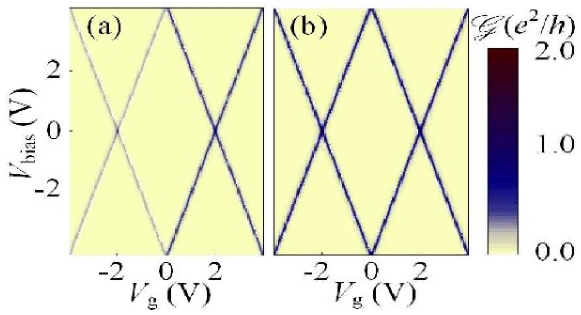
Figure 21: (Color) The stability diagram of a SSJ with $\epsilon_{\sigma}=2.0\leavevmode\nobreak\$eV, $U=4.0\leavevmode\nobreak\$eV, $\Gamma_{\textrm{L}}=\Gamma_{\textrm{R}}=0.05\leavevmode\nobreak\$eV. (a) The uncorrect result obtained by means of the widely used formula in Eq. (399) for the lesser GF is not symmetric for levels $\epsilon_{\sigma}$ and $\epsilon_{\sigma}+U$. (b) Results obtained by means of our Ansatz in Eq. (397) shows correctly symmetric for levels $\epsilon_{\sigma}$ and $\epsilon_{\sigma}+U$.

The numerical calculation results of conductance dependence on the bias and gate voltages by the two different NGF Eqs. (397) and (399) are shown in Fig. 21. As we can see in the left panel, the adoption of Eq. (399) results in an incorrectly symmetry-breaking in the gate potential. This wrong behavior is corrected in the right panel where Eq. (397) has been used.

Note, that the expressions for the retarded and lesser functions, described above, can be obtained in a more formal way by the EOM method formulated on the Keldysh contour.

(iii) Comparison with the master equation result

In the single site model with two (spin-up and spin-down) levels it is possible to make the direct comparison between our Ansatz and the master equation methods. For the latter, we used the well known master equations for quantum dots Beenakker91prb ; Averin91prb .

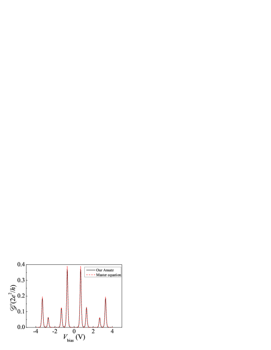
Figure 22: (Color) The comparison of the master equation method and our Ansatz for the differential conductance of the two level model with $\epsilon_{\uparrow}=-0.35\leavevmode\nobreak\$eV, $\epsilon_{\downarrow}=-0.65\leavevmode\nobreak\$eV, $U=1.0\leavevmode\nobreak\$eV, $V_{\textrm{g}}=1.0\leavevmode\nobreak\$V, $\Gamma_{\textrm{L}}=\Gamma_{\textrm{R}}=0.05\leavevmode\nobreak\$eV.

In the Fig. 22 the typical curves of the differential conductance as a function of the bias voltage at fixed gate voltage obtained by the two methods are shown together: there is basically no difference in the results obtained by these two methods. In the Fig. 23 the contour plot of the differential conductance obtained by our Ansatz is shown. We do not present here the contour plot obtained by the master equation method because it looks exactly the same.

It is quite clear from the presented figures that our Ansatz and the master equation method give essentially the same results in the limit of weak coupling to the leads. The systematic investigation of the deviations between the two methods at stronger tunneling will be presented in a separate publication.

It is important that our Ansatz can be applied straightforwardly to multilevel systems in the case when the exact eigenstates of an isolated system are unknown and the usage of the master equation method is not easy. In this paper we consider the simplest example of such a system, namely a double site case.

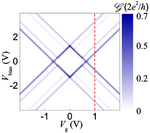
Figure 23: (Color) The stability diagram (the contour plot of the differential conductance) calculated by our Ansatz for the two level model with parameters as in Fig. 22. The latter is indicated with a dash line at $V_{\textrm{g}}=1.0\leavevmode\nobreak\$V.

Double quantum dot (two sites)

Figure 24: (Color) The general configuration of a double site junction. The levels $\epsilon_{1,2}$ with charging energies $U_{1,2}$ are connected via $t$ and coupled to the electrodes via the linewidth injection rates $\gamma^{i}_{\alpha}$.

We now return to the investigation of the DSJ system (Fig. 24) with Coulomb interaction on each site. The Hamiltonian is expressed as follows,

$$H=H_{\textrm{D}}+H_{t}+\sum_{\alpha}(H_{\alpha}+H_{\alpha\textrm{D}}),$$

where

$$\displaystyle H^{\phantom{\dagger}}_{\textrm{D}}=\sum_{i,\sigma}\epsilon^{\phantom{\dagger}}_{i,\sigma}d^{\dagger}_{i,\sigma}d^{\phantom{\dagger}}_{i,\sigma}+\frac{U_{i}}{2}n^{\phantom{\dagger}}_{i,\sigma}n^{\phantom{\dagger}}_{i,\bar{\sigma}},$$

$$\displaystyle H^{\phantom{\dagger}}_{t}=\sum_{i\neq j,\sigma}\frac{t}{2}(d^{\dagger}_{i,\sigma}d^{\phantom{\dagger}}_{j,\sigma}+d^{\dagger}_{j,\sigma}d^{\phantom{\dagger}}_{i,\sigma}),$$

$$\displaystyle H^{\phantom{\dagger}}_{\alpha,\sigma}=\sum_{k,\sigma}\epsilon^{(\alpha)}_{k,\sigma}c^{\dagger}_{\alpha,k,\sigma}c^{\phantom{\dagger}}_{\alpha,k,\sigma},$$

$$\displaystyle H^{\phantom{\dagger}}_{\alpha\textrm{D},\sigma}=\sum_{k,\sigma}\left(V^{\phantom{\dagger}}_{\alpha,k,\sigma}c^{\dagger}_{\alpha,k,\sigma}d^{\phantom{\dagger}}_{i,\sigma}+V^{*\phantom{\dagger}}_{\alpha,k,\sigma}d^{\dagger}_{i,\sigma}c^{\phantom{\dagger}}_{\alpha,k,\sigma}\right),$$

with $i,j=1,2$ indicate the site, $t$ is the constant for electron hopping between different sites.

With the help of the EOM, and by means of the truncation approximation on the double-particle GFs, we obtain the closed form for the retarded GFs as follows

$$(\omega-\epsilon^{\phantom{\dagger}}_{i,\sigma}-\Sigma^{\textrm{r}}_{i,\sigma})G^{(U,t)\textrm{r}}_{i,\sigma;j,\tau}=\delta^{\phantom{\dagger}}_{i,j}\delta^{\phantom{\dagger}}_{\sigma,\tau}+U_{i}G^{(2)(U,t)\textrm{r}}_{i,\sigma;j,\tau}+t\leavevmode\nobreak\ G^{(U,t)\textrm{r}}_{i,\sigma;j,\tau},$$ (400a)

$$(\omega-\epsilon^{\phantom{\dagger}}_{i,\sigma}-U_{i}-\Sigma^{\textrm{r}}_{i,\sigma})G^{(2)(U,t)\textrm{r}}_{i,\sigma;j,\tau}=\langle n^{\phantom{\dagger}}_{i,\bar{\sigma}}\rangle\delta^{\phantom{\dagger}}_{i,j}\delta^{\phantom{\dagger}}_{\sigma,\tau}+t\leavevmode\nobreak\ n^{\phantom{\dagger}}_{i,\bar{\sigma}}G^{(U,t)\textrm{r}}_{i,\sigma;j,\tau},$$ (400b)

where the DSJ retarded GFs are defined as

$$G^{(U,t)\textrm{r}}_{i,j;\sigma,\tau}=\langle\langle d^{\phantom{\dagger}}_{i,\sigma}|d^{\dagger}_{j,\tau}\rangle\rangle^{\textrm{r}},$$ (401)

$$G^{(2)(U,t)\textrm{r}}_{i,j;\sigma,\tau}=\langle\langle n^{\phantom{\dagger}}_{i,\bar{\sigma}}d^{\phantom{\dagger}}_{i,\sigma}|d^{\dagger}_{j,\tau}\rangle\rangle^{\textrm{r}}.$$ (402)

Here $\bar{i}$ means ‘NOT $i$’, and $\Sigma^{\textrm{r}}_{i,\sigma}$ are the electron self-energy from leads.

From Eqs. (400a), (400b) and performing the same Ansatz as in the case of SSJ, we can obtain the DSJ lesser GFs with Coulomb-interaction effects as follows

$$G^{(U,t)<}(\omega)=(1+G^{(U,t)\textrm{r}}\Sigma^{\textrm{r}}_{t})G^{(U)<}(1+\Sigma^{\textrm{a}}_{t}G^{(U,t)\textrm{a}})+G^{(U,t)\textrm{r}}\Sigma^{<}_{t}G^{(U,t)\textrm{a}},$$ (403)

with

$$\Sigma^{\textrm{r}}_{t}=\Sigma^{\textrm{a}}_{t}=\begin{pmatrix}0&t&0&0\\ t&0&0&0\\ 0&0&0&t\\ 0&0&t&0\end{pmatrix},$$

and $\Sigma^{<}_{t}=0$. $G^{(U)<}$ is the DSJ lesser GF with the same form as Eq. (397), but taking

$$U=\begin{pmatrix}U_{1}&0&0&0\\ 0&U_{2}&0&0\\ 0&0&U_{1}&0\\ 0&0&0&U_{2}\end{pmatrix},\ \Gamma_{\alpha}=\begin{pmatrix}\gamma^{1}_{\alpha}&0&0&0\\ 0&\gamma^{2}_{\alpha}&0&0\\ 0&0&\gamma^{1}_{\alpha}&0\\ 0&0&0&\gamma^{2}_{\alpha}\end{pmatrix},$$ (404)

where $\gamma^{i}_{\alpha}$ indicates the line width function of lead $\alpha$ to site $i$, and $U_{i}$ is the charging energy at site $i$. $G^{\textrm{r}/\textrm{a}}$ and $G^{(2)\textrm{r}/\textrm{a}}$ are the GF matrix from Eqs. (400a) and (400b). Here, in order to distinguish different GFs, we introduce the subscript ‘$(U,t)$’ for the one with both Coulomb interaction $U$ and inter-site hopping $t$, while ‘$(U)$’ for the one only with Coulomb interaction.

For our models, the lesser GFs in Eq. (397), (398) and (403), which are obtained with help of our Ansatz, can also be obtained by the EOM NEGF formula (331) within the same truncation approximation.

The current can be generally written as Meir92prl

$$J=\frac{\textrm{i}e}{2\hbar}\int{\frac{d\epsilon}{2\pi}}\textrm{Tr}\{(\Gamma_{\textrm{L}}-\Gamma_{\textrm{R}})G^{(U,t)<}+[f_{\textrm{L}}(\omega)\Gamma_{\textrm{L}}-f_{\textrm{R}}(\omega)\Gamma_{\textrm{R}}](G^{(U,t)\textrm{r}}-G^{(U,t)\textrm{a}})\},$$

where the lesser GF is given by Eq. (403). The differential conductance is defined as

$$\mathcal{G}=\frac{\partial J}{\partial V_{\textrm{bias}}},$$

where the bias voltage is defined as $V_{\textrm{bias}}=(\mu_{\textrm{R}}-\mu_{\textrm{L}})/e$.

(i) Serial configuration

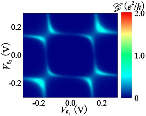
Figure 25: (Color) The stability diagram of a serial DSJ with $\epsilon_{1,\sigma}=\epsilon_{2,\sigma}=-0.15\leavevmode\nobreak\$eV, $U_{1}=U_{2}=0.3\leavevmode\nobreak\$eV, $t=0.05\leavevmode\nobreak\$eV, $\gamma^{1}_{\textrm{L}}=\gamma^{2}_{\textrm{R}}=0.02\leavevmode\nobreak\$eV, $\gamma^{2}_{\textrm{L}}=\gamma^{1}_{\textrm{R}}=0$ ,$V_{\textrm{bias}}=0.005V$. The maximums of conductance are observed when the levels of the first site ($\epsilon_{1,\sigma}$ or $\epsilon_{1,\sigma}+U$) are overlapped with the levels of the second site ($\epsilon_{2,\sigma}$ or $\epsilon_{2,\sigma}+U$), and with the Fermi energy in the leads. The splitting of the four maximums is due to the hopping between the dots.

By taking $\gamma^{2}_{L}=\gamma^{1}_{R}=0$, we obtain a serial DSJ, which could describe the kind of molecular quantum junctions like the ones studied in Ref. Elbing05pnas . First, at small bias voltages, the conductance with the two gate voltages $V_{\textrm{g}_{1}}$ and $V_{\textrm{g}_{2}}$ was calculated, and the relative stability diagram was obtained as shown in Fig. 25. Because of the double degeneracy (spin-up and spin-down) considered for each site and electrons hopping between the dots, there are eight resonance-tunnelling regions. This result is consistent with the master-equation approach. vanderWiel02rmp

Further, we studied the nonequilibrium current for large bias-voltages (Fig. 26). Because $\epsilon_{1,\sigma}$ and $\epsilon_{2,\sigma}$ are taken as asymmetric, for the case without Coulomb interaction, the $I$-$V$ curve is asymmetric for $\pm V_{\textrm{bias}}$, and there are one step and one maximum for the current. The step contributes to one peak for the conductance. When we introduce the Coulomb interaction to the system, the one conductance peak is split into several: two peaks, one pseudo-peak and one dip, while the current maximum comes to be double split (see Fig. 26). The origin of this is in the effective splitting of the degenerate level when one of the spin states is occupied and the other is empty. When both spin states are occupied, the degeneracy is restored.

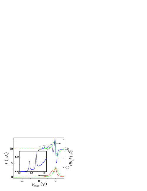
Figure 26: (Color) Current and conductance vs. bias-voltage of a DSJ far from equilibrium with parameters $\epsilon_{1,\sigma}=0.5\leavevmode\nobreak\$eV, $\epsilon_{2,\sigma}=-0.5\leavevmode\nobreak\$eV, $U_{1}=U_{2}=U=0.2\leavevmode\nobreak\$eV, $t=0.07\leavevmode\nobreak\$eV, $\gamma^{1}_{\textrm{L}}=\gamma^{2}_{\textrm{R}}=0.03\leavevmode\nobreak\$eV, $V_{\textrm{g}_{2}}=-V_{\textrm{g}_{1}}=V_{\textrm{bias}}/4$ and $V_{\textrm{R}}=-V_{\textrm{L}}=V_{\textrm{bias}}/2$. The red curve represents the current, while the blue the conductance. The inset is the blow-up for the conductance peak split. The dash and dot-dash curves are for current and conductance with $U=0$, respectively.

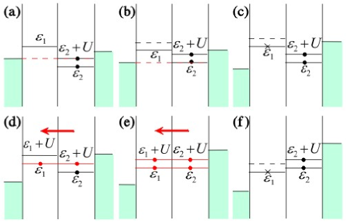
Figure 27: (Color) The processes involved in the transport characteristics in figure 26. $\epsilon_{1}\equiv\epsilon_{1,\sigma}$, $\epsilon_{2}\equiv\epsilon_{2,\sigma}$, The red line indicates electron resonant-tunnelling. a) The first conductance peak. b) The second conductance peak. c) The pseudo-peak of conductance. d) The first current maximum, and the red line indicates resonant tunnelling of electrons. e) The second current maximum for electron resonant tunnelling. f) The dip of conductance.

This process can be illustrated by the help of Fig. 27. At zero bias-voltage, $\epsilon_{2,\sigma}$ is occupied and $\epsilon_{1,\sigma}$ is empty. Then we start to increase the bias voltage. a) The level $\epsilon_{2,\sigma}+U$ is first opened for transport. It will contribute the first peak for conductance. b) Further, the levels $\epsilon_{2,\sigma}$ and $\epsilon_{1,\sigma}$ come into the transport window between the left and the right Fermi levels, resulting in the second peak. c) When the level $\epsilon_{1,\sigma}+U$ comes into play, only a pseudo-peak appears. This is because there is only a little possibility for electrons to occupy the level $\epsilon_{1,\sigma}$ under positive bias voltage. d) Levels $\epsilon_{2,\sigma}+U$ and $\epsilon_{1,\sigma}$ meet, which results in electron resonant-tunnelling and leads to the first maximum of the current. Then a new level $\epsilon_{1,\sigma}+U$ appears over the occupied $\epsilon_{1,\sigma}$ due to the Coulomb interaction. e) The meeting of $\epsilon_{2,\sigma}$ and $\epsilon_{1,\sigma}$ results in electron resonant tunnelling. It means that $\epsilon_{1,\sigma}$ will be occupied, which leads to the appearance of a new level $\epsilon_{1,\sigma}+U$. Then $\epsilon_{2,\sigma}+U$ meets $\epsilon_{1,\sigma}+U$ and another resonant tunnelling channel is opened for electrons. The two channels result in the second current maximum. f) finally, the level $\epsilon_{1,\sigma}+U$ disappears if the level $\epsilon_{1,\sigma}$ is empty. This means that a dip appears in the conductance.

It should be noted that the characteristics of serial DSJ in Fig. 26 have showed some reasonable similarities to experiments of a single-molecule diode. Elbing05pnas

(ii) Parallel configuration

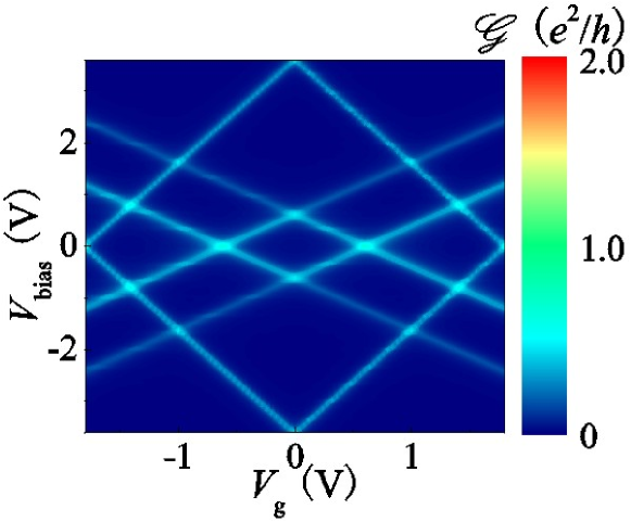
Figure 28: (Color) Nested stability diagram of a parallel DSJ with parameters $\epsilon_{1,\sigma}=-1.8\leavevmode\nobreak\$eV, $\epsilon_{2,\sigma}=-0.3\leavevmode\nobreak\$eV, $U_{1}=3.6\leavevmode\nobreak\$eV, $U_{2}=0.6\leavevmode\nobreak\$eV $t=0.001\leavevmode\nobreak\$eV, $\gamma^{1}_{\textrm{L}}=\gamma^{1}_{\textrm{R}}=0.04\leavevmode\nobreak\$eV, $\gamma^{2}_{\textrm{L}}=\gamma^{2}_{\textrm{R}}=0.05\leavevmode\nobreak\$eV, $V_{\textrm{g}_{2}}=V_{\textrm{g}_{1}}/2=V_{\textrm{g}}/2$ and $V_{\textrm{R}}=-V_{\textrm{L}}=V_{\textrm{bias}}/2$. See discussion in the text.

If on the other hand, the two sites are symmetrically connected to the electrodes, possibly with a small inter-dot hopping, but with charging energies $U_{1}$ and $U_{2}$ fixed to different scales for transport. The resulting stability diagram contains both interference effects for parallel pathways and an overlap of $U_{1}$ and $U_{2}$ stability diagrams, which we refer to a nesting characteristic. (see Fig. 28).

The physics of the weak lines in the figure can be understood by the help of charging effects. For simplicity, here we would ignore the site index $i$. In the region of large positive gate voltage at zero bias voltage, $\epsilon_{\uparrow}$ and $\epsilon_{\downarrow}$ are all empty, which means that the two levels are degenerate. Therefore adding a bias voltage, first, there will be two channels ($\epsilon_{\uparrow}$ and $\epsilon_{\downarrow}$) opened for current (thick lines). After then, one level $\epsilon_{\sigma}$ (spin-up or spin-down) is occupied, while the other obtains a shift for Coulomb interaction: $\epsilon_{\bar{\sigma}}\rightarrow\epsilon_{\bar{\sigma}}+U$. Therefore, when the bias voltage is further increased to make the Fermi-window boundary meeting level $\epsilon_{\bar{\sigma}}+U$, only one channel is opened for the current, which results in the weak lines in Fig. 28, which is the characteristic of CB. The similar case appears in the region of large negative gate voltages.

Finally, we here introduced a powerful Ansatz for the lesser Green function, which is consistent with both the Dyson-equation approach and the equation-of-motion approach. By using this Ansatz together with the standard equation-of-motion technique for the retarded and advanced Green functions, we obtained the NEGF for both the single and the double site junctions in the Coulomb blockade regime at finite voltages and calculated the transport observables. The method can be applied to describe self-consistently transport through single molecules with strong Coulomb interaction and arbitrary coupling to the leads.

To test our method, we here analyzed the CB stability diagrams for a SSJ and a DSJ. Our results are all consistent with the results of experiments and the master-equation approach. We showed, that the improved lesser Green function gives better results for weak molecule-to-contact couplings, where a comparison with the master equation approach is possible.

For the serial configuration of a DSJ, such as a donor/acceptor rectifier, the $I$-$V$ curves maintain a diode-like behavior, as it can be already inferred by coherent transport calculations. Pump07ss Besides, we predict that as a result of charging effects, one conductance peak will be split into three peaks and one dip, and one current maximum into two. For a DSJ parallel configuration, due to different charging energies on the two dot sites, the stability diagrams show peculiar nesting characteristics.

4.2 Nonequilibrium vibrons

Though the electron-vibron model described in the Section II has a long history, the many questions it implies are not answered up to now. While the isolated electron-vibron model can be solved exactly by the so-called polaron or Lang-Firsov transformation Lang63jetp ; Hewson74jjap ; Mahan90book , the coupling to the leads produces a true many-body problem. The inelastic resonant tunneling of single electrons through the localized state coupled to phonons was first considered in Refs. Glazman88jetp ; Wingreen88prl ; Wingreen89prb ; Jonson89prb . There, the exact solution in the single-particle approximation was derived, ignoring completely the Fermi sea in the leads. At strong electron-vibron couplings and weak couplings to the leads, satellites of the main resonant peak are formed in the spectral function (Fig. 11). The number of the relevant side-bands is determined by the well known Huang-Rhys factor Huang50procrsoc $g=(\lambda/\omega_{0})^{2}$. The question which remains is whether these side-bands can be observed in the differential conductance, when the coupling to all electrons in the leads should be taken into account simultaneously. New theoretical treatments were presented recently in Refs. Kral97 ; Lundin02prb ; Zhu03prb ; Braig03prb ; Flensberg03prb ; Aji03condmat ; Mitra04prb ; Frederiksen04prl ; Frederiksen04master ; Hartung04master ; Galperin04nanolett ; Galperin04jcp ; Paulsson05prb ; Galperin05nanolett ; Cizek04prb ; Cizek05czechjp ; Ryndyk05prb ; Gutierrez05nanolett ; Gutierrez05prb ; Koch05prl ; Arseyev05jetplett ; Arseyev06jetplett ; Paulsson06nanolett ; Paulsson06jpconf ; Zazunov06prb1 ; Zazunov07prb ; Koch06prb ; Koch06prb2 ; Galperin06prb ; Gutierrez06prb ; Jauho06jpcs ; Ryndyk06prb ; Frederiksen07prb ; Frederiksen07prb2 ; Galperin07jpcm ; Song07prb ; Ryndyk07prb ; Raza08prb ; Raza08condmat ; Gagliardi08njp ; DAmico08njp ; Ryndyk08preprint .

In parallel, the theory of inelastic scanning tunneling spectroscopy was developed Persson87prl ; Gata93prb ; Tikhodeev01surfsci ; Mii02surfsci ; Mii03prb ; Tikhodeev04prb ; Raza07condmat . For a recent review of the electron-vibron problem and its relation to charge transport at the molecular scale see Ref. Galperin07jpcm . Note the related problem of quantum shuttle Gorelik98prl ; Fedorets02epl ; Novotny03prl ; Fedorets04prl .

Many interesting results by the investigation of quantum transport in the strong electron-vibron coupling limit has been achieved with the help of the master equation approach Braig03prb ; Mitra04prb ; Koch05prl ; Koch06prb ; Koch06prb2 . This method, however, is valid only in the limit of very weak molecule-to-lead coupling and neglects all spectral effects, which are the most important at finite coupling to the leads.

Nonequilibrium Dyson-Keldysh method

(i) The model electron-vibron Hamiltonian

We use the minimal transport model described in the previous sections. For convenience, we present the Hamiltonian here once more. The full Hamiltonian is the sum of the molecular Hamiltonian $\hat{H}_{M}$, the Hamiltonians of the leads $\hat{H}_{R(L)}$, the tunneling Hamiltonian $\hat{H}_{T}$ describing the molecule-to-lead coupling, the vibron Hamiltonian $\hat{H}_{V}$ including electron-vibron interaction and coupling of vibrations to the environment (describing dissipation of vibrons)

$$\hat{H}=\hat{H}_{M}+\hat{H}_{V}+\hat{H}_{L}+\hat{H}_{R}+\hat{H}_{T}.$$ (405)

A molecule is described by a set of localized states $|\alpha\rangle$ with energies $\epsilon_{\alpha}$ and inter-orbital overlap integrals $t_{\alpha\beta}$ by the following model Hamiltonian:

$$\hat{H}^{(0)}_{M}=\sum_{\alpha}\left(\epsilon_{\alpha}+e\varphi_{\alpha}(t)\right)d^{{\dagger}}_{\alpha}d^{\phantom{{\dagger}}}_{\alpha}+\sum_{\alpha\neq\beta}t_{\alpha\beta}d^{{\dagger}}_{\alpha}d^{\phantom{{\dagger}}}_{\beta}.$$ (406)

Vibrations and the electron-vibron coupling are described by the Hamiltonian Frederiksen04prl ; Frederiksen04master ; Hartung04master ; Ryndyk06prb ($\hbar=1$)

$$\hat{H}_{V}=\sum_{q}\omega_{q}a_{q}^{\dagger}a^{\phantom{{\dagger}}}_{q}+\sum_{\alpha\beta}\sum_{q}\lambda^{q}_{\alpha\beta}(a^{\phantom{{\dagger}}}_{q}+a_{q}^{\dagger})d^{{\dagger}}_{\alpha}d^{\phantom{{\dagger}}}_{\beta}.$$ (407)

Here vibrations are considered as localized phonons and $q$ is an index labeling them, not the wave-vector. The first term describes free vibrons with the energy $\omega_{q}$. The second term represents the electron-vibron interaction. We include both diagonal coupling, which describes a change of the electrostatic energy with the distance between atoms, and the off-diagonal coupling, which describes the dependence of the matrix elements $t_{\alpha\beta}$ over the distance between atoms.

The Hamiltonians of the right (R) and left (L) leads read

$$\hat{H}_{i=L(R)}=\sum_{k\sigma}(\epsilon_{ik\sigma}+e\varphi_{i})c^{{\dagger}}_{ik\sigma}c^{\phantom{{\dagger}}}_{ik\sigma},$$ (408)

$\varphi_{i}(t)$ are the electrical potentials of the leads. Finally, the tunneling Hamiltonian

$$\hat{H}_{T}=\sum_{i=L,R}\sum_{k\sigma,\alpha}\left(V_{ik\sigma,\alpha}c^{{\dagger}}_{ik\sigma}d_{\alpha}+{\rm h.c.}\right)$$ (409)

describes the hopping between the leads and the molecule. A direct hopping between two leads is neglected.

(ii) Keldysh-Dyson equations and self-energies

We use the nonequilibrium Green function (NGF) method, as introduced in Section III. The current in the left ($i=L$) or right ($i=R$) contact to the molecule is described by the expression

$$J_{i=L,R}=\frac{ie}{\hbar}\int\frac{d\epsilon}{2\pi}{\rm Tr}\left\{{\bf\Gamma}_{i}(\epsilon-e\varphi_{i})\left({\bf G}^{<}(\epsilon)+f^{0}_{i}(\epsilon-e\varphi_{i})\left[{\bf G}^{R}(\epsilon)-{\bf G}^{A}(\epsilon)\right]\right)\right\},$$ (410)

where $f^{0}_{i}(\epsilon)$ is the equilibrium Fermi distribution function with chemical potential $\mu_{i}$, and the level-width function is

$${\bf\Gamma}_{i=L(R)}(\epsilon)=\Gamma_{i\alpha\beta}(\epsilon)=2\pi\sum_{k\sigma}V_{ik\sigma,\beta}V^{*}_{ik\sigma,\alpha}\delta(\epsilon-\epsilon_{ik\sigma}).$$

The lesser (retarded, advanced) Green function matrix of a nonequilibrium molecule ${\bf G}^{<(R,A)}\equiv G_{\alpha\beta}^{<(R,A)}$ can be found from the Dyson-Keldysh equations in the integral form

$${\bf G}^{R}(\epsilon)={\bf G}^{R}_{0}(\epsilon)+{\bf G}^{R}_{0}(\epsilon){\bf\Sigma}^{R}(\epsilon){\bf G}^{R}(\epsilon),$$ (411)

$${\bf G}^{<}(\epsilon)={\bf G}^{R}(\epsilon){\bf\Sigma}^{<}(\epsilon){\bf G}^{A}(\epsilon),$$ (412)

or from the corresponding equations in the differential form (see e.g. Refs. Ryndyk05prb ; Ryndyk06prb and references therein).

Here

$${\bf\Sigma}^{R,<}={\bf\Sigma}^{R,<(T)}_{L}+{\bf\Sigma}^{R,<(T)}_{R}+{\bf\Sigma}^{R,<(V)}$$ (413)

is the total self-energy of the molecule composed of the tunneling (coupling to the left and right leads) self-energies

$${\bf\Sigma}_{j=L,R}^{R,<(T)}\equiv{\Sigma}_{j\alpha\beta}^{R,<(T)}=\sum_{k\sigma}\left\{V^{*}_{jk\sigma,\alpha}{G}^{R,<}_{jk\sigma}V_{jk\sigma,\beta}\right\},$$ (414)

and the vibronic self-energy ${{\bf\Sigma}}^{R,<(V)}\equiv{\Sigma}^{R,<(V)}_{\alpha\beta}$.

For the retarded tunneling self-energy ${\bf\Sigma}_{i}^{R(T)}$ one obtains

$${\bf\Sigma}^{R(T)}_{i}(\epsilon)={\bf\Lambda}_{i}(\epsilon-e\varphi_{i})-\frac{\mathrm{i}}{2}{\bf\Gamma}_{i}(\epsilon-e\varphi_{i}),$$ (415)

where ${\bf\Lambda}_{i}$ is the real part of the self-energy, which usually can be included in the single-particle Hamiltonian $\hat{H}^{(0)}_{M}$, and ${\bf\Gamma}_{i}$ describes level broadening due to coupling to the leads. For the corresponding lesser function one finds

$${\bf\Sigma}^{<(T)}_{i}(\epsilon)=\mathrm{i}{\bf\Gamma}_{i}(\epsilon-e\varphi_{i})f^{0}_{i}(\epsilon-e\varphi_{i}).$$ (416)

In the standard self-consistent Born approximation, using the Keldysh technique, one obtains for the vibronic self-energies Mitra04prb ; Frederiksen04prl ; Frederiksen04master ; Hartung04master ; Galperin04nanolett ; Galperin04jcp ; Galperin07jpcm ; Ryndyk06prb

$$\displaystyle{\bf\Sigma}^{R(V)}(\epsilon)=\frac{i}{2}\sum_{q}\int\frac{d\omega}{2\pi}\left({\bf M}^{q}{\bf G}^{R}_{\epsilon-\omega}{\bf M}^{q}D^{K}_{q\omega}+\right.$$

$$\displaystyle\left.+{\bf M}^{q}{\bf G}^{K}_{\epsilon-\omega}{\bf M}^{q}D^{R}_{q\omega}-2D^{R}_{q\omega=0}{\bf M}^{q}{\rm Tr}\left[{\bf G}^{<}_{\omega}{\bf M}^{q}\right]\right),$$ (417)

$$\displaystyle{\bf\Sigma}^{<(V)}(\epsilon)=i\sum_{q}\int\frac{d\omega}{2\pi}{\bf M}^{q}{\bf G}^{<}_{\epsilon-\omega}{\bf M}^{q}D^{<}_{q\omega},$$ (418)

where ${\bf G}^{K}=2{\bf G}^{<}+{\bf G}^{R}-{\bf G}^{A}$ is the Keldysh Green function, and ${\bf M}^{q}\equiv M^{q}_{\alpha\beta}$.

If vibrons are noninteracting, in equilibrium, and non-dissipative, then the vibronic Green functions write:

$$D^{R}_{0}(q,\omega)=\frac{1}{\omega-\omega_{q}+\mathrm{i}0^{+}}-\frac{1}{\omega+\omega_{q}+\mathrm{i}0^{+}},$$ (419)

$$D^{<}_{0}(q,\omega)= -2\pi\mathrm{i}\left[(f_{B}^{0}(\omega_{q})+1)\delta(\omega+\omega_{q})+f_{B}^{0}(\omega_{q})\delta(\omega-\omega_{q})\right],$$ (420)

where the equilibrium Bose distribution function is

$$f_{B}^{0}(\omega)=\frac{1}{\exp\left(\omega/T\right)-1}.$$ (421)

In the Migdal model the retarded vibron function is calculated from the Dyson-Keldysh equation

$$D^{R}(q,\omega)=\frac{2\omega_{q}}{\omega^{2}-\omega^{2}_{q}-2\omega_{q}{\Pi}^{R}(q,\omega)},$$ (422)

where $\Pi(q,\omega)$ is the polarization operator (boson self-energy). The equation for the lesser function (quantum kinetic equation in the integral form) is

$$(\Pi^{R}_{q\omega}-\Pi^{A}_{q\omega})D^{<}_{q\omega}-(D^{R}_{q\omega}-D^{A}_{q\omega})\Pi^{<}_{q\omega}=0,$$ (423)

this equation in the stationary case considered here is algebraic in the frequency domain.

The polarization operator is the sum of two parts, environmental and electronic: $\Pi^{R,<}_{q\omega}=\Pi^{R,<(\rm env)}_{q\omega}+\Pi^{R,<(\rm el)}_{q\omega}$.

The environmental equilibrium part of the polarization operator can be approximated by the simple expressions

$$\displaystyle\Pi^{R(\rm env)}(q,\omega)=-\frac{i}{2}\gamma_{q}{\rm sign}(\omega),$$ (424)

$$\displaystyle\Pi^{<(\rm env)}(q,\omega)=-i\gamma_{q}f_{B}^{0}(\omega){\rm sign}(\omega),$$ (425)

where $\gamma_{g}$ is the vibronic dissipation rate, and $f_{B}^{0}(\omega)$ is the equilibrium Bose-Einstein distribution function.

The electronic contribution to the polarization operator within the SCBA is

$$\Pi^{R(\rm el)}(q,\omega)=-i\int\frac{d\epsilon}{2\pi}{\rm Tr} \left({\bf M}^{q}{\bf G}^{<}_{\epsilon}{\bf M}^{q}{\bf G}^{A}_{\epsilon-\omega}+{\bf M}^{q}{\bf G}^{R}_{\epsilon}{\bf M}^{q}{\bf G}^{<}_{\epsilon-\omega}\right),$$ (426)

$$\Pi^{<(\rm el)}(q,\omega)=-i\int\frac{d\epsilon}{2\pi}{\rm Tr} \left({\bf M}^{q}{\bf G}^{<}_{\epsilon}{\bf M}^{q}{\bf G}^{>}_{\epsilon-\omega}\right).$$ (427)

We obtained the full set of equations, which can be used for numerical calculations.

Single-level model: spectroscopy of vibrons

The isolated single-level electron-vibron model is described by the Hamiltonian

$$\hat{H}_{M+V}=(\epsilon_{0}+e\varphi_{0})d^{{\dagger}}d+\omega_{0}a^{{\dagger}}a+\lambda\left(a^{{\dagger}}+a\right)d^{{\dagger}}d,$$ (428)

where the first and the second terms describe the free electron state and the free vibron, and the third term is electron-vibron minimal coupling interaction.

The electrical potential of the molecule $\varphi_{0}$ plays an important role in transport at finite voltages. It describes the shift of the molecular level by the bias voltage, which is divided between the left lead (tip), the right lead (substrate), and the molecule as $\varphi_{0}=\varphi_{R}+\eta(\varphi_{L}-\varphi_{R})$ Datta97prl . We assume the simplest linear dependence of the molecular potential ($\eta=const$), but its nonlinear dependence Rakshit05 can be easily included in our model.

Here we assume, that the vibrons are in equilibrium and are not excited by the current, so that the self-consistent Born approximation is a good starting point. The vibron Green function are assumed to be equilibrium with the broadening defined by the external thermal bath, see for details Refs. Frederiksen04master ; Galperin04nanolett ; Galperin04jcp ; Galperin07jpcm ; Ryndyk06prb .

Figure 29: (Color online) Spectral function at different electron-vibron couplings: $\lambda/\omega_{0}=0.4$ (black), $\lambda/\omega_{0}=1.2$ (blue, dashed), and $\lambda/\omega_{0}=2$ (red); at $\epsilon_{0}/\omega_{0}=5$, $\Gamma_{L}/\omega_{0}=\Gamma_{R}/\omega_{0}=0.1$. In the insert the spectral function at $\lambda/\omega_{0}=1.2$ is shown at finite voltage, when the level is partially filled. Energies are in units of $\hbar\omega_{0}$.

For the single-level model all equations are significantly simplified. Combining $J_{L}$ and $J_{R}$ the expression for the current can be written for energy independent $\Gamma_{L(R)}$ (wide-band limit) as

$$J=\frac{e}{h}\frac{\Gamma_{L}\Gamma_{R}}{\Gamma_{R}+\Gamma_{L}}\int d\epsilon A(\epsilon)\left[f^{0}(\epsilon-e\varphi_{L})-f^{0}(\epsilon-e\varphi_{R})\right].$$ (429)

It looks as simple as the Landauer-Büttiker formula, but it is not trivial, because the spectral density $A(\epsilon)=-2{\rm Im}G^{R}(\epsilon)$ now depends on the distribution function of the electrons in the fluctuating molecule and hence the applied voltage, $\varphi_{L}=-\varphi_{R}=V/2$ Ryndyk05prb . Indeed, $G^{R}(\epsilon)$ can be found from (201)

$$G^{R}(\epsilon)=\frac{1}{\epsilon-\tilde{\epsilon}_{0}-\Sigma^{R(V)}(\epsilon)+i(\Gamma_{L}+\Gamma_{R})/2},$$ (430)

where $\Sigma^{R(V)}(\epsilon)$ is a functional of the electron distribution function inside a molecule. Actually, the lesser function $G^{<}(\epsilon)$ is used in the quantum kinetic formalism as a distribution function. In the single-level case the usual distribution function can be introduced through the relation

$$G^{<}(\epsilon)=iA(\epsilon)f(\epsilon).$$ (431)

Figure 30: Differential conductance of a symmetric junction ($\eta=0.5$, $\Gamma_{R}=\Gamma_{L}$) at different molecule-to-lead coupling, from $\Gamma_{L}/\omega_{0}=0.1$ (lower curve) to $\Gamma_{L}/\omega_{0}=10$ (upper curve), $\lambda/\omega_{0}=1$, $\epsilon_{0}/\omega_{0}=2$. Voltage is in the units of $\hbar\omega_{0}/e$.

Note the essential difference between symmetric ($\Gamma_{L}=\Gamma_{R}$) and asymmetric junctions. It is clear from the noninteracting solution of the transport problem. Neglecting for a moment the vibron self-energies, we obtain the noninteracting distribution function

$$f(\epsilon)=\frac{\Gamma_{L}f_{L}^{0}(\epsilon-e\varphi_{L})+\Gamma_{R}f_{R}^{0}(\epsilon-e\varphi_{R})}{\Gamma_{L}+\Gamma_{R}}.$$ (432)

For strongly asymmetric junctions (e.g. $\Gamma_{L}\ll\Gamma_{R}$) the distribution function remains close to the equilibrium function in the right lead $f_{R}^{0}(\epsilon-e\varphi_{R})$, thus essentially simplifying the solution. While for symmetric junctions the distribution function has the double-step form and is very different from the equilibrium one.

A typical example of the spectral function at zero voltage is shown in Fig. 29. At finite voltage it should be calculated self-consistently. In the insert the spectral function of the symmetric junction at finite voltage is shown, it is changed essentially because the distribution function is changed.

Let us discuss a general picture of the vibronic transport in symmetric and asymmetric single-molecule junctions, provided in experiments with the molecular bridges and STM-to-molecule junctions, respectively. The differential conductance, calculated at different molecule-to-lead coupling, is shown in Fig. 30 (symmetric) and Fig. 31 (asymmetric). At weak coupling, the vibronic side-band peaks are observed, reproducing the corresponding peaks in the spectral function. At strong couplings the broadening of the electronic state hides the side-bands, and new features become visible. In the symmetric junction, a suppression of the conductance at $V\simeq\pm\hbar\omega_{0}$ takes place as a result of inelastic scattering of the coherently transformed from the left lead to the right lead electrons. In the asymmetric junction (Fig. 31), the usual IETS increasing of the conductance is observed at a negative voltage $V\simeq-\hbar\omega_{0}$, this feature is weak and can be observed only in the incoherent tail of the resonant conductance. We conclude, that the vibronic contribution to the conductance can be distinguished clearly in both coherent and tunneling limits.

Figure 31: Differential conductance of an asymmetric junction ($\eta=0$, $\Gamma_{R}=20\Gamma_{L}$) at different molecule-to-lead coupling, from $\Gamma_{R}/\omega_{0}=0.2$ (lower curve) to $\Gamma_{R}/\omega_{0}=4$ (upper curve), $\lambda/\omega_{0}=2$, $\epsilon_{0}/\omega_{0}=5$. The voltage is in the units of $\hbar\omega_{0}/e$

Now let us discuss the particular situation of STS experiments Qiu04prl ; Wu04prl ; Repp05prl ; Repp05prl2 . Here we concentrate mainly on the dependence on the tip-to-molecule distance Wu04prl . When the tip (left lead in our notations) is far from the molecule, the junction is strongly asymmetric: $\Gamma_{L}\ll\Gamma_{R}$ and $\eta\rightarrow 0$, and the conductance is similar to that shown in Fig. 31. When the tip is close to the molecule, the junction is approximately symmetric: $\Gamma_{L}\approx\Gamma_{R}$ and $\eta\approx 0.5$, and the conductance curve is of the type shown in Fig. 30. We calculated the transformation of the conductance from the asymmetric to symmetric case (Fig. 32). It is one new feature appeared in asymmetric case due to the fact that we started from a finite parameter $\eta=0.2$ (in the Fig. 31 $\eta=0$), namely a single peak at negative voltages, which is shifted to smaller voltage in the symmetric junction. The form and behavior of this peak is in agreement with experimental results Wu04prl .

Figure 32: (Color) Differential conductance at different molecule-to-STM coupling (see the text), from asymmetric junction with $\Gamma_{L}/\omega_{0}=0.025$, $\Gamma_{R}/\omega_{0}=0.5$ and $\eta=0.2$ (lower curve, blue thick line) to symmetric junction with $\Gamma_{L}/\omega_{0}=\Gamma_{R}/\omega_{0}=0.5$ and $\eta=0.5$ (upper curve, red thick line), $\lambda/\omega_{0}=1$, $\epsilon_{0}/\omega_{0}=2$. Voltage is in the units of $\hbar\omega_{0}/e$

In conclusion, at weak molecule-to-lead (tip, substrate) coupling the usual vibronic side-band peaks in the differential conductance are observed; at stronger coupling to the leads (broadening) these peaks are transformed into step-like features. A vibronic-induced decreasing of the conductance with voltage is observed in high-conductance junctions. The usual IETS feature (increasing of the conductance) can be observed only in the case of low off-resonant conductance. By changing independently the bias voltage and the tip position, it is possible to determine the energy of molecular orbitals and the spectrum of molecular vibrations. In the multi-level systems with strong electron-electron interaction further effects, such as Coulomb blockade and Kondo effect, could dominate over the physics which we address here; these effects have to be included in a subsequent step.

Multi-level model: nonequilibrium vibrons

Basically there are two main nonequilibrium effects: the electronic spectrum modification and excitation of vibrons (quantum vibrations). In the weak electron-vibron coupling case the spectrum modification is usually small (which is dependent, however, on the vibron dissipation rate, temperature, etc.) and the main possible nonequilibrium effect is the excitation of vibrons at finite voltages. We have developed an analytical theory for this case Ryndyk06prb . This theory is based on the self-consistent Born approximation (SCBA), which allows to take easily into account and calculate nonequilibrium distribution functions of electrons and vibrons.

If the mechanical degrees of freedom are coupled strongly to the environment (dissipative vibron), then the dissipation of molecular vibrations is determined by the environment. However, if the coupling of vibrations to the leads is weak, we should consider the case when the vibrations are excited by the current flowing through a molecule, and the dissipation of vibrations is also determined essentially by the coupling to the electrons. Here , we show that the effects of vibron emission and vibronic instability are important especially in the case of electron-vibron resonance.

We simplify the equations and obtain some analytical results in the vibronic quasiparticle approximation, which assumes weak electron-vibron coupling limit and weak external dissipation of vibrons:

$$\gamma^{*}_{q}=\gamma_{q}-2{\rm Im}\Pi^{R}(\omega_{q})\ll\omega_{q}.$$ (433)

So that the spectral function of vibrons can be approximated by the Dirac $\delta$, and the lesser function reads

$$D^{<}(q,\omega)=-2\pi i\left[(N_{q}+1)\delta(\omega+\omega_{q})+N_{q}\delta(\omega-\omega_{q})\right],$$ (434)

where $N_{q}$ is (nonequilibrium) number of vibrations in the $q$-th mode. So, in this approximation the spectrum modification of vibrons is not taken into account, but the possible excitation of vibrations is described by the nonequilibrium $N_{q}$. The dissipation of vibrons is neglected in the spectral function, but is taken into account later in the kinetic equation for $N_{q}$. A similar approach to the single-level problem was considered recently in Tikhodeev01surfsci ; Mii02surfsci ; Mii03prb ; Tikhodeev04prb ; Mitra04prb ; Galperin04nanolett ; Galperin04jcp . The more general case with broadened equilibrium vibron spectral function seems to be not very interesting, because in this case vibrons are not excited. Nevertheless, in the numerical calculation it can be easy taken into consideration.

From the general quantum kinetic equation for vibrons, we obtain in this limit

$$N_{q}=\frac{\gamma_{q}N^{0}_{q}-{\rm Im}\Pi^{<}(\omega_{q})}{\gamma_{q}-2{\rm Im}\Pi^{R}(\omega_{q})}.$$ (435)

This expression describes the number of vibrons $N_{q}$ in a nonequilibrium state, $N^{0}_{q}=f_{B}^{0}(\omega_{q})$ is the equilibrium number of vibrons. In the linear approximation the polarization operator is independent of $N_{q}$ and $-2{\rm Im}\Pi^{R}(\omega_{q})$ describes additional dissipation. Note that in equilibrium $N_{q}\equiv N^{0}_{q}$ because ${\rm Im}\Pi^{<}(\omega_{q})=2{\rm Im}\Pi^{R}(\omega_{q})f_{B}^{0}(\omega_{q})$. See also detailed discussion of vibron emission and absorption rates in Refs. Tikhodeev01surfsci ; Mii02surfsci ; Mii03prb ; Tikhodeev04prb .

For weak electron-vibron coupling the number of vibrons is close to equilibrium and is changed because of vibron emission by nonequilibrium electrons, $N_{q}$ is roughly proportional to the number of such electrons, and the distribution function of nonequilibrium electrons is not change essentially by the interaction with vibrons (perturbation theory can be used). The situation changes, however, if nonequilibrium dissipation $-2{\rm Im}\Pi^{R}(\omega_{q})$ is negative. In this case the number of vibrons can be essentially larger than in the equilibrium case (vibronic instability), and the change of electron distribution function should be taken into account self-consistently.

In the stationary state the nonlinear dissipation rate

$$\gamma^{*}_{q}=\gamma_{q}-2{\rm Im}\Pi^{R}(\omega_{q})$$ (436)

is positive, but the nonequilibrium contribution to dissipation $-2{\rm Im}\Pi^{R}(\omega_{q})$ remains negative.

Additionally to the vibronic quasiparticle approximation, the electronic quasiparticle approximation can be used when the coupling to the leads is weak. In this case the lesser function can be parameterized through the number of electrons $F_{\eta}$ in the eigenstates of the noninteracting molecular Hamiltonian $H^{(0)}_{M}$

$$G^{<}_{\alpha\beta}=i\sum_{\gamma\eta}A_{\alpha\gamma}S_{\gamma\eta}F_{\eta}S^{-1}_{\eta\beta},$$ (437)

we introduce the unitary matrix $\bf S$, which transfer the Hamiltonian ${\bf H}\equiv H^{(0)}_{M\alpha\beta}$ into the diagonal form ${\bf\tilde{H}}={\bf S}^{-1}{\bf H}{\bf S}$, so that the spectral function of this diagonal Hamiltonian is

$$\tilde{A}_{\delta\eta}(\epsilon)=2\pi\delta(\epsilon-\tilde{\epsilon}_{\delta})\delta_{\delta\eta},$$ (438)

where $\tilde{\epsilon}_{\delta}$ are the eigenenergies.

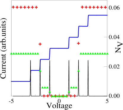
Figure 33: (Color) Vibronic emission in the symmetric multilevel model: voltage-current curve, differential conductance, and the number of excited vibrons in the off-resonant (triangles) and resonant (crosses) cases (details see in the text).

Note that in the calculation of the self-energies and polarization operators we can not use $\delta$-approximation for the spectral function (this is too rough and results in the absence of interaction out of the exact electron-vibron resonance). So that in the calculation we use actually (437) with broadened equilibrium spectral function. This approximation can be systematically improved by including nonequilibrium corrections to the spectral function, which are important near the resonance. It is important to comment that for stronger electron-vibron coupling vibronic side-bands are observed in the spectral function and voltage-current curves at energies $\tilde{\epsilon}_{\delta}\pm n\omega_{q}$, we do not consider these effects in the rest of our paper and concentrate on resonance effects.

After correspondingly calculations we obtain finally

$$N_{q}=\frac{\gamma_{q}N^{0}_{q}-\sum_{\eta\delta}\kappa_{\eta\delta}(\omega_{q})F_{\eta}(F_{\delta}-1)}{\gamma_{q}-\sum_{\eta\delta}\kappa_{\eta\delta}(\omega_{q})(F_{\eta}-F_{\delta})},$$ (439)

where coefficients $\kappa_{\eta\delta}$ are determined by the spectral function and electron-vibron coupling in the diagonal representation

$$\kappa_{\eta\delta}(\omega_{q})=\int\frac{d\epsilon}{2\pi}\tilde{M}^{q}_{\eta\delta}\tilde{A}_{\delta\delta}(\epsilon-\omega_{q})\tilde{M}^{q}_{\delta\eta}\tilde{A}_{\eta\eta}(\epsilon),$$ (440)

$$F_{\eta}=\frac{\tilde{\Gamma}_{L\eta\eta}f^{0}_{L\eta}\!+\!\tilde{\Gamma}_{R\eta\eta}f^{0}_{R\eta}\!+\!\sum_{q\eta}\left[\zeta^{-q}_{\eta\delta}F_{\delta}N_{q}\!+\!\zeta^{+q}_{\eta\delta}F_{\delta}(1\!+\!N_{q})\right]}{\tilde{\Gamma}_{L\eta\eta}\!+\!\tilde{\Gamma}_{R\eta\eta}\!+\!\sum_{q\eta}\left[\zeta^{-q}_{\eta\delta}(1\!-\!F_{\delta}\!+\!N_{q})\!+\!\zeta^{+q}_{\eta\delta}(F_{\delta}\!+\!N_{q})\right]},$$ (441)

$$\zeta^{\pm q}_{\eta\delta}=\tilde{M}^{q}_{\eta\delta}\tilde{A}_{\delta\delta}(\tilde{\epsilon}_{\eta}\pm\omega_{q})\tilde{M}^{q}_{\delta\eta},$$ (442)

here $\tilde{\Gamma}_{i\eta\eta}$ and $f^{0}_{i\eta}$ are the level width matrix in the diagonal representation and Fermi function at energy $\tilde{\epsilon}_{\eta}-e\varphi_{i}$.

These kinetic equations are similar to the usual golden rule equations, but are more general.

Now let us consider several examples of vibron emission and vibronic instability.

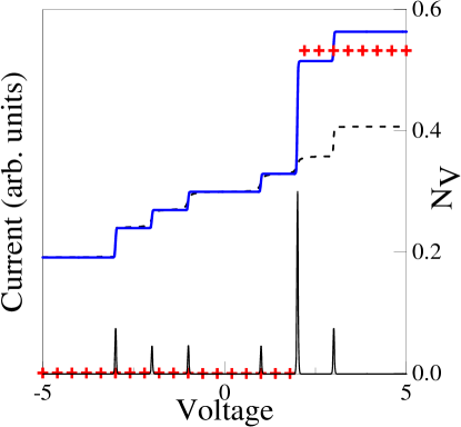
Figure 34: (Color) Vibronic instability in an asymmetric multilevel model: voltage-current curve, differential conductance, and the number of excited vibrons (crosses). Dashed line show the voltage-current curve without vibrons (details see in the text).

First we consider the most simple case, when the instability is not possible and only vibron emission takes place. This corresponds to a negative imaginary part of the electronic polarization operator: ${\rm Im}\Pi^{R)}(\omega_{q})<0$. From the Eq. (440) one can see that for any two levels with the energies $\tilde{\epsilon}_{\eta}>\tilde{\epsilon}_{\delta}$ the coefficient $\kappa_{\eta\delta}$ is larger than $\kappa_{\delta\eta}$, because the spectral function $\tilde{A}_{\delta\delta}(\epsilon)$ has a maximum at $\epsilon=\tilde{\epsilon}_{\delta}$. The contribution of $\kappa_{\eta\delta}(\omega_{q})(F_{\eta}-F_{\delta})$ is negative if $F_{\eta}<F_{\delta}$. This takes place in equilibrium, and in nonequilibrium for transport through symmetric molecules, when higher energy levels are populated after lower levels. The example of such a system is shown in Fig. 33. Here we consider a simple three-level system ($\tilde{\epsilon}_{1}=1$, $\tilde{\epsilon}_{2}=2$, $\tilde{\epsilon}_{3}=3$) coupled symmetrically to the leads ($\Gamma_{L\eta}=\Gamma_{R\eta}=0.01$). The current-voltage curve is the same with and without vibrations in the case of symmetrical coupling to the leads and in the weak electron-vibron coupling limit (if we neglect change of the spectral function). The figure shows how vibrons are excited, the number of vibrons $N_{V}$ in the mode with frequency $\omega_{0}$ is presented in two cases. In the off-resonant case (green triangles) $N_{V}$ is very small comparing with the resonant case ($\omega_{0}=\tilde{\epsilon}_{2}-\tilde{\epsilon}_{1}$, red crosses, the vertical scale is changed for the off-resonant points). In fact, if the number of vibrons is very large, the spectral function and voltage-current curve are changed. We shall consider this in a separate publication.

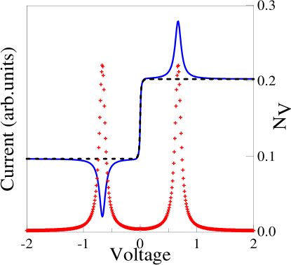
Figure 35: (Color) Floating level resonance: voltage-current curve and the number of excited vibrons (crosses). Dashed line show the voltage-current curve without vibrons (details see in the text).

Now let us consider the situation when the imaginary part of the electronic polarization operator can be positive: ${\rm Im}\Pi^{R}(\omega_{q})>0$. Above we considered the normal case when the population of higher energy levels is smaller than lower levels. The opposite case $F_{2}>F_{1}$ is known as inversion in laser physics. Such a state is unstable if the total dissipation $\gamma^{*}_{q}$ (436) is negative, which is possible only in the nonstationary case. As a result of the instability, a large number of vibrons is excited, and in the stationary state $\gamma^{*}_{q}$ is positive. This effect can be observed for transport through asymmetric molecules, when higher energy levels are populated before lower levels. The example of a such system is shown in Fig. 34. It is the same three-level system as before, but the first and second levels are coupled not symmetrically to the leads ($\Gamma_{L1}=0.001$, $\Gamma_{R1}=0.1$, $\Gamma_{L2}=0.1$, $\Gamma_{R2}=0.001$). The vibron couple resonantly these levels ($\omega_{q}=\tilde{\epsilon}_{2}-\tilde{\epsilon}_{1}$). The result is qualitatively different from the symmetrical case. The voltage-current curve is now asymmetric, a large step corresponds to the resonant level with inverted population.

Note the importance of the off-diagonal electron-vibron coupling for the resonant effects. If the matrix $\bf\tilde{M}$ in the eigen-state representation is diagonal, there is no resonant coupling between different electronic states.

Finally, let us consider the important case, when initially symmetric molecule becomes asymmetric when the external voltage is applied. The reason for such asymmetry is simply that in the external electric field left and right atoms feel different electrical potentials and the position of the levels $\epsilon_{\alpha}=\epsilon^{(0)}_{\alpha}+e\varphi_{\alpha}$ is changed (float) with the external voltage. The example of a such system is shown in Fig. 35. Here we consider a two-level system, one level is coupled electrostatically to the left lead $\tilde{\epsilon}_{1}\propto\varphi_{L}$, the other level to the right lead $\tilde{\epsilon}_{2}\propto\varphi_{R}$, the tunneling coupling to the leads also is not symmetrical ($\Gamma_{L1}=0.1$, $\Gamma_{R1}=0.001$, $\Gamma_{L2}=0.001$, $\Gamma_{R2}=0.1$). The frequency of the vibration, coupling these two states, is $\omega_{0}=1$. When we sweep the voltage, a peak in the voltage-current curve is observed when the energy difference $\tilde{\epsilon}_{1}-\tilde{\epsilon}_{2}\propto eV$ is going through the resonance $\tilde{\epsilon}_{1}-\tilde{\epsilon}_{2}\approx\omega_{0}$.

4.3 Coupling to a vibrational contiuum: dissipation and renormalization

The model Hamiltonian

In the previous section we have dealt with a simple, but nevertheless physically rich, model describing the interaction of an electronic level with some specific vibrational mode confined to the quantum dot. We have seen how to apply in this case the Keldysh non-equilibrium techniques described in Section III within the self-consistent Born and Migdal approximations. The latter are however appropriate for the weak coupling limit to the vibrational degrees of freedom. In the opposite case of strong coupling, different techniques must be applied. For equilibrium problems, unitary transformations combined with variational approaches can be used, in non-equilibrium only recently some attempts were made to deal with the problem. Galperin06prb

In this section we will consider the case of a multi-level electronic system in interaction with a bosonic bath Gutierrez05nanolett ; Gutierrez05prb . We will use unitary transformation techniques to deal with the problem, but will only focus on the low-bias transport, so that strong non-equilibrium effects can be disregarded. Our interest is to explore how the qualitative low-energy properties of the electronic system are modified by the interaction with the bosonic bath. We will see that the existence of a continuum of vibrational excitations (up to some cut-off frequency) dramatically changes the analytic properties of the electronic Green function and may lead in some limiting cases to a qualitative modification of the low-energy electronic spectrum. As a result, the $I$-$V$ characteristics at low bias may display “metallic” behavior (finite current) even if the isolated electronic system does exhibit a band gap. The model to be discussed below has been motivated by the very exciting electrical transport measurements on short poly(dG)-poly(dC) DNA molecular wires carried out at the group of N. Tao some time ago Xu04nanolett . Peculiar in these experiments was the large measured currents -up to 150 nA at 0.8 V- at low voltages, which stood in strong contrast to the usually accepted view that DNA should behave as an insulator at low applied bias. Further, a power-law length scaling of the linear conductance with increasing wire length was demonstrated, indicating that long-range charge transport was possible. Since the experiments were carried out in an aqueous solution, the possibility of a solvent-induced modification of the low-energy transport properties of the wire lied at hand, although additional factors like internal vibrations could also play a role.

The proposed model is based on an earlier work Cuniberti02prb and assumes, within a minimal tight-binding picture, that the DNA electronic states can be qualitatively classified into extended (conducting) and localized (non-conducting) states. The former may correspond e.g. to the $\pi$-orbital stack of the base pairs, the latter to energetically deeper lying (w.r.t. the frontier orbitals) base-pair states or sugar-phosphate backbone states. A further assumption is that any modification of the conducting states through the environment only takes place through a coupling to the non-conducting set. The tight-binding electronic Hamiltonian for $N$ sites can then be written as (see also Fig. 36):

$${\cal H}_{\textrm{el}} = \epsilon_{b}\sum_{j}b^{\dagger}_{j}b_{j}-t_{||}\sum_{j}\left[b^{\dagger}_{j}b_{j+1}+\textrm{H.c.}\right]+\epsilon\sum_{j}c^{\dagger}_{j}c_{j}$$ (443)

$$- t_{\perp}\sum_{j}\left[b^{\dagger}_{j}c_{j}+\textrm{H.c.}\right]={\cal H}_{\textrm{C}}+{\cal H}_{\textrm{b}}+{\cal H}_{\textrm{C-b}}.$$

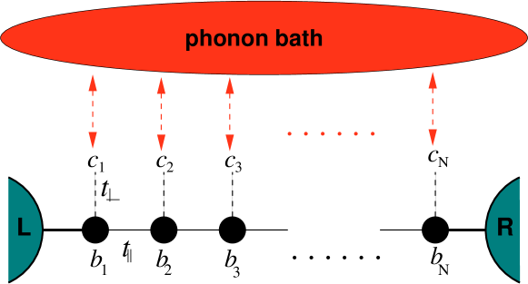
Figure 36: (Color) Schematic drawing of a DNA molecular wire in contact with a dissipative environment. The central chain (extended states) with $N$ sites is connected to semiinfinite left (L) and right (R) electronic reservoirs. The bath only interacts with the side chain sites (c), which we call for simplicity backbone sites, but which collectively stay for non-conducting, localized electronic states. The Hamiltonian associated with this model is given by Eqs. (443), (444), and (445) in the main text.

Hereby ${\cal H}_{\textrm{C}}$ and ${\cal H}_{\textrm{b}}$ are the Hamiltonians of the extended and localized states (called in what follows “backbone” states for simplicity), respectively, and ${\cal H}_{\textrm{C-b}}$ is the coupling between them. $t_{||}$ and $t_{\perp}$ are hopping integrals along the central chain (extended states) and between the localized states and the central chain, respectively. If not stated otherwise, the on-site energies will be later set equal to zero to simplify the calculations. Notice that this model displays a gap in the electronic spectrum roughly proportional to the transversal coupling $t_{\perp}$. This can be easely seen by looking at the limit $N\to\infty$ which leads to a periodic system. In this case, the Hamiltonian can be analytically diagonalized and two energy dispersion curves are obtained, which are given by $E_{\pm}(k)=t_{||}\cos(k)\pm\sqrt{t^{2}_{\perp}+t^{2}_{||}\cos^{2}(k)}$. The direct gap between the two bands is simply $\delta=2\sqrt{t^{2}_{\perp}+t^{2}_{||}}$. Since this model further shows electron-hole symmetry, two electronic manifolds (bands in the limit of $N\to\infty$) containing $N$ states each, are symmetrically situated around the Fermi level, which is taken as the zero of energy.

The gap is obviously temperature independent and furthermore it is expected that transport at energies $E<\delta$ will be strongly suppressed due to the absence of electronic states to suport charge propagation. As a result, the linear conductance should display a strong exponential dependence as a function of the chain length $N$. In view of this behavior, an immediate issue that arises is how stable this electronic structure, i.e. two electronic manifolds separated by a gap, is against the coupling to an environment. This is an issue which reaches farther than the problem of charge transport in DNA wires, since it addresses the interaction of an open quantum mechanical system with a countable number of electronic energy levels to a continuum of states (“universe”). A generic example of such a situation is the measurement process in quantum mechanics. It is well-known that the interaction with complex environments is a source of dissipation and decoherence in quantum mechanical systems. Weiss99book Concerning more specifically the case of DNA (and proteins), there is broad experimental evidence that the molecule dynamics follows the solvent dynamics over a broad temperature range. Especially, conformational changes, low-energy vibrational excitations and the corresponding temperature dependences turn out to be very sensitive to the solvents dynamics. Caliskan04jcp We will thus consider the vibrational degrees of freedom of counterions and hydration shells of the solvent as a dynamical bath able to break the electronic phase coherence and additionally to act as a dissipative environment. We do not consider specific features of the environment but represent it in a generic way by a bosonic bath of $M$ harmonic oscillators. Then, the previous Hamiltonian can be extended to:

$${\cal H}_{\textrm{W}}={\cal H}_{\textrm{el}}+\sum_{\alpha}\Omega_{\alpha}B^{\dagger}_{\alpha}B_{\alpha}+\sum_{\alpha,j}\lambda_{\alpha}c^{\dagger}_{j}c_{j}(B_{\alpha}+B^{\dagger}_{\alpha})={\cal H}_{\textrm{el}}+{\cal H}_{\textrm{B}}+{\cal H}_{\textrm{c-B}},$$ (444)

where ${\cal H}_{\textrm{B}}$ and ${\cal H}_{\textrm{c-B}}$ are the phonon bath Hamiltonian and the (localized) state-bath interaction, respectively. $B_{\alpha}$ is a bath phonon operator and $\lambda_{\alpha}$ denotes the electron-phonon coupling. Note that we assume a local coupling of the bath modes to the electronic density at the side chain. Later on, the thermodynamic limit ($M\to\infty)$ in the bath degrees of freedom will be carried out and the corresponding bath spectral density introduced, so that at this stage we do not need to further specify the set of bath frequencies $\Omega_{\alpha}$ and coupling constants $\lambda_{\alpha}$. Obviously, the bath can be assumed to be in thermal equilibrium and be described by a canonical partition function.

To complete the formulation of the model, we have to include the interaction of the system with electronic reservoirs in order to describe charge transport along the same lines as before. We assume, as usual, a tunnel-type Hamiltonian with the form:

$${\cal H} = {\cal H}_{\textrm{W}}+\sum_{{\bf k}\in\textrm{L,R},\sigma}\epsilon_{{\bf k}\sigma}d^{\dagger}_{{\bf k}\sigma}d_{{\bf k}\sigma}+\sum_{{\bf k}\in\textrm{L},\sigma}(V_{{\bf k},1}\,d^{\dagger}_{{\bf k}\sigma}\,b_{1}+\textrm{H.c.})$$ (445)

$$+\sum_{{\bf k}\in R,\sigma}(V_{{\bf k},N}\,d^{\dagger}_{{\bf k}\sigma}\,b_{N}+\textrm{H.c.})={\cal H}_{\textrm{W}}+{\cal H}_{\textrm{L/R}}+{\cal H}_{\textrm{L-C}}+{\cal H}_{\textrm{R-C}}.$$

The Hamiltonian of Eq. (445) is the starting point of our investigation. For a weak charge-bath coupling, a perturbative approach similar to the second order Born approximation, as described in the previous section can be applied. We expect, however, qualitative new effects rather in the opposite limit of strong coupling to the bath. To deal with this problem, a unitary transformation, the Lang-Firsov (LF) transformation, can be performed on the Hamiltonian of Eq. (445), which allows to eliminate the linear charge-vibron interaction ${\cal H}_{\textrm{c-B}}$. In the limiting case of an isolated system with a single electron (or hole) this transformation becomes exact and allows for a full decoupling of electronic and vibronic propagators, see e.g. Ref. Mahan90book . In the present case, this transformation is not exact and further approximations have to be introduced in order to make the problem tractable.

The generator of the LF transformation is given by

$$S=\sum_{\alpha,j}({\lambda_{\alpha}}/{\Omega_{\alpha}})c^{\dagger}_{j}c_{j}(B_{\alpha}-B^{\dagger}_{\alpha})$$

and $S^{\dagger}=-S$. In the transformed Hamiltonian $\bar{\cal{H}}=\textrm{e}\,^{S}{\cal{H}}\textrm{e}\,^{-S}$ the linear coupling to the bath is eliminated. One should notice that in $\bar{\cal{H}}$ only the “backbone” part of the Hamiltonian is modified since the conducting state operators $b_{\ell}$ as well as the lead operators $d_{\bf{k}\sigma}$ are invariant with respect to the above transformation. The new Hamiltonian reads:

$$\bar{{\cal H}} = {\cal H}_{\textrm{C}}+{\cal H}_{\textrm{L/R}}+{\cal H}_{\textrm{B}}+{\cal H}_{\textrm{L/R-C}}+(\epsilon-\Delta)\sum_{j}c^{\dagger}_{j}c_{j}-{t_{\perp}\sum_{j}\left[b^{\dagger}_{j}c_{j}{\cal X}+\textrm{H.c.}\right]},$$

$${\cal X} = \exp{\left[\sum_{\alpha}\frac{\lambda_{\alpha}}{\Omega_{\alpha}}(B_{\alpha}-B^{\dagger}_{\alpha})\right]},\;\;\;\Delta=\sum_{\alpha}\frac{\lambda_{\alpha}^{2}}{\Omega_{\alpha}}.$$ (446)

As a result of the LF we get a shift of the onsite energies (polaron shift or reorganization energy in electron transfer theory) and a renormalization of both the tunneling and of the transversal coupling Hamiltonian via the bosonic operators ${\cal X}$. There is also an additional electron-electron interaction term which we will not be concerned with in the remaining of this section and is thus omitted. Since we are mainly interested in qualitative statements, we will assume the wide-band approximation in the coupling to the electrodes which is equivalent to substituting the electrode self-energies by a purely imaginary constant, i.e. $\Sigma_{\rm L,R}\approx-\textrm{i}\,\Gamma_{\rm L,R}$. We are thus not interested in specific features of the electrode electronic structure.

To further proceed, let us now introduce two kinds of retarded thermal Green functions related to the central chain $G_{j\ell}(t)$ and to the “backbones” $P_{j\ell}(t)$, respectively (taking $\hbar=1$):

$$G_{j\ell}(t,t^{\prime}) = -i\Theta(t-t^{\prime})\left\langle\left[b_{j}(t),b^{\dagger}_{\ell}(t^{\prime})\right]_{+}\right\rangle,$$ (447)

$$P_{j\ell}(t,t^{\prime}) = -i\Theta(t-t^{\prime})\left\langle\left[c_{j}(t){\cal X}(t),c^{\dagger}_{\ell}(t^{\prime}){\cal X}^{\dagger}(t^{\prime})\right]_{+}\right\rangle,$$

where $\Theta$ is the Heaviside function. Notice that the $P$-Green function doe not have a pure electronic character but also contains the bath operators ${\cal X}$. For a full out-of-equilibrium calculation, the full Keldysh formalism including lesser- and greater-GF would also be needed. However, as we will briefly show below, the final expression for the electrical current at low applied voltages and for small transversal coupling $t_{\perp}$ will only include the retarded propagators.

We now use the equation of motion technique (EOM) to obtain an expression for the GF $G_{j\ell}(t)$. We first remark that in the time domain two EOM can be written, depending on which time argument in the double-time GF the time derivative will act. One thus obtains in general:

$$\textrm{i}\,\partial_{t}G(t,t^{\prime})=\left\langle\left[b(t),b^{\dagger}(t^{\prime})\right]_{+}\right\rangle\delta(t-t^{\prime})+((\left[b(t),H\right]|b^{\dagger}(t^{\prime}))).$$

$$G(t,t^{\prime})[-\textrm{i}\,\partial_{t^{\prime}}]=\left\langle\left[b(t),b^{\dagger}(t^{\prime})\right]_{+}\right\rangle\delta(t-t^{\prime})-((b(t)|\left[b^{\dagger}(t^{\prime}),H\right])).$$

The EOM for the GF $G_{j\ell}(t)$ reads then in the energy space:

$$\sum_{n}\left[G^{-1}_{0}(E)\right]_{\ell n}G_{nj}(E)=\delta_{\ell j}-t_{\perp}((c_{\ell}{\cal X}|b^{\dagger}_{j}))$$ (448)

$$\Big{[}G^{-1}_{0}(E)\Big{]}_{\ell n} = (E-\epsilon_{b})\delta_{n\ell}+t_{||}(\delta_{n,\ell+1}+\delta_{n,\ell-1})-\Sigma_{\textrm{L}}\delta_{\ell 1}\delta_{n1}-\Sigma_{\textrm{R}}\delta_{\ell N}\delta_{nN}$$

$$\Sigma_{\textrm{L(R)}} = \sum_{{\bf k}\in L(R)}\frac{|V_{{\bf k},1(N)}|^{2}}{E-\epsilon_{{\bf k}}+\textrm{i}\,0^{+}}\approx-\textrm{i}\,\Gamma_{\rm L,R}$$

In the next step, EOM for the “right” time argument $t^{\prime}$ of the GF $Z_{\ell j}^{{\cal X}}(t,t^{\prime})((c_{\ell}(t){\cal X}(t)|b^{\dagger}_{j}(t^{\prime})))$ can be written. This leads to:

$$\sum_{m}Z_{\ell m}^{{\cal X}}(E)\left[G^{-1}_{0}(E)\right]_{mj}=-t_{\perp}((c_{\ell}{\cal X}|c^{\dagger}_{j}{\cal X}^{\dagger}))=-t_{\perp}P_{\ell j}(E)$$ (449)

Inserting Eq. (449) into Eq. (448) we arrive at the matrix equation:

$${\bf G}(E)={\bf G}_{0}(E)+{\bf G}_{0}(E){\bf\Sigma}_{\textrm{B}}(E){\bf G}_{0}(E),$$

which can be transformed into a Dyson-like equation when introducing the irreducible part ${\bf\Sigma}_{\textrm{B}}(E)={\bf\Sigma}^{\textrm{irr}}_{\textrm{B}}(E)+{\bf\Sigma}^{\textrm{irr}}_{\textrm{B}}(E){\bf G}_{0}(E){\bf\Sigma}^{\textrm{irr}}_{\textrm{B}}(E)+\dots$:

$${\bf G}(E)={\bf G}_{0}(E)+{\bf G}_{0}(E){\bf\Sigma}^{\textrm{irr}}_{\textrm{B}}(E){\bf G}(E),$$ (450)

or equivalently:

$${\bf G}^{-1}(E) = {\bf G}_{0}^{-1}(E)-t^{2}_{\perp}{\bf P}(E)$$ (451)

$${\bf G}_{0}^{-1}(E) = E{\bf 1}-{\cal H}_{\textrm{C}}-\Sigma_{\textrm{L}}(E)-\Sigma_{\textrm{R}}(E).$$

${\bf\Sigma}^{\textrm{irr}}_{\textrm{B}}(E)=t^{2}_{\perp}{\bf P}(E)$ is the crucial contribution to the GF since it contains the influence of the bosonic bath. Note that ${\bf\Sigma}^{\textrm{irr}}_{\textrm{B}}(E)$ includes the transversal hopping $t_{\perp}$ to all orders, the leading one being $t^{2}_{\perp}$.

In the next step, an expression for the electrical current flowing through the system must be derived. Using the results of Sec. 2, we can directly write the following expression:

$$I=\frac{2e}{h}\int dE\,\textrm{Tr}(f_{\rm L}(E)-f_{\rm R}(E))\;t(E)$$

$$+t^{2}_{\perp}\frac{2e}{h}\int dE\,\left\{\textrm{Tr}[{\bf\Sigma}^{>}_{\rm L}\,{\bf P}^{<}-{\bf\Sigma}^{<}_{\rm L}\,{\bf P}^{>}]-(L\leftrightarrow R)\right\}.$$ (452)

The first summand has the same form as Landauer’s expression for the current with an effective transmission function $t(E)=\textrm{Tr}[{\bf G}^{\dagger}{\bf\Gamma}_{\rm R}{\bf G}{\bf\Gamma}_{\rm R}]$. However, the reader should keep in mind that the GFs appearing in this expression do contain the full dressing by the bosonic bath and hence, $t(E)$ does not describe elastic transport. The remaining terms contain explicitly contributions from the bath. It can be shown after some transformations that the leading term is proportional to $(t^{2}_{\perp})^{2}$ so that within a perturbative approach in $t_{\perp}$ and at low bias it can be approximately neglected. We therefore remian with the exression $I=\frac{2e}{h}\int dE\,\textrm{Tr}(f_{\rm L}(E)-f_{\rm R}(E))\;t(E)$ to obtain the current.

To remain consistent with this approximation, the bath selfenergy should also be treated to order $t^{2}_{\perp}$, more explicitly:

$$P_{\ell j}(t,t^{\prime})=((c_{\ell}(t){\cal X}(t)|c^{\dagger}_{j}(t^{\prime}){\cal X}^{\dagger}(t^{\prime})))$$

$$\approx-\textrm{i}\,\theta(t-t^{\prime})\left\{\left\langle c_{\ell}(t)c^{\dagger}_{j}(t^{\prime})\right\rangle\left\langle{\cal X}(t){\cal X}^{\dagger}(t^{\prime})\right\rangle+\left\langle c^{\dagger}_{j}(t^{\prime})c_{\ell}(t)\right\rangle\left\langle{\cal X}^{\dagger}(t^{\prime}){\cal X}(t)\right\rangle\right\}$$

$$\approx-\textrm{i}\,\delta_{\ell j}\theta(t-t^{\prime})\left\{\left\langle c_{j}(t)c^{\dagger}_{j}(t^{\prime})\right\rangle\left\langle{\cal X}(t){\cal X}^{\dagger}(t^{\prime})\right\rangle+\left\langle c^{\dagger}_{j}(t^{\prime})c_{j}(t)\right\rangle\left\langle{\cal X}^{\dagger}(t^{\prime}){\cal X}(t)\right\rangle\right\}$$

$$=-\textrm{i}\,\delta_{\ell j}\theta(t-t^{\prime})\textrm{e}\,^{-{\textrm{i}\,}(\epsilon-\Delta)\,t}\left\{(1-f_{\sf c})\textrm{e}\,^{-\Phi(t)}+f_{\sf c}\textrm{e}\,^{-\Phi(-t)}\right\}.$$ (453)

In the previous expression we have replaced the full averages of the “backbone” operators by their zero order values (free propagators). $\textrm{e}\,^{-\Phi(t)}=\left\langle{\cal X}(t){\cal X}^{\dagger}(0)\right\rangle_{\textrm{B}}$ is a dynamical bath correlation function to be specified later on. The average $\left\langle\cdot\right\rangle_{\textrm{B}}$ is performed over the bath degrees of freedom. $f_{\sf c}$ is the Fermi function at the backbone sites. In what follows we consider the case of empty sites by setting $f_{\sf c}=0$. The Fourier transform $P_{\ell j}(E)$ reads then:

$$P_{\ell j}(E)=-\textrm{i}\,\delta_{\ell j}\int_{0}^{\infty}\mathrm{d}t\,\textrm{e}\,^{{\textrm{i}\,}(E+{\textrm{i}\,}0^{+})t}\,\textrm{e}\,^{-{\textrm{i}\,}(\epsilon-\Delta)\,t}\,\;\left[(1-f_{\sf c})\textrm{e}\,^{-\Phi(t)}+f_{\sf c}\textrm{e}\,^{-\Phi(-t)}\right]$$ (454)

In order to get closed expressions for the bath thermal averages it is appropriate to introduce a bath spectral density Weiss99book defined by :

$$J(\omega)=\sum_{\alpha}\lambda^{2}_{\alpha}\delta(\omega-\Omega_{\alpha})=J_{0}(\frac{\omega}{\omega_{\textrm{c}}})^{s}\textrm{e}\,^{-\omega/\omega_{\textrm{c}}}\Theta(\omega),$$ (455)

where $\omega_{\textrm{c}}$ is a cut-off frequency related to the bath memory time $\tau_{\textrm{c}}\sim\omega_{\textrm{c}}^{-1}$. It is easy to show that the limit $\omega_{\textrm{c}}\to\infty$ corresponds to a Markovian bath, i.e.  $J(t)\sim J_{0}\delta(t)$. Using this Ansatz, $\Phi(t)$ can be written as:

$$\Phi(t) = \int_{0}^{\infty}\mathrm{d}\omega\,\frac{J(\omega)}{\omega^{2}}\left[1-\textrm{e}\,^{-{\textrm{i}\,}\omega t}+2\frac{1-\cos{\omega t}}{\textrm{e}\,^{\beta\omega}-1}\right].$$ (456)

Although the integral can be performed analytically Weiss99book , we consider $\Phi(t)$ in some limiting cases where it is easier to work directly with Eq. (456).

Limiting cases

We use now the results of the foregoing section to discuss the electronic transport properties of our model in some limiting cases for which analytic expressions can be derived. We will discuss the mean-field approximation and the weak-coupling regime in the electron-bath interaction as well as to elaborate on the strong-coupling limit. Farther, the cases of ohmic ($s=1$) and superohmic ($s=3$) spectral densities are treated.

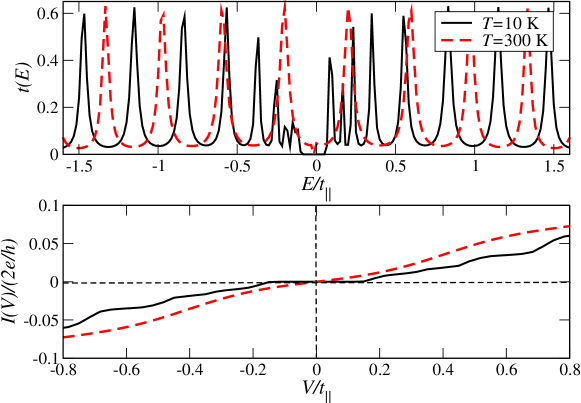
Figure 37: (Color) Electronic transmission and corresponding current in the mean-field approximation for two different temperatures. Parameters: $N=20,J_{0}/\omega_{\textrm{c}}=0.12,t_{\perp}/t_{||}=0.5,\Gamma_{\textrm{L/R}}/t_{||}=0.5$.

(i) Mean-field approximation

The mean-field approximation is the simplest one and neglects bath fluctuations contained in $P(E)$. The MFA can be introduced by writing the phonon operator ${\cal X}$ as $\left\langle{\cal X}\right\rangle_{\rm B}+\delta{\cal X}$ in ${\cal H}_{\textrm{C-c}}$ in Eq. (4.3), i.e. ${\cal H}^{\textrm{MF}}_{\textrm{C-b}}=-t_{\perp}\sum_{j}\left[b^{\dagger}_{j}c_{j}\left\langle{\cal X}\right\rangle_{\textrm{B}}+\textrm{H.c.}\right]+O(\delta{\cal X})$. As a result a real, static and temperature dependent term in Eq. (451) is found:

$${\bf G}^{-1}(E)={\bf G}_{0}^{-1}(E)-t^{2}_{\perp}\frac{|\left\langle{\cal X}\right\rangle_{\textrm{B}}|^{2}}{E-\epsilon+\Delta+\textrm{i}\,0^{+}}{\bf 1},$$ (457)

where $\left|\left\langle{\cal X}\right\rangle_{\textrm{B}}\right|^{2}=\textrm{e}\,^{-2\kappa(T)}$ and $\kappa(T)$ is given by:

$$\kappa(T)=\int_{0}^{\infty}\frac{\mathrm{d}\omega}{\omega^{2}}J(\omega)\coth{\frac{\omega}{2k_{\textrm{B}}T}}.$$ (458)

The effect of the MF term is thus to scale the bare transversal hopping $t_{\perp}$ by the exponential temperature dependent factor $\textrm{e}\,^{-\kappa(T)}$.

In the case of an ohmic bath, $s=1$, the integrand in $\kappa(T)$ scales as $1/\omega^{p},\,p=1,2$ and has thus a logarithmic divergence at the lower integration limit. Thus, the MF contribution would vanish. In other words, no gap would exist on this approximation level.

In the superohmic case ($s=3$) all integrals are regular. One obtains $\Delta=\int\mathrm{d}\omega\,\omega^{-1}J(\omega)=\Gamma(s-1)J_{0}=2J_{0}$, with $\Gamma(s)$ being the Gamma function and $\kappa(T)$ reads:

$$\kappa(T)=\frac{2J_{0}}{\omega_{\textrm{c}}}\left[\,2\left(\frac{k_{\textrm{B}}T}{\omega_{\textrm{c}}}\right)^{2}\,\zeta_{\textrm{H}}\left(2,\frac{k_{\textrm{B}}T}{\omega_{\textrm{c}}}\right)-1\right].$$ (459)

$\zeta_{\textrm{H}}(s,z)=\sum_{n=0}^{\infty}(n+z)^{-s}$ is the Hurwitz $\zeta$-function, a generalization of the Riemann $\zeta$-function. Gradshteyn00book

It follows from Eq. (17) that $\kappa(T)$ behaves like a constant for low temperatures ($k_{\textrm{B}}T/\omega_{\textrm{c}}<1$), $\kappa(T)\sim J_{0}/\omega_{\textrm{c}}$, while it scales linear with $T$ in the high-temperature limit ($k_{\textrm{B}}T/\omega_{\textrm{c}}>1$), $\kappa(T)\sim J_{0}/\omega_{\textrm{c}}(1+2k_{\textrm{B}}T/\omega_{\textrm{c}})$).

For $J_{0}\neq 0$ and at zero temperature the hopping integral is roughly reduced to $t_{\perp}\textrm{e}\,^{-\frac{J_{0}}{\omega_{\textrm{c}}}}$ which is similar to the renormalization of the hopping in Holstein’s polaron model Holstein59apny , though here it is $t_{\perp}$ rather than $t_{||}$ the term that is rescaled. At high temperatures $t_{\perp}$ is further reduced ($\kappa(T)\sim T$) so that the gap in the electronic spectrum finally collapses and the system becomes “metallic”, see Fig. 37. An appreciable temperature dependence can only be observed in the limit $J_{0}/\omega_{\textrm{c}}<1$; otherwise the gap would collapse already at zero temperature due to the exponential dependence on $J_{0}$. We further remark that the MFA is only valid in this regime ($J_{0}/\omega_{\textrm{c}}<1$), since for $J_{0}/\omega_{\textrm{c}}\gg 1$ multiphonon processes in the bath, which are not considered in the MFA, become increasingly relevant and thus a neglection of bath fluctuations is not possible.

(ii) Beyond MF: weak-coupling limit

As a first step beyond the mean-field approach let’s first consider the weak-coupling limit in ${\bf P}(E)$. For $J_{0}/\omega_{\textrm{c}}<1$ and not too high temperatures ($k_{\textrm{B}}T/\omega_{\textrm{c}}<1$) the main contribution to the integral in Eq. (456) comes from long times $t\gg\omega_{\textrm{c}}^{-1}$.

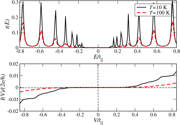
Figure 38: (Color) Electronic transmission and corresponding current in the weak-coupling limit with ohmic dissipation ($s=1$) in the bath. Parameters: $N=20,J_{0}/\omega_{\textrm{c}}=0.2,t_{\perp}/t_{||}=0.6,\Gamma_{\textrm{L/R}}/t_{||}=0.5$

With the change of variables $z=\omega t$, $\Phi(t)$ can be written as:

$$\Phi(t) = J_{0}\omega_{\textrm{c}}^{-s}t^{1-s}\int_{0}^{\infty}\mathrm{d}z\,z^{s-2}\textrm{e}\,^{-\frac{z}{\omega_{\textrm{c}}t}}$$ (460)

$$\times\left(1-\textrm{e}\,^{-\textrm{i}\,z}+2\frac{1-\cos{z}}{\textrm{e}\,^{z\frac{\beta\omega_{\textrm{c}}}{\omega_{\textrm{c}}t}}-1}\right).$$

As far as $\omega_{\textrm{c}}t\gg\beta\omega_{\textrm{c}}$ this can be simplified to:

$$\Phi(t) \approx J_{0}\omega_{\textrm{c}}^{-s}t^{1-s}\int_{0}^{\infty}\mathrm{d}x\,z^{s-2}\textrm{e}\,^{-\frac{z}{\omega_{\textrm{c}}t}}$$ (461)

$$\times\left(1-\textrm{e}\,^{-\textrm{i}\,z}+2\frac{\beta\omega_{\textrm{c}}}{\omega_{\textrm{c}}t}\frac{1-\cos{z}}{z}\right).$$

Since in the long-time limit the low-frequency bath modes are giving the most important contribution we may expect some qualitative differences in the ohmic and superohmic regimes. For $s=1$ we obtain $\Phi(t)\sim\pi\frac{J_{0}}{\omega_{\textrm{c}}}\frac{k_{\textrm{B}}T}{\omega_{\textrm{c}}}(\omega_{\textrm{c}}t)$ which leads to ($\Delta(s=1)=J_{0}$):

$${\bf G}^{-1}(E) = {\bf G}_{0}^{-1}(E)-t^{2}_{\perp}\frac{1}{E+J_{0}+\textrm{i}\,\pi\frac{J_{0}}{\omega_{\textrm{c}}}k_{\textrm{B}}T}{\bf 1},$$ (462)

i.e. there is only a pure imaginary contribution from the bath. For the simple case of $N=1$ (a two-states model) one can easily see that the gap approximately scales as $\sqrt{k_{\textrm{B}}T}$; thus it grows with increasing temperature. This is shown in Fig. 38, where we also see that the intensity of the transmission resonances strongly goes down with increasing temperature. The gap enhancement is induced by the suppression of the transmission peaks of the frontier orbitals, i. e. those closest to the Fermi energy.

For $s=3$ and $k_{\textrm{B}}T/\omega_{\textrm{c}}<1$, $\Phi(t)$ takes a nearly temperature independent value proportional to $J_{0}/\omega_{\textrm{c}}$. As a result the gap is slightly reduced ($t_{\perp}\to t_{\perp}\textrm{e}\,^{-J_{0}/\omega_{\textrm{c}}}$) but, because of the weak-coupling condition, the effect is rather small.
From this discussion we can conclude that in the weak-coupling limit ohmic dissipation in the bath induces an enhancement of the electronic gap while superohmic dissipation does not appreciably affect it. In the high-temperature limit $k_{\textrm{B}}T/\omega_{\textrm{c}}>1$ a short-time expansion can be performed which yields similar results to those of the strong-coupling limit (see next section), Ao96prb so that we do not need to discuss them here. Note farther that the gap obtained in the weak-coupling limit is an “intrinsic” property of the electronic system; it is only quantitatively modified by the interaction with the bath degrees of freedom. We thus trivially expect a strong exponential dependence of $t(E=E_{{\rm F}})$, typical of virtual tunneling through a gap. Indeed, we find $t(E=E_{{\rm F}})\sim\exp{(-\beta\,L)}$ with $\beta\sim 2-3\,\AA^{-1}$.

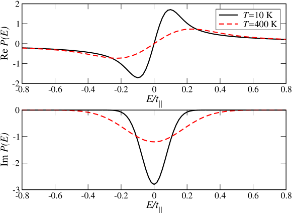
Figure 39: (Color) Temperature dependence of the real and imaginary parts of $P(E)$ for $N=20$, $J_{0}/\omega_{\textrm{c}}=10,t_{\perp}/t_{||}=0.4,\Gamma_{\textrm{L/R}}/t_{||}=0.5$. With increasing temperature the slope of the real part near $E=0$ decreases and the imaginary part broadens and loses intensity. A similar qualitative dependence on $J_{0}$ was found (not shown).

(iii) Beyond MF: strong coupling limit (SCL)

In this section we elaborate on the strong-coupling regime, as defined by the condition $J_{0}/\omega_{\textrm{c}}>1$. In the SCL the main contribution to the time integral in Eq. (456) arises from short times. Hence a short-time expansion of $\Phi(t)$ may already give reasonable results and it allows, additionally, to find an analytical expression for ${\bf P}(E)$. At $t\ll\omega_{\textrm{c}}^{-1}$ we find,

$$\Phi(t) \approx {\textrm{i}\,}\Delta\,t+(\omega_{\textrm{c}}t)^{2}\,\kappa_{0}(T)$$ (463)

$$P_{\ell j}(E) = -{\textrm{i}\,}\delta_{\ell j}\,\,\int_{0}^{\infty}\mathrm{d}t\,\textrm{e}\,^{{\textrm{i}\,}(E-\epsilon+{\textrm{i}\,}0^{+})t}\,\textrm{e}\,^{-(\omega_{\textrm{c}}t)^{2}\kappa_{0}(T)}$$

$$= -{\textrm{i}\,}\delta_{\ell j}\,\,\frac{\sqrt{\pi}}{2}\frac{1}{\omega_{\textrm{c}}\sqrt{\kappa_{0}(T)}}\;\exp\left({-\frac{(E-\epsilon+{\textrm{i}\,}0^{+})^{2}}{4\omega^{2}_{\textrm{c}}\kappa_{0}(T)}}\right)$$

$$\times\left(1+{\textrm{erf}}\left[\frac{{\textrm{i}\,}(E-\epsilon+{\textrm{i}\,}0^{+})}{2\omega_{\textrm{c}}\sqrt{\kappa_{0}(T)}}\right]\right),$$

$$\kappa_{0}(T) = \frac{1}{2\omega^{2}_{\textrm{c}}}\int_{0}^{\infty}\mathrm{d}\omega J(\omega)\coth{\frac{\omega}{2k_{\textrm{B}}T}}.$$

Before presenting the results for the electronic transmission, it is useful to first consider the dependence of the real and imaginary parts of ${\bf P}(E)$ on temperature and on the reduced coupling constant $J_{0}/\omega_{\textrm{c}}$. Both functions are shown in Fig. 39. We see that around the Fermi level at $E=0$ the real part is approximately linear, ${\rm Re}\,P(E)\sim E$ while the imaginary part shows a Lorentzian-like behavior. The imaginary part loses intensity and becomes broadened with increasing temperature or $J_{0}$, while the slope in the real part decreases when $k_{\textrm{B}}T$ or $J_{0}$ are increased.

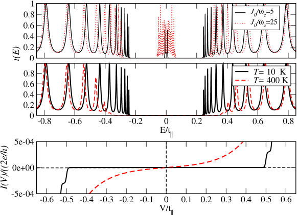
Figure 40: (Color) Upper panel: $t(E)$ with ${\rm{Im}}\,P(E)=0$; the intensity of the resonances on the central narrow band is strongly dependent on $J_{0}/\omega_{c}$ and $k_{\textrm{B}}T$ (not shown). Temperature dependence of $t(E)$ with full inclusion of $P(E)$ (middle panel) and corresponding current (lower panel) for $N=20$, $J_{0}/\omega_{\textrm{c}}=5,t_{\perp}/t_{||}=0.5,\Gamma_{\textrm{{L/R}}}/t_{||}=0.2$. The pseudo-gap increases with temperature.

If we neglect for the moment the imaginary part (the dissipative influence of the bath), we can understand the consequences of the real part being nonzero around the Fermi energy, i.e. in the gap region of the model of Ref. Cuniberti02prb . The solutions of the non-linear equation ${\rm{det}}|(E-t_{\perp}^{2}{\rm Re}\,P(E)){\bf 1}-{\cal H}_{\textrm{C}}|=0$ give the new poles of the Green function of the system in presence of the phonon bath. For comparison, the equation determining the eigenstates without the bath is simply ${\rm{det}}|(E-t_{\perp}^{2}/E){\bf 1}-{\cal H}_{\textrm{C}}|=0$. It is just the $1/E$ dependence near $E=0$ that induces the appearance of two electronic bands of states separated by a gap. In our present study, however, ${\rm Re}\,P(E\to 0)$ has no singular behavior and additional poles of the Green function may be expected to appear in the low-energy sector. This is indeed the case, as shown in Fig. 40 (upper panel). We find a third band of states around the Fermi energy, which we may call a polaronic band because it results from the strong interaction between an electron and the bath modes. The intensity of this band as well as its band width strongly depend on temperature and on $J_{0}$. When $k_{\textrm{B}}T$ (or $J_{0}$) become large enough, these states spread out and eventually merge with the two other side bands. This would result in a transmission spectrum similar of a gapless system.

This picture is nevertheless not complete since the imaginary component of $P(E)$ has been neglected. Its inclusion leads to a dramatic modification of the spectrum, as shown in Fig. 40 (middle panel). We now only see two bands separated by a gap which basically resembles the semiconducting-type behavior of the original model. The origin of this gap or rather pseudo-gap (see below) is however quite different. It turns out that the imaginary part of $P(E)$, being peaked around $E=0$, strongly suppresses the transmission resonances belonging to the third band. Additionally, the frontier orbitals on the side bands, i.e.  orbitals closest to the gap region, are also strongly damped, this effect becoming stronger with increasing temperature (${\rm{Im}}\,P(E)$ broadens). This latter effect has some similarities with the previously discussed weak-coupling regime. Note, however, that the new electronic manifold around the Fermi energy does not appear in the weak-coupling regime. We further stress that the density of states around the Fermi level is not exactly zero (hence the term pseudo-gap); the states on the polaronic manifold, although strongly damped, contribute nevertheless with a finite temperature dependent background to the transmission. As a result, with increasing temperature, a crossover from “semiconducting” to “metallic” behavior in the low-voltage region of the $I$-$V$ characteristics takes place, see Fig. 40 (lower panel). The slope in the $I$-$V$ plot becomes larger when $t_{\perp}$ is reduced, since the side bands approach each other and the effect of ${\rm{Im}}\,P(E)$ is reinforced.

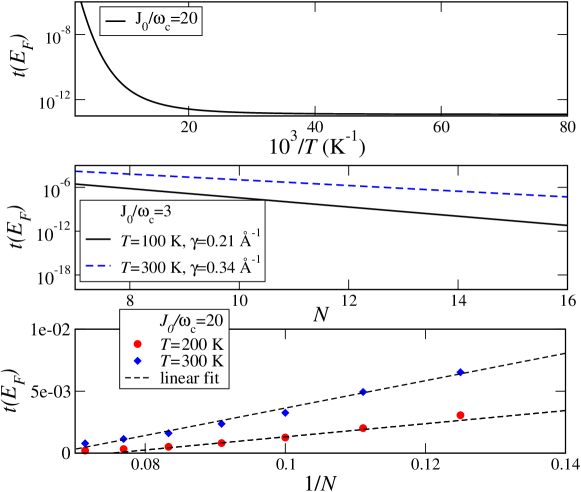
Figure 41: (Color) Upper panel: Arrhenius plot for $t(E_{F})$. Parameters: $N=20,\,t_{||}=0.6\,eV,\,t_{\perp}/t_{||}=0.2,\,\Gamma_{\textrm{{L/R}}}/t_{||}=0.3$. Middle and lower panels: Length dependence of $t(E_{F})$ at different temperatures for two different strengths of the electron-bath coupling $J_{0}/\omega_{\rm c}$. The electronic coupling parameters are the same as in the upper panel.

In Fig. 41 (top panel) an Arrhenius plot of the transmission at the Fermi energy is shown, which suggests that activated transport is the physical mechanism for propagation at low energies. Increasing the coupling to the phonon bath makes the suppression of the polaronic band around $E=0$ less effective (${\rm{Im}}\,P(E\sim 0)$ decreases) so that the density of states around this energy becomes larger. Hence the absolute value of the transmission will also increase. On the other side, increasing $t_{\perp}$ leads to a reduction of the transmission at the Fermi level, since the energetic separation of the side bands increases with $t_{\perp}$.

A controversial issue in transport through molecular wires is the actual length dependence of the electron transfer rates or correspondingly, of the linear conductance. This is specially critical in the case of DNA nanowires Treadway02chemphys ; Meggers98jacs ; Kelley99science . Different functional dependences have been found in charge transfer experiments ranging from strong exponential behavior related to superexchange mediated electron transfer Meggers98jacs to algebraic dependences typical of thermal activated hopping Treadway02chemphys ; Kelley99science . As far as transport experiments are concerned, the previously mentioned experiments at the group of N. Tao Xu04nanolett reported an algebraic length dependence of the conductance for poly(GC) oligomers in solution. We have investigated the length dependence of $t(E_{F})$ and found for the strong dissipative regime $J_{0}/\omega_{\rm c}>1$, an exponential law for energies close to $E_{\rm F}$, $t(E_{\rm F})\sim\exp(-\gamma N)$. At the first sight, this might be not surprising since a gap in the spectrum does exist. Indeed, in the absence of the bath, i.e. with an intrinsic gap, we get decay lengths $\gamma_{{\rm coh}}$ of the order of 2 $\,{\rm\AA}^{-1}$. However, as soon as the interaction with the bath is included, we find values of $\gamma$ much smaller than expected for virtual tunneling, ranging from $0.15\,{\rm\AA}^{-1}$ to $0.4\,{\rm\AA}^{-1}$. Additionally, $\gamma$ is strongly dependent on the strength of the electron-bath coupling $J_{0}/\omega_{\textrm{c}}$ as well as on temperature; $\gamma$ is reduced when $J_{0}/\omega_{\textrm{c}}$ or $k_{\rm B}T$ increases, since in both cases the density of states within the pseudo-gap increases. Remarkably, a further increase of the electron-bath coupling eventually leads to an algebraic length dependence, see lower panel of Fig.  41.

The studies presented in this section indicate that the presence of a complex environment, which induces decoherence and dissipation, can dramatically modify the electronic response of a nanowire coupled to electrodes. Electron transport on the low-energy sector of the transmission spectrum is supported by the formation of (virtual) polaronic states. Though strongly damped, these states manifest nonetheless with a finite density of states inside the bandgap and mediate thermally activated transport.

5 Conclusions and Perspectives

In this chapter we have reviewed the method of nonequilibrium Green functions and few selected applications to problems related with charge transport at the molecular scale. Hereby we have only focused on minimal model Hamiltonian formulations which build a very appropriate starting point to illustrate the power and range of validity of such techniques. We have showed how this approach can be used to deal with a variety of physical systems, covering both noninteracting and interacting cases. Thus, so different issues as coherent transport, Coulomb blockade phenomena, charge-vibron interaction, coupling to dissipative environments, and the Kondo effect (not addressed in this review) can be in principle treated on the same footing. Specially, the existence of well-developed diagrammatic techniques allows for a systematic treatment of interactions in nanoscale quantum systems. For the sake of space, we did not deal with applications of NGF techniques to spin-dependent transport, a field that has been increasingly attracting the attention of the physical community in the past years due to its potential applications in quantum information theory and quantum computation Nielsen00book ; Bouwmeester00book . For the same reason, the implementation of NGF into first-principle based approaches was not discussed neither. This is nevertheless a crucial methodological issue, since system-specific and realistic information about molecule-metal contact details, charge transfer effects, modifications of the molecular electronic structure and configuration upon contacting, the electrostatic potential distribution in a device, etc can only be obtained via a full ab initio description of transport. For charge transport through noninteracting systems this has been accomplished some years ago by combining NGF with DFT methods. The inclusion of interactions, however, represents a much stronger challenge and has been mainly carried out, within the self-consistent Born-approximation, for the case of tunneling charges coupling to vibrational excitations in the molecular region. Also there were some efforts to include dynamical correlations into DFT-based approach. Much harder and till the present not achieved at all is the inclusion of electronic correlation effects, responsible for many-particle effects like Coulomb blockade or the Kondo effect, in a non-equilibrium transport situation. DFT-based techniques, being essentially mean-field theories, cannot deal in a straightforward way with such problems and have to be improved, e.g. within the LDA+U approaches. For the case of equilibrium transport, a generalization of the Landauer formula including correlations has been recently formulated as well as first attempts to go beyond the linear response regime; for strong out-of-equilibrium situations this will be, in our view, one of the most demanding issues that the theoretical “transport” community will be facing in the coming years.

6 Acknowledgments

The authors acknowledge the collaboration with Miriam del Valle, Marieta Gheorghe, Michael Hartung, Sudeep Mandal, and Soumya Mohapatra, with whom part of the work reviewed here was done. We appreciate very useful and illuminating discussions with Andrea Donarini, Pino D’Amico, Dietrich Förster, Milena Grifoni, Joachim Keller, Abraham Nitzan, Norbert Nemec, Danny Porath, Florian Pump, Klaus Richter, Eugen Starikow, and Juyeon Yi. We thank Antti-Pekka Jauho, Alessandro Pecchia, Tomáš Novotný, Hassan Raza, and Kristian Thygesen for their comments.

Funding by the EU through grant FET-IST-2001-38951 (international collaboration ”DNA-based nanoelectronic devices (DNAnanoDEVICES)”), by the DFG through grant CU 44/3-2 (international collaboration ”Single molecule based memories”), by the Volkswagen Stiftung under Grant No. I/78 340, by the DFG Graduated School “Nonlinearity and Nonequilibrium in Condensed Matter” GRK-638, by the DFG Priority Program “Quantum Transport at the Molecular Scale” SPP1243, and by Collaborative Research Center SFB 689 is acknowledged. We also thank the Vielberth Foundation, the Minerva Foundation, the German Exchange Program (DAAD), the Humboldt foundation, and the German-Israeli foundation (GIF) for financial support.

References

- (1) M.A. Reed, J.M. Tour, Sci. Am. 282, 86 (2000)
- (2) C. Joachim, J.K. Gimzewski, A. Aviram, Nature 408, 541 (2000)
- (3) M.A. Ratner, Mater. today 5, 20 (2002)
- (4) A. Nitzan, M.A. Ratner, Science 300, 1384 (2003)
- (5) G. Cuniberti, G. Fagas, K. Richter (eds.), Introducing Molecular Electronics, Lecture Notes in Physics, vol. 680 (Springer-Verlag, 2005)
- (6) C. Joachim, M.A. Ratner, PNAS 102, 8801 (2005)
- (7) A. Aviram, M.A. Ratner, Chem. Phys. Lett. 29, 277 (1974)
- (8) M.A. Reed, C. Zhou, C.J. Muller, T.P. Burgin, J.M. Tour, Science 278, 252 (1997)
- (9) J. Chen, M.A. Reed, A.M. Rawlett, J.M. Tour, Science 286, 1550 (1999)
- (10) H. Park, J. Park, A.K.L. Lim, E.H. Anderson, A.P. Alivisatos, P.L. McEuen, Nature 407, 57 (2000)
- (11) J. Park, A.N. Pasupathy, J.I. Goldsmit, C. Chang, Y. Yaish, J.R. Petta, M. Rinkoski, J.P. Sethna, H.D. Abruna, P.L. McEuen, D.C. Ralph, Nature 417, 722 (2002)
- (12) W. Liang, M.P. Shores, M. Bockrath, J.R. Long, H. Park, Nature 417, 725 (2002)
- (13) R.H.M. Smit, Y. Noat, C. Untiedt, N.D. Lang, M.C. van Hemert, J.M. van Ruitenbeek, Nature 419, 906 (2002)
- (14) J. Kushmerick, J. Lazorcik, C. Patterson, R. Shashidhar, D. Seferos, G. Bazan, Nano Letters 4, 639 (2004)
- (15) L.H. Yu, D. Natelson, Nano Lett. 4, 79 (2004)
- (16) L.H. Yu, Z.K. Keane, J.W. Ciszek, L. Cheng, M.P. Stewart, J.M. Tour, D. Natelson, Phys. Rev. Lett. 93, 266802 (2004)
- (17) X. Xiao, B. Xu, N.J. Tao, Nano Lett. 4, 267 (2004)
- (18) M. Elbing, R. Ochs, M. Koentopp, M. Fischer, C. von Hänisch, F. Weigend, F. Evers, H.B. Weber, M. Mayor, PNAS 102, 8815 (2005)
- (19) L. Venkataraman, J.E. Klare, I.W. Tam, C. Nuckolls, M.S. Hybertsen, M.L. Steigerwald, Nano Lett. 6, 458 (2006)
- (20) M. Poot, E. Osorio, K. O’Neill, J.M. Thijssen, D. Vanmaekelbergh, C.A. van Walree, L.W. Jenneskens, H.S.J. van der Zant, Nano Lett. 6, 1031 (2006)
- (21) E.A. Osorio, K. O’Neill, N. Stuhr-Hansen, O.F. Nielsen, T. Bj rnholm, H.S.J. van der Zant, Adv. Mater. 19, 281 (2007)
- (22) E. Lörtscher, H.B. Weber, H. Riel, Phys. Rev. Lett. 98, 176807 (2007)
- (23) D. Porath, Y. Levi, M. Tarabiah, O. Millo, Phys. Rev. B 56, 9829 (1997)
- (24) B.C. Stipe, M.A. Rezaei, W. Ho, S. Gao, M. Persson, B.I. Lundqvist, Phys. Rev. Lett. 78, 4410 (1997)
- (25) J.R. Hahn, W. Ho, Phys. Rev. Lett. 87, 196102 (2001)
- (26) Y. Kim, T. Komeda, M. Kawai, Phys. Rev. Lett. 89, 126104 (2002)
- (27) W. Ho, J. Chem. Phys. 117, 11033 (2002)
- (28) N. Nilius, T.M. Wallis, W. Ho, Science 297, 1853 (2002)
- (29) N. Nilius, T.M. Wallis, M. Persson, W. Ho, Phys. Rev. Lett. 90, 196103 (2003)
- (30) S.W. Hla, K.F. Braun, B. Wassermann, K.H. Rieder, Phys. Rev. Lett. 93, 208302 (2004)
- (31) N. Liu, N.A. Pradhan, W. Ho, J. Chem. Phys. 120, 11371 (2004)
- (32) X.H. Qiu, G.V. Nazin, W. Ho, Phys. Rev. Lett. 92, 206102 (2004)
- (33) S.W. Wu, G.V. Nazin, X. Chen, X.H. Qiu, W. Ho, Phys. Rev. Lett. 93, 236802 (2004)
- (34) J. Repp, G. Meyer, F.E. Olsson, M. Persson, Science 305, 493 (2004)
- (35) J. Repp, G. Meyer, S.M. Stojković, A. Gourdon, C. Joachim, Phys. Rev. Lett. 94, 026803 (2005)
- (36) J. Repp, G. Meyer, S. Paavilainen, F.E. Olsson, M. Persson, Phys. Rev. Lett. 95, 225503 (2005)
- (37) G.V. Nazin, X.H. Qiu, W. Ho, Phys. Rev. Lett. 95, 166103 (2005)
- (38) N.A. Pradhan, N. Liu, C. Silien, W. Ho, Phys. Rev. Lett. 94, 076801 (2005)
- (39) B.Y. Choi, S.J. Kahng, S. Kim, H. Kim, H.W. Kim, Y.J. Song, J. Ihm, Y. Kuk, Phys. Rev. Lett. 96, 156106 (2006)
- (40) M. Martin, M. Lastapis, D. Riedel, G. Dujardin, M. Mamatkulov, L. Stauffer, P. Sonnet, Phys. Rev. Lett. 97, 216103 (2006)
- (41) S.W. Wu, N. Ogawa, W. Ho, Science 312, 1362 (2006)
- (42) F.E. Olsson, S. Paavilainen, M. Persson, J. Repp, G. Meyer, Phys. Rev. Lett. 98, 176803 (2007)
- (43) A. Bannani, C. Bobisch, R. Moller, Science 315, 1824 (2007)
- (44) P. Liljeroth, J. Repp, G. Meyer, Science 317, 1203 (2007)
- (45) R. Schleser, T. Ihn, E. Ruh, K. Ensslin, M. Tews, D. Pfannkuche, D.C. Driscoll, A.C. Gossard, Phys. Rev. Lett. 94, 206805 (2005)
- (46) M. Sigrist, T. Ihn, K. Ensslin, D. Loss, M. Reinwald, W. Wegscheider, Phys. Rev. Lett. 96, 036804 (2006)
- (47) M. Sigrist, T. Ihn, K. Ensslin, M. Reinwald, W. Wegscheider, Phys. Rev. Lett. 98, 036805 (2007)
- (48) K. Ono, D.G. Austing, Y. Tokura, S. Tarucha, Science 297, 1313 (2002)
- (49) A.C. Johnson, J.R. Petta, C.M. Marcus, M.P. Hanson, A.C. Gossard, Phys. Rev. B 72, 165308 (2005)
- (50) B. Muralidharan, S. Datta, Phys. Rev. B 76, 035432 (2007)
- (51) J. Inarrea, G. Platero, A.H. MacDonald, Phys. Rev. B 76, 085329 (2007)
- (52) J.C. Charlier, X. Blase, S. Roche, Rev. Mod. Phys. 79, 677 (2007)
- (53) J. Richter, M. Mertig, W. Pompe, I. Monch, H.K. Schackert, Appl. Phys. Lett. 78, 536 (2001)
- (54) M. Mertig, L. Colombi Ciacchi, R. Seidel, W. Pompe, A. De Vita, Nano Lett. 2, 841 (2002)
- (55) K. Keren, R.S. Berman, E. Buchstab, U. Sivan, E. Braun, Science 302, 1380 (2003)
- (56) E. Meggers, M.E. Michel-Beyerle, B. Giese, J. Am. Chem. Soc. 120, 12950 (1998)
- (57) S.O. Kelley, J.K. Barton, Science 283, 375 (1999)
- (58) D. Porath, A. Bezryadin, S. de Vries, C. Dekker, Nature 403, 635 (2000)
- (59) C.R. Treadway, M.G. Hill, J.K. Barton, Chem. Phys. 281, 409 (2002)
- (60) B. Xu, P. Zhang, X. Li, N. Tao, Nanolett. 4(6), 1105 (2004)
- (61) R. Gutierrez, R. Bulla, G. Cuniberti, in Modern methods for theoretical physical chemistry of biopolymers, ed. by S. Tanaka, J. Lewis, E. Starikov (Elsevier, 2006)
- (62) R. Gutierrez, D. Porath, G. Cuniberti, in Charge transport in disordered solids with applications in electronics, ed. by S. Baranowski (John Wiley & Sons Inc., 2006)
- (63) D. Porath, G. Cuniberti, R.D. Felici, Topics in current chemistry 237, 183 (2004)
- (64) E. Shapir, H. Cohen, A. Calzolari, C. Cavazzoni, D.A. Ryndyk, G. Cuniberti, A. Kotlyar, R. Di Felice, D. Porath, Nature Materials 7, 68 (2008)
- (65) S. Datta, Electronic Transport in Mesoscopic Systems (Cambridge University Press, Cambridge, 1995)
- (66) H. Hauge, A.P. Jauho, Quantum Kinetics in Transport and Optics of Semiconductors, Springer Series in Solid-State Physics, vol. 123 (Springer, 1996)
- (67) D.K. Ferry, S.M. Goodnick, Transport in Nanostructures (Cambridge University Press, Cambridge, 1997)
- (68) T. Dittrich, P. Hänggi, G. Ingold, G. Schön, W. Zwerger, Quantum dissipation and transport (Wiley-VCH, 1998)
- (69) H. Bruus, K. Flensberg, Many-body quantum theory in condensed matter physics (Oxford University Press, Oxford, 2004)
- (70) S. Datta, Quantum transport: atom to transistor (Cambridge University Press, Cambridge, 2005)
- (71) U. Weiss, Quantum Dissipative Systems, Series in Modern Condensed Matter Physics, vol. 10 (World Scientific, 1999)
- (72) H.P. Breuer, F. Petruccione, The theory of open quantum systems (Oxford University Press, Oxford, 2002)
- (73) L. Kadanoff, G. Baym, Quantum Statistical Mechanics (Benjamin, New York, 1962)
- (74) L.V. Keldysh, Zh. Eksp. Teor. Fiz. 47, 1515 (1964). [Sov. Phys. JETP 20, 1018 (1965)]
- (75) D. Langreth, in Linear and Nonlinear Electron Transport in Solids, ed. by J. Devreese, E. van Doren (Plenum, New York, 1976)
- (76) J. Rammer, H. Smith, Rev. Mod. Phys. 58, 323 (1986)
- (77) C. Caroli, R. Combescot, P. Nozieres, D. Saint-James, J. Phys. C: Solid St. Phys. 4, 916 (1971)
- (78) C. Caroli, R. Combescot, D. Lederer, P. Nozieres, D. Saint-James, J. Phys. C: Solid St. Phys. 4, 2598 (1971)
- (79) R. Combescot, J. Phys. C: Solid St. Phys. 4, 2611 (1971)
- (80) C. Caroli, R. Combescot, P. Nozieres, D. Saint-James, J. Phys. C: Solid St. Phys. 5, 21 (1972)
- (81) Y. Meir, N.S. Wingreen, Phys. Rev. Lett. 68, 2512 (1992)
- (82) N.S. Wingreen, A.P. Jauho, Y. Meir, Phys. Rev. B 48, 8487 (1993)
- (83) A.P. Jauho, N.S. Wingreen, Y. Meir, Phys. Rev. B 50, 5528 (1994)
- (84) A.P. Jauho, Journal of Physics: Conference Series 35, 313 (2006)
- (85) R. Landauer, IBM J. Res. Develop. 1, 223 (1957)
- (86) R. Landauer, Phil. Mag. 21, 863 (1970)
- (87) E.N. Economou, C.M. Soukoulis, Phys. Rev. Lett. 46, 618 (1981)
- (88) D.S. Fisher, P.A. Lee, Phys. Rev. B 23, 6851 (1981)
- (89) M. Büttiker, Y. Imry, R. Landauer, S. Pinhas, Phys. Rev. B 31, 6207 (1985)
- (90) M. Büttiker, Phys. Rev. Lett. 57, 1761 (1986)
- (91) R. Landauer, IBM J. Res. Develop. 32, 306 (1988)
- (92) M. Büttiker, IBM J. Res. Develop. 32, 317 (1988)
- (93) A.D. Stone, A. Szafer, IBM J. Res. Develop. 32, 384 (1988)
- (94) H.U. Baranger, A.D. Stone, Phys. Rev. B 40, 8169 (1989)
- (95) I.G. Lang, Y.A. Firsov, Sov. Phys. JETP 16, 1301 (1963)
- (96) A.C. Hewson, D.M. Newns, Japan. J. Appl. Phys. Suppl. 2, Pt. 2, 121 (1974)
- (97) G. Mahan, Many-Particle Physics, 2nd edn. (Plenum, New York, 1990)
- (98) L.I. Glazman, R.I. Shekhter, Zh. Eksp. Teor. Fiz. 94, 292 (1988). [Sov. Phys. JETP 67, 163 (1988)]
- (99) N.S. Wingreen, K.W. Jacobsen, J.W. Wilkins, Phys. Rev. Lett. 61, 1396 (1988)
- (100) N.S. Wingreen, K.W. Jacobsen, J.W. Wilkins, Phys. Rev. B 40, 11834 (1989)
- (101) M. Jonson, Phys. Rev. B 39, 5924 (1989)
- (102) M. Cízek, M. Thoss, W. Domcke, Phys. Rev. B 70, 125406 (2004)
- (103) M. Cízek, Czech. J. of Phys. 55, 189 (2005)
- (104) S. Braig, K. Flensberg, Phys. Rev. B 68, 205324 (2003)
- (105) V. Aji, J.E. Moore, C.M. Varma, cond-mat/0302222 (2003)
- (106) A. Mitra, I. Aleiner, A.J. Millis, Phys. Rev. B 69, 245302 (2004)
- (107) J. Koch, F. von Oppen, Phys. Rev. Lett. 94, 206804 (2005)
- (108) J. Koch, M. Semmelhack, F. von Oppen, A. Nitzan, Phys. Rev. B 73, 155306 (2006)
- (109) J. Koch, F. von Oppen, A.V. Andreev, Phys. Rev. B 74, 205438 (2006)
- (110) K.C. Nowack, M.R. Wegewijs, cond-mat/0506552 ((2005))
- (111) A. Zazunov, D. Feinberg, T. Martin, Phys. Rev. B 73, 115405 (2006)
- (112) D.A. Ryndyk, P. D’Amico, G. Cuniberti, K. Richter, arXiv:0802.2808, submitted (2008)
- (113) S. Tikhodeev, M. Natario, K. Makoshi, T. Mii, H. Ueba, Surf. Sci. 493, 63 (2001)
- (114) T. Mii, S. Tikhodeev, H. Ueba, Surf. Sci. 502, 26 (2002)
- (115) T. Mii, S. Tikhodeev, H. Ueba, Phys. Rev. B 68, 205406 (2003)
- (116) S. Tikhodeev, H. Ueba, Phys. Rev. B 70, 125414 (2004)
- (117) M. Galperin, M.A. Ratner, A. Nitzan, Nano Lett. 4, 1605 (2004)
- (118) M. Galperin, M.A. Ratner, A. Nitzan, J. Chem. Phys. 121, 11965 (2004)
- (119) M. Galperin, A. Nitzan, M.A. Ratner, D.R. Stewart, J. Phys. Chem. B 109, 8519 (2005)
- (120) T. Frederiksen, Inelastic electron transport in nanosystems. Master’s thesis, Technical University of Denmark (2004)
- (121) T. Frederiksen, M. Brandbyge, N. Lorente, A.P. Jauho, Phys. Rev. Lett. 93, 256601 (2004)
- (122) M. Hartung, Vibrational effects in transport through molecular junctions. Master’s thesis, University of Regensburg (2004)
- (123) D.A. Ryndyk, J. Keller, Phys. Rev. B 71, 073305 (2005)
- (124) D.A. Ryndyk, M. Hartung, G. Cuniberti, Phys. Rev. B 73, 045420 (2006)
- (125) D.A. Ryndyk, G. Cuniberti, Phys. Rev. B 76, 155430 (2007)
- (126) M. Paulsson, T. Frederiksen, M. Brandbyge, Phys. Rev. B 72, 201101 (2005). [Erratum: 75, 129901(E) (2007)]
- (127) M. Paulsson, T. Frederiksen, M. Brandbyge, J. Phys.: Conf. Series 35, 247 (2006)
- (128) P.I. Arseyev, N.S. Maslova, JETP Lett. 82, 297 (2005)
- (129) P.I. Arseyev, N.S. Maslova, JETP Lett. 84, 93 (2006)
- (130) A. Zazunov, R. Egger, C. Mora, T. Martin, Phys. Rev. B 73, 214501 (2006)
- (131) A.C. Hewson, D.M. Newns, J. Phys. C: Solid State Phys. 12, 1665 (1979)
- (132) M. Galperin, M.A. Ratner, A. Nitzan, Nano Lett. 5, 125 (2005)
- (133) P. D’Amico, D.A. Ryndyk, G. Cuniberti, K. Richter, arXiv:0806.1633, to be published in New Journal of Physics (2008)
- (134) P. Král, Phys. Rev. B 56, 7293 (1997)
- (135) U. Lundin, R.H. McKenzie, Phys. Rev. B 66, 075303 (2002)
- (136) J.X. Zhu, A.V. Balatsky, Phys. Rev. B 67, 165326 (2003)
- (137) A.S. Alexandrov, A.M. Bratkovsky, Phys. Rev. B 67(23), 235312 (2003)
- (138) K. Flensberg, Phys. Rev. B 68, 205323 (2003)
- (139) M. Galperin, M.A. Ratner, A. Nitzan, Phys. Rev. B 73, 045314 (2006)
- (140) A. Zazunov, T. Martin, Phys. Rev. B 76, 033417 (2007)
- (141) A. Mitra, I. Aleiner, A.J. Millis, Phys. Rev. Lett. 94, 076404 (2005)
- (142) D. Mozyrsky, M.B. Hastings, I. Martin, Phys. Rev. B 73, 035104 (2006)
- (143) L.Y. Gorelik, A. Isacsson, M.V. Voinova, B. Kasemo, R.I. Shekhter, M. Jonson, Phys. Rev. Lett. 80, 4526 (1998)
- (144) D. Boese, H. Schoeller, Europhys. Lett. 54, 668 (2001)
- (145) D. Fedorets, L.Y. Gorelik, R.I. Shekhter, M. Jonson, Europhys. Lett. 58, 99 (2002)
- (146) D. Fedorets, Phys. Rev. B 68, 033106 (2003)
- (147) D. Fedorets, L.Y. Gorelik, R.I. Shekhter, M. Jonson, Phys. Rev. Lett. 92, 166801 (2004)
- (148) K.D. McCarthy, N. Prokof’ev, M.T. Tuominen, Phys. Rev. B 67, 245415 (2003)
- (149) T. Novotný, A. Donarini, A.P. Jauho, Phys. Rev. Lett. 90, 256801 (2003)
- (150) T. Novotný, A. Donarini, C. Flindt, A.P. Jauho, Phys. Rev. Lett. 92, 248302 (2004)
- (151) Ya. M. Blanter, O. Usmani, Yu. V. Nazarov, Phys. Rev. Lett. 93, 136802 (2004)
- (152) A.Y. Smirnov, L.G. Mourokh, N.J.M. Horing, Phys. Rev. B 69, 155310 (2004)
- (153) N.M. Chtchelkatchev, W. Belzig, C. Bruder, Phys. Rev. B 70, 193305 (2004)
- (154) J. Bardeen, Phys. Rev. Lett. 6, 57 (1961)
- (155) W.A. Harrison, Phys. Rev. 123, 85 (1961)
- (156) M.H. Cohen, L.M. Falicov, J.C. Phillips, Phys. Rev. Lett. 8, 316 (1962)
- (157) R.E. Prange, Phys. Rev. 131, 1083 (1963)
- (158) C.B. Duke, Tunneling in solids (Academic Press, New York, 1969). Chapter VII
- (159) J. Tersoff, D.R. Hamann, Phys. Rev. Lett. 50, 1998 (1983)
- (160) J. Tersoff, D.R. Hamann, Phys. Rev. B 31, 805 (1985)
- (161) B.N.J. Persson, A. Baratoff, Phys. Rev. Lett. 59, 339 (1987)
- (162) M.A. Gata, P.R. Antoniewicz, Phys. Rev. B 47, 13797 (1993)
- (163) H. Raza, arXiv:cond-mat/0703236 (2007)
- (164) M. Galperin, M.A. Ratner, A. Nitzan, J. Phys.: Condens. Matter 19, 103201 (2007)
- (165) P.W. Anderson, Phys. Rev. 124, 41 (1961)
- (166) J. Hubbard, Proc. R. Soc. London Ser. A 276, 238 (1963)
- (167) J. Hubbard, Proc. R. Soc. London Ser. A 277, 237 (1964)
- (168) J. Hubbard, Proc. R. Soc. London Ser. A 281, 401 (1964)
- (169) D.V. Averin, K.K. Likharev, J. Low Temp. Phys. 62(3/4), 345 (1986)
- (170) D.V. Averin, K.K. Likharev, in Mesoscopic phenomena in solids, ed. by B.L. Altshuler, P.A. Lee, R.A. Webb (Elsevier, Amsterdam, 1991), p. 173
- (171) H. Grabert, M.H. Devoret (eds.), Single charge tunneling, NATO ASI Series B, vol. 294 (Plenum, 1992)
- (172) H. van Houten, C.W.J. Beenakker, A.A.M. Staring, in Single charge tunneling. NATO ASI Series B. Vol. 294, ed. by H. Grabert, M.H. Devoret (Plenum, 1992), p. 167
- (173) L.P. Kouwenhoven, C.M. Markus, P.L. McEuen, S. Tarucha, R.M. Westervelt, N.S. Wingreen, in Mesoscopic electron transport, ed. by L.L. Sohn, L.P. Kouwenhoven, G. Schön (Kluwer, 1997), NATO ASI Series E: Applied Sciences, p. 105
- (174) H. Schoeller, in Mesoscopic electron transport, ed. by L.L. Sohn, L.P. Kouwenhoven, G. Schön (Kluwer, 1997), NATO ASI Series E: Applied Sciences, p. 291
- (175) G. Schön, in Quantum dissipation and transport (Wiley-VCH, 1998)
- (176) W.G. van der Wiel, S. De Franceschi, J.M. Elzerman, T. Fujisawa, S. Tarucha, L.P. Kouwenhoven, Rev. Mod. Phys. 75, 1 (2002)
- (177) D.V. Averin, A.A. Odintsov, Phys. Lett. A 140(5), 251 (1989)
- (178) D.V. Averin, Y.V. Nazarov, Phys. Rev. Lett. 65, 2446 (1990)
- (179) D.V. Averin, Y.V. Nazarov, Macroscopic quantum tunneling of charge and co-tunneling (Plenum, 1992), NATO ASI Series B, vol. 294, chap. 6, p. 217
- (180) D.V. Averin, A.N. Korotkov, K.K. Likharev, Phys. Rev. B 44, 6199 (1991)
- (181) C.W.J. Beenakker, Phys. Rev. B 44, 1646 (1991)
- (182) J. von Delft, D.C. Ralph, Phys. Rep. 345, 61 (2001)
- (183) E. Bonet, M.M. Deshmukh, D.C. Ralph, Phys. Rev. B 65, 045317 (2002)
- (184) M.H. Hettler, W. Wenzel, M.R. Wegewijs, H. Schoeller, Phys. Rev. Lett. 90, 076805 (2003)
- (185) B. Muralidharan, A.W. Ghosh, S. Datta, Phys. Rev. B 73, 155410 (2006)
- (186) G. Begemann, D. Darau, A. Donarini, M. Grifoni, Phys. Rev. B 77, 201406 (2008)
- (187) E.G. Petrov, V. May, P. Hanggi, Chem. Phys. 296, 251 (2004)
- (188) E.G. Petrov, V. May, P. Hanggi, Chem. Phys. 319, 380 (2005)
- (189) E.G. Petrov, V. May, P. Hanggi, Phys. Rev. B 73, 045408 (2006)
- (190) F. Elste, C. Timm, Phys. Rev. B 71, 155403 (2005)
- (191) U. Harbola, M. Esposito, S. Mukamel, Phys. Rev. B) 74, 235309 (2006)
- (192) J.N. Pedersen, B. Lassen, A. Wacker, M.H. Hettler, Phys. Rev. B 75, 235314 (2007)
- (193) L. Mayrhofer, M. Grifoni, Eur. Phys. J. B 56, 107 (2007)
- (194) H. Schoeller, G. Schön, Phys. Rev. B 50, 18436 (1994)
- (195) J. König, H. Schoeller, G. Schön, Phys. Rev. Lett. 76, 1715 (1996)
- (196) J. König, J. Schmid, H. Schoeller, G. Schön, Phys. Rev. B 54, 16820 (1996)
- (197) J. König, H. Schoeller, G. Schön, Phys. Rev. Lett. 78, 4482 (1997)
- (198) J. König, H. Schoeller, G. Schön, Phys. Rev. B 58, 7882 (1998)
- (199) A. Thielmann, M.H. Hettler, J. König, G. Schön, Phys. Rev. B 68, 115105 (2003)
- (200) A. Thielmann, M.H. Hettler, J. Konig, G. Schon, Phys. Rev. Lett. 95, 146806 (2005)
- (201) J. Aghassi, A. Thielmann, M.H. Hettler, G. Schon, Phys. Rev. B 73, 195323 (2006)
- (202) C. Timm, Phys. Rev. B 77, 195416 (2008)
- (203) C. Lacroix, J. Phys. F: Metal Phys. 11, 2389 (1981)
- (204) Y. Meir, N.S. Wingreen, P.A. Lee, Phys. Rev. Lett. 66, 3048 (1991)
- (205) Y. Meir, N.S. Wingreen, P.A. Lee, Phys. Rev. Lett. 70, 2601 (1993)
- (206) C. Niu, L.J. Liu, T.H. Lin, Phys. Rev. B 51, 5130 (1995)
- (207) P. Pals, A. MacKinnon, J. Phys.: Condens. Matter 8, 5401 (1996)
- (208) S. Lamba, S.K. Joshi, Phys. Rev. B 62, 1580 (2000)
- (209) B. Song, D.A. Ryndyk, G. Cuniberti, Phys. Rev. B 76, 045408 (2007)
- (210) J.J. Palacios, L. Liu, D. Yoshioka, Phys. Rev. B 55, 15735 (1997)
- (211) L. Yi, J.S. Wang, Phys. Rev. B 66, 085105 (2002)
- (212) C. Niu, D.L. Lin, T.H. Lin, J. Phys.: Condens. Matter 11, 1511 (1999)
- (213) R. Swirkowicz, J. Barnas, M. Wilczynski, Phys. Rev. B 68, 195318 (2003)
- (214) B.R. Bulka, T. Kostyrko, Phys. Rev. B 70, 205333 (2004)
- (215) T. Fujii, K. Ueda, Phys. Rev. B 68, 155310 (2003)
- (216) J. Schwinger, PNAS 37, 452
- (217) P.C. Martin, J. Schwinger, Phys. Rev. 115, 1342 (1959)
- (218) G. Baym, L.P. Kadanoff, Phys. Rev. 124, 287 (1961)
- (219) G. Baym, Phys. Rev. 127, 1391 (1962)
- (220) L. Hedin, Phys. Rev. 139, A796 (1965)
- (221) F. Aryasetiawany, O. Gunnarsson, Rep. Prog. Phys. 61, 237 (1988)
- (222) J.A. White, Phys. Rev. B 45, 1100
- (223) G. Onida, L. Reining, A. Rubio, Rev. Mod. Phys. 74, 601 (2002)
- (224) K.S. Thygesen, A. Rubio, J. Chem. Phys. 126, 091101 (2007)
- (225) K.S. Thygesen, Phys. Rev. Lett. 100, 166804 (2008)
- (226) K.S. Thygesen, A. Rubio, Phys. Rev. B 77, 115333 (2008)
- (227) X. Wang, C.D. Spataru, M.S. Hybertsen, A.J. Millis, Phys. Rev. B 77, 045119 (2008)
- (228) L.I. Glazman, M.E. Raikh, Pis’ma Zh. Eksp. Teor. Fiz. 47, 378 (1988). [JETP Lett. 47, 452 (1988)]
- (229) T.K. Ng, P.A. Lee, Phys. Rev. Lett. 61, 1768 (1988)
- (230) S. Hershfield, J.H. Davies, J.W. Wilkins, Phys. Rev. B 46, 7046 (1992)
- (231) N.S. Wingreen, Y. Meir, Phys. Rev. B 49, 11040 (1994)
- (232) R. Aguado, D.C. Langreth, Phys. Rev. Lett. 85, 1946 (2000)
- (233) T.S. Kim, S. Hershfield, Phys. Rev. B 63, 245326 (2001)
- (234) M. Plihal, J.W. Gadzuk, Phys. Rev. B 63, 085404 (2001)
- (235) S. Sanvito, A.R. Rocha, J. of Comp. and Theor. Nanoscience 3, 624 (2006)
- (236) A.R. Rocha, V.M. García-Suárez, S. Bailey, C. Lambert, J. Ferrer, S. Sanvito, Phys. Rev. B 73, 085414 (2006)
- (237) W.J.M. Naber, S. Faez, W.G. van der Wiel, J. Phys. D: Applied Physics 40, R205 (2007)
- (238) Y. Ke, K. Xia, H. Guo, Phys. Rev. Lett. 100, 166805 (2008)
- (239) Z. Ning, Y. Zhu, J. Wang, H. Guo, Phys. Rev. Lett. 100, 056803 (2008)
- (240) M. Grifoni, P. Hänggi, Phys. Rep. 304, 229 (1998)
- (241) S. Kohler, J. Lehmann, P. Hänggi, Phys. Rep. 406, 379 (2005)
- (242) R. Sanchez, E. Cota, R. Aguado, G. Platero, Phys. Rev. B 74, 035326 (2006)
- (243) J. Maciejko, J. Wang, H. Guo, Phys. Rev. B 74 (2006)
- (244) G. Cuniberti, G. Fagas, K. Richter, Chem. Phys. 281, 465 (2002)
- (245) T.N. Todorov, J. Phys.: Condens. Matter 14, 3049 (2002)
- (246) J. Taylor, H. Guo, J. Wang, Phys. Rev. B 63, 121104 (2001)
- (247) J. Taylor, H. Guo, J. Wang, Phys. Rev. B 63, 245407 (2001)
- (248) P.S. Damle, A.W. Ghosh, S. Datta, Phys. Rev. B 64, 201403 (2001)
- (249) Y. Xue, S. Datta, M.A. Ratner, J. Chem. Phys. 115, 4292 (2001)
- (250) Y. Xue, S. Datta, M.A. Ratner, Chem. Phys. 281, 151 (2002)
- (251) Y. Xue, M.A. Ratner, Phys. Rev. B 68, 115406 (2003)
- (252) Y. Xue, M.A. Ratner, Phys. Rev. B 68, 115407 (2003)
- (253) A. Di Carlo, M. Gheorghe, P. Lugli, M. Sternberg, G. Seifert, Th. Frauenheim, Physica B 314, 86 (2002)
- (254) Th. Frauenheim, G. Seifert, M. Elstner, T. Niehaus, C. Köhler, M. Amkreutz, M. Sternberg, Z. Hajnal, A. Di Carlo, S. Suhai, J. Phys.: Condens. Matter 14, 3015 (2002)
- (255) M. Brandbyge, J.L. Mozos, P. Ordejón, J. Taylor, K. Stokbro, Phys. Rev. B 65, 165401 (2002)
- (256) J. Taylor, M. Brandbyge, K. Stokbro, Phys. Rev. B 68, 121101 (2003)
- (257) Y.J. Lee, M. Brandbyge, M.J. Puska, J. Taylor, K. Stokbro, R.M. Nieminen, Phys. Rev. B 69, 125409 (2004)
- (258) A. Pecchia, A. Di Carlo, Rep. Prog. Phys. 67, 1497 (2004)
- (259) S.H. Ke, H.U. Baranger, W. Yang, Phys. Rev. B 70, 085410 (2004)
- (260) S.H. Ke, H.U. Baranger, W. Yang, Phys. Rev. B 71, 113401 (2005)
- (261) S.H. Ke, H.U. Baranger, W. Yang, J. Chem. Phys. 122, 074704 (2005)
- (262) S.H. Ke, H.U. Baranger, W. Yang, J. Chem. Phys. 123, 114701 (2005)
- (263) R. Liu, S.H. Ke, W. Yang, H.U. Baranger, J. Chem. Phy. 124, 024718 (2006)
- (264) S.H. Ke, H.U. Baranger, W. Yang, J. Chem. Phys. 127, 144107 (2007)
- (265) F. Pump, G. Cuniberti, Surf. Sci. 601, 4109 (2007)
- (266) M. del Valle, R. Gutiérrez, C. Tejedor, G. Cuniberti, Nature Nanotechnology 2, 176 (2007)
- (267) A. Pecchia, G. Romano, A. Di Carlo, Phys. Rev. B 75, 035401 (2007)
- (268) A. Pecchia, G. Penazzi, L. Salvucci, A. Di Carlo, New Journal of Physics 10, 065022 (2008)
- (269) N. Sai, M. Zwolak, G. Vignale, M. Di Ventra, Phys. Rev. Lett. 94, 186810 (2005)
- (270) S. Kurth, G. Stefanucci, C.O. Almbladh, A. Rubio, E.K.U. Gross, Phys. Rev. B 72, 035308 (2005)
- (271) M. Di Ventra, R. D’Agosta, Phys. Rev. Lett. 98, 226403 (2007)
- (272) A. Pecchia, A.D. Carlo, A. Gagliardi, S. Sanna, T. Frauenheim, R. Gutierrez, Nano Letters 4, 2109 (2004)
- (273) N. Sergueev, D. Roubtsov, H. Guo, Phys. Rev. Lett. 95, 146803 (2005)
- (274) M. Paulsson, T. Frederiksen, M. Brandbyge, Nano Lett. 6, 258 (2006)
- (275) T. Frederiksen, M. Paulsson, M. Brandbyge, A.P. Jauho, Phys. Rev. B 75, 205413 (2007)
- (276) T. Frederiksen, N. Lorente, M. Paulsson, M. Brandbyge, Phys. Rev. B 75, 235441 (2007)
- (277) A. Gagliardi, G. Romano, A. Pecchia, A.D. Carlo, T. Frauenheim, T.A. Niehaus, New Journal of Physics 10, 065020 (2008)
- (278) H. Raza, E.C. Kan, arXiv:0802.2357 (2008)
- (279) H. Raza, K.H. Bevan, D. Kienle, Phys. Rev. B 77, 035432 (2008)
- (280) A. Ferretti, A. Calzolari, R. Di Felice, F. Manghi, Phys. Rev. B 72, 125114 (2005)
- (281) V.I. Anisimov, J. Zaanen, O.K. Andersen, Phys. Rev. B 44, 943 (1991)
- (282) P. Delaney, J.C. Greer, Phys. Rev. Lett. 93, 036805 (2004)
- (283) P. Delaney, J.C. Greer, Int. J. Quantum Chem. 100, 1163 (2004)
- (284) G. Fagas, P. Delaney, J.C. Greer, Phys. Rev. B 73, 241314 (2006)
- (285) M. Albrecht, B. Song, A. Schnurpfeil, J. Appl. Phys. 100, 013702 (2006)
- (286) G. Cuniberti, L. Craco, D. Porath, C. Dekker, Phys. Rev. B 65, 241314 (2002)
- (287) R. Gutierrez, G. Fagas, K. Richter, F. Grossmann, R. Schmidt, Europhys. Letters 62, 90 (2003)
- (288) R. Gutierrez, S. Mandal, G. Cuniberti, Nano Letters 5, 1093 (2005)
- (289) R. Gutierrez, S. Mandal, G. Cuniberti, Phys. Rev. B 71, 235116 (2005)
- (290) R. Gutiérrez, S. Mohapatra, H. Cohen, D. Porath, G. Cuniberti, Phys. Rev. B 74, 235105 (2006)
- (291) M. Paulsson, cond-mat/0210519 (2002)
- (292) K. Huang, A. Rhys, Proc. R. Soc. London Ser. A 204, 406 (1950)
- (293) S. Datta, W. Tian, S. Hong, R. Reifenberger, J.I. Henderson, C.P. Kubiak, Phys. Rev. Lett. 79, 2530 (1997)
- (294) T. Rakshit, G.C. Liang, A.W. Gosh, M.C. Hersam, S. Datta, Phys. Rev. B 72, 125305 (2005)
- (295) G. Caliskan, D. Mechtani, J.H. Roh, A. Kisliuk, A.P. Sokolov, S. Azzam, M.T. Cicerone, S. Lin-Gibson, I. Peral, The Journal of Chemical Physics 121, 1978 (2004)
- (296) I.S. Gradshteyn, I.M. Ryzhik, Table of Integrals, Series and Products (Academic Press, 2000)
- (297) T. Holstein, Ann. Phys. N.Y. 8, 325 (1959)
- (298) P. Ao, S. Grundberg, J. Rammer, Phys. Rev. B 53, 10042 (1996)
- (299) M.A. Nielsen, I.L. Chuang, Quantum Computation and Quantum Information (Cambridge University Press, 2000)
- (300) D. Bouwmeester, A.K. Ekert, A. Zeilinger, The Physics of Quantum Information: Quantum Cryptography, Quantum Teleportation, Quantum Computation (Springer, 2000)