A Numerical Approach to Coulomb Gauge QCD

Abstract

We calculate the ghost two-point function in Coulomb gauge QCD with a simple model vacuum gluon wavefunction using Monte Carlo integration. This approach extends the previous analytic studies of the ghost propagator with this ansatz, where a ladder-rainbow expansion was unavoidable for calculating the path integral over gluon field configurations. The new approach allows us to study the possible critical behavior of the coupling constant, as well as the Coulomb potential derived from the ghost dressing function. We demonstrate that IR enhancement of the ghost correlator or Coulomb form factor fails to quantitatively reproduce confinement using Gaussian vacuum wavefunctional.

I Introduction

A combination of analytical calculations, based on Dyson-Schwinger equations Fischer (2006); von Smekal et al. (1998); Braun et al. (2007); Zwanziger (2002); Pawlowski et al. (2004); Lerche and von Smekal (2002); Aguilar and Natale (2004); Frasca (2007); Boucaud et al. (2007a, b); Chernodub and Zakharov (2007); Dudal et al. (2007); Natale (2007) and lattice gauge simulations Cucchieri (1997); Ilgenfritz et al. (2007); Leinweber et al. (1998); Furui and Nakajima (2004); Cucchieri and Mendes (2007a); Cucchieri (1999); Cucchieri et al. (2003); Sternbeck et al. (2005); Boucaud et al. (2005); Bogolubsky et al. (2006); Cucchieri et al. (2006); Oliveira and Silva (2007a, b); Fischer et al. (2002, 2006); Fischer et al. (2007a, b); Cucchieri and Mendes (2007b); Bogolubsky et al. (2007); Sternbeck et al. (2007); Cucchieri et al. (2007); Cucchieri and Mendes (2007c); Bowman et al. (2007), has given new insights into the behavior of QCD Green’s functions. In particular, it has been found that in the Landau gauge at low momentum the ghost propagator is enhanced while the gluon propagator is suppressed. Dyson-Schwinger equations potentially admit solutions that are critical in the infrared (IR), i.e. the ghost propagator is divergent and the gluon propagator vanishes at zero momentum. On the other hand, the interpretation of lattice results is still somewhat controversial, since the IR region is sensitive to finite volume effects and possible lattice artifacts in mapping between the continuum and lattice definition of propagators Fischer (2006); Fischer et al. (2002, 2006); Fischer et al. (2007a, b). One of the original motivations for such studies follows from the observation that for the physical spectrum to consist only of color singlet states it is necessary that the ghost and gluon propagators are critical (in the sense defined above) Kugo and Ojima (1979); Kugo (1995). The absence of colored states in the physical spectrum is often taken as a manifestation of confinement. The relation between the IR behavior of the ghost and gluon propagators and the expectation value of the color charge is tied to the realization of the residual gauge symmetry remaining after imposing the Landau gauge condition Caudy and Greensite (2007). The connection between remnant gauge symmetries and confinement, however, remains an unsettled issue, therefore so does the relation between the IR behavior of the propagators and confinement. The relationship between the gluon and ghost propagators and confinement can be investigated in other gauges, and the Coulomb gauge can be particularly illuminating Zwanziger (2003, 1997); Cucchieri and Zwanziger (1997); Cucchieri (2007); Epple et al. (2007a, b).

In the Coulomb gauge the time component of the vector potential becomes constrained by the transverse gluon field defined in the spatial directions alone. ${\bf A}^{a}({\bf x})$ satisfies, $\bm{\nabla}\cdot{\bf A}^{a}=0$ for all color components, $a=1\cdots N_{C}^{2}-1$, leading to an instantaneous potential between color charges. This potential depends on the inverse of the Faddeev-Popov, or ghost, operator, $M^{-1}(A)=[\bm{\nabla}\cdot{\bf D}(A)]^{-1}$, with ${\bf D}(A)$ being the covariant derivative in the adjoint representation. It was postulated by Gribov Gribov (1978) and by Zwanziger Zwanziger (1994) that gauge field configurations near the boundary of the field space domain, the Gribov horizon, dominate matrix elements and, since at the boundary the Faddeev-Popov operator vanishes, the instantaneous Coulomb potential is expected to be enhanced compared to the value at zero field Gribov (1978); Zwanziger (1994); Dokshitzer and Kharzeev (2004); Zwanziger (1991a, b). This could signal confinement. Furthermore, since for a state containing a static quark-antiquark pair in the vacuum the Coulomb potential provides an upper limit on the total energy, Zwanziger concluded that a necessary condition for confinement is that the expectation value of the Coulomb potential in such state is also confining Zwanziger (2003). From the point of view that the energy spectrum is a direct probe of confinement, it seems relevant to investigate matrix elements of the inverse of the Faddeev-Popov operator. Analytical calculations have been performed in, for example, Refs. Cucchieri and Zwanziger (1997); Epple et al. (2007a, b); Szczepaniak and Swanson (2002); Szczepaniak (2004); Feuchter and Reinhardt (2004a, b); Reinhardt and Feuchter (2005). These typically start from an ansatz for the vacuum wave functional and various approximations are used to derive Dyson equations for correlations functions. Since the Coulomb energy involves fields at one time slice, only spatial correlations are needed. Through a systematic study of the IR behavior of the gluon-gluon correlation function and the Faddeev-Popov operator it was shown that within the particular set of approximations used to derive the Dyson equations, all self consistent solutions are IR finite, but close to being critical. Most likely what this means is that the vacuum wave functionals used in these calculations do not yet account for all field configurations responsible for confinement. Another way of seeing this is through the behavior of the spatial Wilson loops, for which such wave functionals fail to reproduce the area law behavior. If and when missing configurations are properly accounted for one would still face the question of reliability regarding the other approximations used in deriving the Dyson equations. These are typically based on the large-$N_{C}$ expansion and examination of the IR and ultraviolet (UV) behavior of higher order diagrams. To leading order this amounts to summing the rainbow-ladder diagrams.

In this paper we confront the Dyson equations for the Coulomb gauge correlators with direct evaluation of the underlying matrix elements using Monte Carlo techniques for the path integral over the transverse gluon fields. The numerical techniques are close in spirit to those of lattice gauge theory, and are detailed in Section III. We begin by giving, in Section II, a short summary of the Coulomb gauge and derivation of the Dyson equation. A summary and conclusions are given in Section IV.

II Coulomb Gauge QCD

In the Schrödinger representation the degrees of freedom of the Coulomb gauge Yang-Mills theory are: the transverse gluon fields, ${\bf A}^{a}({\bf x})$, which are the generalized coordinates, and their conjugate momenta $\bm{\Pi}^{a}({\bf x})=-i\delta/\delta{\bf A}^{a}({\bf x})$, equal to the negative of the transverse chromo-electric field Christ and Lee (1980). These satisfy the canonical commutation relation,

$$[\Pi^{i,a}(\mathbf{x}),A^{j,b}(\mathbf{y})]=-i\delta_{ab}\delta_{T}^{ij}(\mathbf{\nabla}_{\mathbf{x}})\delta(\mathbf{x}-\mathbf{y}),$$ (1)

where $\delta_{T}^{ij}$ is the transverse projector $\delta_{T}^{ij}(\mathbf{\nabla})=\delta_{ij}-\nabla_{i}\nabla_{i}/\mathbf{\nabla}^{2}$. The canonical Hamiltonian is a function of the generalized coordinates and momenta, and is given by

$$H=\frac{1}{2}\int d\mathbf{x}\left[{\mathcal{J}}^{-1}\mathbf{\Pi}^{a}(\mathbf{x}){\mathcal{J}}\cdot\mathbf{\Pi}^{a}(\mathbf{x})+\mathbf{B}^{a2}(\mathbf{x})\right]+V,$$ (2)

where the chromo-magnetic field, ${\bf B}$, is given by,

$$\mathbf{B}^{a}(\mathbf{x})=\mathbf{\nabla}\times\mathbf{A}^{a}(\mathbf{x})+\frac{g}{2}f^{abc}\mathbf{A}^{b}(\mathbf{x})\times\mathbf{A}^{c}(\mathbf{x}).$$ (3)

As usual, repeated indices are summed over. In Eq. (2), ${\mathcal{J}}=\det(M(A))$ represents the curvature of the Coulomb gauge field domain and is given by the Jacobian of the transformation from the $A^{0}=0$ (Weyl) gauge – which has a flat field space – to the Coulomb gauge. Here, $M$ is the Faddeev-Popov operator,

$$M^{ab}({\bf x},{\bf y})=\left[-\nabla^{2}_{\bf x}\delta^{ab}+gf^{abc}\mathbf{A}^{c}\cdot\mathbf{\nabla}_{\bf x}\right]\delta^{3}({\bf x}-{\bf y}).$$ (4)

The Coulomb potential, $V$, is obtained by using the equations of motion to eliminate the longitudinal gauge field, and can be written

$$V=\frac{1}{2}\int d^{3}\mathbf{x}d^{3}\mathbf{y}{\mathcal{J}}^{-1}\rho^{a}(\mathbf{x}){\mathcal{J}}K^{ab}(\mathbf{x},\mathbf{y};\mathbf{A})\rho^{b}(\mathbf{y}),$$ (5)

where, in the absence of quarks, the color charge density is given by

$$\rho^{a}(\mathbf{x})=f^{abc}\mathbf{\Pi}^{b}(\mathbf{x})\cdot\mathbf{A}^{c}(\mathbf{x}),$$ (6)

and the Coulomb kernel , $K(A)$ is

$$K(A)=gM^{-1}(A)(-\nabla^{2})gM^{-1}(A).$$ (7)

In the abelian limit this kernel reduces to,

$$K^{ab}(\mathbf{x},\mathbf{y})=\frac{g^{2}\delta^{ab}}{4\pi|\mathbf{x}-\mathbf{y}|},$$ (8)

the familiar expression for the Coulomb potential between charges located at points ${\bf x}$ and ${\bf y}$. Denoting the vacuum wave functional by $\Psi[A]=\langle A|\Psi\rangle$, the vacuum expectation value, (vev) of an operator $\mathcal{O}[A]$ in the Coulomb gauge is given by,

$$\langle\mathcal{O}\rangle=\frac{\langle\Psi|\mathcal{O}|\Psi\rangle}{\langle\Psi|\Psi\rangle},$$ (9)

where

$$\langle\Psi|\mathcal{O}|\Psi\rangle=\int_{\Lambda}\mathcal{D}A{\mathcal{J}}[A]\,\mathcal{O}[A]|\Psi[A]|^{2},$$ (10)

and the integral is restricted to the fundamental modular region (FMR) $\Lambda\in\Omega$ which is inside the Gribov region $\Omega$. The FMR is defined as the set of gauge fields ${\bf A}^{a}({\bf x})$ corresponding to the absolute minima of the functionals $I[g]\equiv\int d{\bf x}({\bf A}^{ag}({\bf x}))^{2}$ minimized with respect to time-independent gauge transformations $g=g({\bf x})$, while the Gribov region $\Omega$ also includes local minima of $I$. It has been argued by Zwanziger Zwanziger (2004) that the bulk of the integral measure is concentrated on the common boundary of FMR and the Gribov region and in the Monte Carlo simulations presented here only the restriction to $\Omega$ will be implemented. The vev of the inverse of the Faddeev-Popov operator, which in the Coulomb gauge plays the dual role of the ghost propagator and the running coupling, is given by

$$\frac{d(k)}{k^{2}}=\frac{1}{N_{c}^{2}-1}\delta^{ab}\int d{\bf x}e^{i{\bf k}\cdot{\bf x}}\langle\Psi|gM^{-1,ab}({\bf x},{\bf 0})|\Psi\rangle,$$ (11)

where $d(k)$ is referred to as the ghost dressing function; at tree-level, $d(k)=1$. If the expectation value of the Coulomb kernel is approximated by the square of the vev of the ghost propagator then the momentum space Coulomb potential between a color-singlet static quark-antiquark pair becomes $V(k)=-C_{F}d^{2}(k)/k^{2}$ Zwanziger (1997); Epple et al. (2007a); Cucchieri and Zwanziger (1997). In general, however, one expects the two vevs to be different and this difference can be accommodated via an additional form factor and results in the potential of the form $V(k)=-C_{F}d^{2}(k)f(k)/k^{2}$ Swift (1988); Szczepaniak and Swanson (2002). It is clear that if the ghost becomes IR enhanced, $d(k)>>1$ as $k\to 0$, the Coulomb interactions between color charges becomes stronger as the separation between charges increases. To obtain a linearly rising potential, however, it would be necessary for the product $d^{2}(k)f(k)$ to be critical with $d^{2}(k)f(k)\to k^{-2}$ as $k\to 0$.

II.1 Dyson equations

The set of coupled Dyson equations for the ghost dressing function $d(k)$, the Coulomb dressing function $f(k)$ and the gap equation, which determines the gluon-gluon correlation function, were derived and extensively studied in Refs. Epple et al. (2007b); Szczepaniak and Swanson (2002); Szczepaniak (2004); Feuchter and Reinhardt (2004a, b); Reinhardt and Feuchter (2005). Here we only summarize the main features of the ghost and gluon correlation functions. In these studies the vacuum wave functional was parametrized as a gaussian

$$\Psi[A]=\exp\left({-\frac{1}{2}\int\frac{d^{3}\mathbf{k}}{(2\pi)^{3}}\omega(k){\bf A}^{a}({\bf k}){\bf A}^{a}(-{\bf k})}\right),$$ (12)

with $\omega(k)$ being a parameter. It was shown in Refs. Szczepaniak (2004); Feuchter and Reinhardt (2004a, b); Reinhardt and Feuchter (2005) that, to leading order in the loop expansion, the effect of the curvature ${\cal J}$ could be absorbed by a redefinition of $\omega$ with the gap equation correlating the low-mometum behavior of $\omega$ and the curvature. In the subsequent derivations of the Dyson equations we thus set ${\cal J}=1$ The vacuum wave functional can be optimized by minimizing the vacuum energy density with respect to $\omega(k)$. This leads to a gap equation which after renormalization depends on the renormalized coupling $g_{r}(\mu)$ and the boundary condition $\omega(k\to 0)=m_{g}$. As long as $m_{g}$ is finite one finds that the solution of gap equation is qualitatively insensitive to $g_{r}(\mu)$ and can be well describe by,

$$\omega(k)=\biggl{\{}\begin{array}[]{ll}m_{g}&\text{if $k<$}m_{g}\\ k&\text{otherwise.}\end{array}$$ (13)

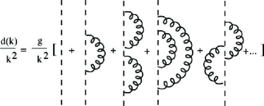
Figure 1: Diagrammatic representation of the expansion of the functional integral for the ghost propagator c.f. Eq. (LABEL:EQ_INV_FP_EXPANSION)

It should be noted that $m_{g}$ is a mass parameter introduced by the ansatz wave functional and should not be confused with the QCD scale introduced by renormalization. The latter appears in the renormalized Dyson equation for the ghost dressing function which, as mentioned earlier, can be identified with the running coupling. In principle, $m_{g}=m_{g}(g_{r}(\mu),\mu)$ should be renormalization point invariant and just like $g_{r}(\mu)$ determined by a physical observable e.g. the string tension. Within the set of truncations build in the derivation of the Dyson series, most likely the renormalization group invariance of $m_{g}$ can not be proven and we shall consider $m_{g}$ as a free parameter. Given $\omega(k)$ the Dyson series for the ghost dressing function can be sum up and represented as a single integral equation within the rainbow-ladder approximation, illustrated in Fig. 1. All omitted diagrams have at least one vertex loop correction (e.g. last diagram in Fig. 1), which were shown to be generally smaller than the self-energy loops Szczepaniak and Swanson (2002). The diagrams shown in Fig. 1 represent functional integrals over $|\Psi[A]|^{2}$ of polynomials of the $A$ field originating from the expansion of the inverse Faddeev-Popov operator

$${1\over{\langle\Psi|\Psi\rangle}}\int_{\Omega}{\cal D}Ag{{g|\Psi[A]|^{2}}\over{-\bm{\nabla}\cdot{\bf D}[A]}}\to$$

$$\to {g\over{-\bm{\nabla}^{2}}}\left[1+{1\over{\langle|\Psi|\Psi\rangle}}\int_{\Omega}{\cal D}Ag{\bf A}\times{{\bm{\nabla}}\over{\bm{\nabla}^{2}}}g{\bf A}\times{{\bm{\nabla}}\over{\bm{\nabla}^{2}}}+\cdots\right]$$

where $\times$ refers to the color space. Neglecting the restriction to the Gribov region enables one to perform the functional integrals analytically, and neglecting contractions that corresponds to vertex corrections makes it possible to re-sum the series, resulting in,

$${1\over{d(k)}}={1\over{g(\Lambda)}}-{N_{C}}\int^{\Lambda}{{d{\bf q}}\over{(2\pi)^{3}2\omega(q)}}{{1-(\hat{\bf k}\cdot\hat{\bf q})^{2}}\over{({\bf k}-{\bf q})^{2}}}d(|{\bf k}-{\bf q}|).$$ (15)

The dependence of the bare coupling, $g=g(\Lambda)$, and the loop integral on the UV cut-off has been shown explicitly. Instead of using the bare coupling and the UV cutoff as the renormalization point, the equation can be renormalized at a finite momentum scale through subtraction, which also defines the renormalized coupling as $g_{r}(\mu)\equiv d(k=\mu)$

$${1\over{d(k)}}={1\over{d(\mu)}}$$

$$- {N_{C}}\int^{\Lambda}{{d{\bf q}}\over{(2\pi)^{3}}}\left[{{1-(\hat{\bf k}\cdot\hat{\bf q})^{2}}\over{({\bf k}-{\bf q})^{2}}}{{d(|{\bf k}-{\bf q}|)}\over{2\omega(q)}}-(|{\bf k}|\to\mu)\right].$$

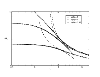
Figure 2: Comparison between the numerical solutions of the Dyson equation for the ghost propagator and the approximate analytical solutions of Eqs. (18), (19). The solid (dashed) lines represent the low (high) momentum behavior, respectively.

As discussed above, the mass scale is brought in through the function $\omega$, and in the case discussed here, it is given by $m_{g}=\omega(0)$. Thus from now on we will use the notation $\tilde{k}\equiv k/m_{g}$ to denote dimensionless momenta. The solution of the Dyson equation for the ghost propagator depends on one more parameter, the value of $d(\tilde{\mu})$ at a single point, i.e. at $\tilde{\mu}=\mu/m_{g}=1$. In Fig. 2 we plot the numerical solutions of Eq. (LABEL:d), as a function of momentum in units of $m_{g}$, for three choices of $d(\tilde{k}=1)$. As $d(1)$ is increased the solutions become more IR enhanced until at, approximately, $d(1)\sim 3.41$ the solution becomes critical Szczepaniak and Swanson (2002). Above this critical point the Dyson equation has no solutions, i.e. develops a Landau point at physical, $k>0$ momentum. This is a sign that the functional integration in Eq. (LABEL:EQ_INV_FP_EXPANSION) has crossed the Gribov horizon. The mass scale dependence of the ghost propagator can be best understood by using an angular approximation, to the integral in Eq. (LABEL:d),

$$|{\bf k}-{\bf q}|\to\theta(k-q)k+\theta(q-k)q,$$ (17)

which enables one to transform the integral equation to a first order differential equation that can be solved analytically and further well approximated by Szczepaniak and Swanson (2002),

$$d(\tilde{k}) = \frac{d(\tilde{\mu})}{\left[1+\beta_{L}d^{1/\gamma}(\tilde{\mu})\left(\tilde{k}-\tilde{\mu}\right)\right]^{\gamma}},~{}\tilde{k}\leq 1,$$ (18)

$$d(\tilde{k}) = \frac{d(\tilde{\mu})}{\left[1+\beta_{H}d^{1/\gamma}(\tilde{\mu})\log\left(\frac{\tilde{k}}{\tilde{\mu}}\right)\right]^{\gamma}},~{}\tilde{k}\geq 1,$$ (19)

where $\gamma=1/2$ and $\beta_{L}=(5/6)(N_{C}/3)/\pi^{2}$ and $\beta_{H}=(N_{C}/3)/\pi^{2}$ i.e. $\beta_{L}\sim\beta_{H}\sim 0.1$ for $N_{C}=3$. It clearly follows that the ghost propagator is independent of the renormalization scale, $\mu$ and depends on a single value of $d(\tilde{\mu})$ at an arbitrarily chosen renormalization point. Furthermore, from Eq. (18) it follows that a solution exists, i.e there is no Landau pole, as long as $d(\tilde{\mu})<1/(\beta_{L}\tilde{\mu})^{\gamma}$.

As discussed above, the approximations leading to Eq. (LABEL:d) include eliminating all vertex corrections and neglecting the restriction on the functional integral to be contained within the Gribov horizon. In the following we present results from a Monte Carlo simulation of the ghost propagator that does not have these limitations.

III Monte Carlo Calculation

The evaluation of the functional integral in Eq. (10) is usually performed analytically by expanding the operator $\mathcal{O}$ in a power series over the gauge field $A$ and truncating at some order (c.f. Eq. (LABEL:EQ_INV_FP_EXPANSION) ). Here we avoid these approximations by evaluating the functional integral by Monte Carlo integration using the model wavefunction (12) with the approximate solution (13) for $\omega(k)$.

The gluon configurations are generated on a $N_{d}=3$ dimensional momentum space grid. The gluon fields $A_{i}^{c}(k)$ are $N_{d}\times(N_{C}^{2}-1)$ complex numbers per lattice site, where $A_{i}^{a}(-k)={A_{i}^{a}}^{\ast}(k)$. The momentum is discretized on the lattice as

$$k_{i}=\frac{2\pi n_{i}}{aN_{i}}\quad\left|n_{i}\right.\quad\in\left(-\frac{N_{i}}{2},\frac{N_{i}}{2}\right],$$ (20)

$$i\in\{1,2,3\},$$ (21)

where $a$ denotes the lattice spacing. The gauge fields must satisfy the position space Coulomb gauge condition

$$\sum_{i=1}^{3}A^{a}_{i}(x)-A^{a}_{i}(x-a\hat{\imath})=0,$$ (22)

which translates in the momentum space to

$$\sum_{i=1}^{3}(1-\cos(ak)+i\sin(ak))A^{a}_{i}(ak)=0.$$ (23)

From now on we will use the notation $\hat{A}(\hat{k})\equiv A(ak)/a^{2}$, etc. in reference to dimensionless quantities scaled with the lattice spacing. The coupling is incorporated by generating $g\hat{A}_{i}^{a}(\hat{k})$ rather than $\hat{A}_{i}^{a}(\hat{k})$, which requires substituting $\omega(k)$ with $\omega(k)/g^{2}$ in the model wavefunction. The gluon fields are generated with the distribution

$$|\Psi[A]|^{2}=\exp\left\{-{1\over{N_{L}^{3}}}\sum_{n_{i}}\sum_{i=1}^{N_{d}}\sum_{a=1}^{N_{c}^{2}-1}\hat{A}_{i}^{a}(\hat{k})\hat{A}_{i}^{a}(-\hat{k})\frac{\hat{\omega}(\hat{k})}{g^{2}}\right\}.$$ (24)

This is accomplished by independently generating two of the vector components, $\hat{A}^{a}_{i}$, with a heatbath, then constructing the third component such that the momentum space Coulomb gauge condition, Eq. (23), is satisfied.

The calculation of the Jacobian is akin to the calculation of the quark determinant in lattice QCD and in the present work it is set to one. The Jacobian was included in Ref. Szczepaniak (2004) in a certain truncation scheme. There it was found to lessen the dependence of the Coulomb potential to the choice of coupling.

As a first test we evaluate the gluon propagator,

$$g^{2}\hat{G}(\hat{k})=\frac{1}{N_{L}^{3}}\frac{1}{N_{d}-1}\frac{1}{N_{c}^{2}-1}\langle\sum_{i=1}^{N_{d}-1}\sum_{a=1}^{N^{2}_{C}-1}\hat{A}_{i}^{a}(\hat{k})\hat{A}_{i}^{a}(-\hat{k})\rangle.$$ (25)

The value of $G(k)$ is analytically known to be $G(k)=1/2\omega(k)$. The numerical result, shown in Fig. 3 does indeed agree with the analytical one, where the numerical statistics are improved by taking the $Z_{3}$ average, that is, averaging over the three equivalent directions in momentum space. Since $\hat{k}=\hat{m}_{g}\tilde{k}$ The physical propagator in units of $m_{g}$ is given by

$$m_{g}G(k)=\hat{m}_{g}\hat{G}(\hat{k}).$$ (26)

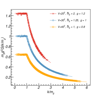
Figure 3: (Color Online) The gluon propagator calculated on $1000$ gauge field configurations with various parameters. The analytic results are plotted as a continuous line, showing a good agreement with simulations.

We now proceed to computing the ghost dressing function. The ghost propagator is expressed as the expectation value of the inverse of the Faddeev-Popov (FP) operator, Eq. (11). The discrete form of the FP operator was derived in Ref. Zwanziger (1994)

$$M^{ab}({\hat{x}},{\hat{y}}){\hat{\phi}}^{b}({\hat{y}})=\sum_{i=1}^{N_{d}}\delta^{ab}\left({\hat{\phi}}^{b}({\hat{y}}+\hat{\imath})+{\hat{\phi}}^{b}({\hat{y}}-\hat{\imath})-2{\hat{\phi}}({\hat{y}})\right)$$

$$-f^{abc}\left({\hat{\phi}}^{b}({\hat{y}}+\hat{\imath}){\hat{A}}_{i}^{c}({\hat{y}})-{\hat{\phi}}^{b}({\hat{y}}-\hat{\imath}){\hat{A}}_{i}^{c}({\hat{y}}-\hat{\imath})\right),$$

which is real and symmetric. Note that the region of integration in Eq. (10) is the Gribov region where $M$ is positive definite. Thus any gauge field configuration that produces a Faddeev-Popov operator with negative eigenvalues must be discarded.

With periodic boundary conditions imposed on the lattice, $M^{ab}(x,y)$ has $N_{c}^{2}-1$ trivial zero modes, making it formally non-invertible. This problem is avoided by following Ref. Boucaud et al. (2005) and solving

$$\int_{V}d{\bf y}M^{ab}({\bf x},{\bf y}){\phi}^{b}({\bf y})=\delta^{ab}\left(\delta({\bf x})-\frac{1}{V}\right).$$ (27)

The position-color vectors are then Fourier transformed to momentum space and the inverse of $M^{ab}(x,0)$ recovered.

$$\int_{V}d{\bf x}e^{-i\mathbf{k}\cdot\mathbf{x}}\left\langle\phi^{a}(x)\right\rangle=\int_{V}d{\bf x}e^{-i{\mathbf{k}\cdot\mathbf{x}}}\left\langle(M^{-1})^{aa}({\bf x},{\bf 0})\right\rangle-\frac{1}{V}\int_{V}d{\bf x}d{\bf y}e^{-i{\mathbf{k}\cdot\mathbf{x}}}\left\langle(M^{-1})^{aa}({\bf x},{\bf y})\right\rangle={{D(k)}\over g}-\delta({\bf k})\int_{V}d{\bf x}{{D(x)}\over g},$$ (28)

where $D(k)\equiv d(k)/k^{2}$. The average is taken over gauge field configurations, and finally the ghost propagator is $Z_{3}$ averaged. In the free case, $M\rightarrow-\nabla^{2}$ and the propagator would be

$$\hat{D}(\hat{k})=\frac{g}{4\sum_{i}\sin^{2}(\hat{k}_{i}/2)}\equiv\frac{g}{k^{2}},\\$$ (29)

which defines an appropriate momentum variable. The same philosophy is used in conventional lattice QCD studies of gluon propagator Bonnet et al. (2001); Leinweber et al. (1998); Marenzoni et al. (1995).

With the model wavefunction (12), the coupling $g$ is a free parameter. The larger $g$ is chosen to be, the broader the Gaussian. This increases the fluctuations of the gauge fields and $M$ develops smaller eigenvalues, resulting in the infrared enhancement of $\left\langle M^{-1}(k)\right\rangle$. With increasing the value of $g$, the FP operator becomes likely to develop negative eigenvalues. While this means that a (possibly large) proportion of the generated gauge fields must be rejected, it is necessary for the entire domain of the functional integration to be sampled. The number of rejected configurations grows rapidly when the value of $g$ approaches certain critical value, which depends on the value of $m_{g}$ used in the model for $\omega(k)$ of Eq. (13). This is easily understandable, as larger value of $m_{g}$ means the gluon wavefunction is infrared enhanced in a larger interval of momenta, yielding narrower Gaussian width over that interval.

Each generated gauge configuration used in calculating the ghost dressing function is checked to lay in the Gribov region by calculating several eigenvalues of the FP operator to ensure their positivity. If the latter constrain is not imposed, the resulting ghost propagators are dominated by numerical fluctuations (resemble random noise) in the region where the generated gauge configurations have large fraction laying outside of Gribov region. For example, for $\hat{m}_{g}=1.5$, the fraction of rejected configuration ranges from nearly $0\%$ for $g<1$ to $100\%$ for $g>1.1$ with sharp increase above $g=1$. For $\hat{m}_{g}=5$ this “critical” value of $g$ increases to about $1.6$ . In our calculations we restrict to the region of $g$, where the fraction of rejected configurations does not exceed $20\%$ to maintain moderate computational time. The resulting ghost dressing function is shown in Fig. 4 for a calculation with $1000$ gluon configurations on a $40^{3}$ lattice with $\hat{m}_{g}=1.25$ and $g=0.7$.

In order to relate the calculated ghost dressing function to the physical region several issues should be resolved that would allow to draw a correspondence. Here we review the most relevant ones.

III.1 Lattice Artifacts

Discretization of space introduces several artifacts, that should be accounted for. These are errors introduced by finite lattice volume, finite lattice spacing, which also induces broken spatial rotational symmetry.

III.1.1 Finite Lattice Spacing

It is argued in the Refs. Bonnet et al. (2001); Leinweber et al. (1998); Marenzoni et al. (1995) that using the redefined lattice momentum variable of Eq. (29) allows one to avoid the leading-order discretization errors arising from the ultra-violet cutoff in momentum introduced by the finite lattice spacing. Still, the errors from reducing the spatial rotational symmetry $O(3)$ group down to discrete $Z(3)$ are unaccounted for. These manifest themselves as a large spread in the ghost propagator. This spread occurs in a characteristic pattern, as can be seen in Fig. 4, which becomes more prominent with increased lattice volume. These patterns can be easily understood by considering a selection of subsets of the points plotted by using certain criteria imposed on the momentum variable. The first subset considered has the constraint that all three components of the momentum are equal to each other (laying on the diagonal direction of the lattice). This selection of the data forms a smooth line through the upper part of the plot. A subset including points with two of the momentum components equal to each other and the third one set to zero (along the diagonal direction of the cube’s side) forms another smooth curve, this one going through the middle of the plot. Finally, the subset with only one non-zero component of momentum (along the side of the cube) forms a line passing through the lowest part of the plot. These subsets are shown in Fig. 5a. Furthermore, if the constraints described above are allowed to be violated by a few units of minimum lattice momentum, the rest of the points in the plot start to fall into these subgroups, as shown in Fig. 5b. Thus, for the further analysis of our data we will use only a subset of points with momentum components not differing from each other by more than one unit of minimum lattice momentum. This is the “cylinder cut” introduced in Refs. Leinweber et al. (1998); Bonnet et al. (2001), which allows us to select the points least affected by errors introduced by the broken rotational symmetry and leaves a sufficient number of points for statistical analysis.

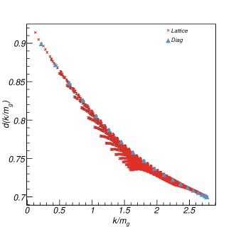
Figure 4: (Color Online) Ghost dressing function $d(k/m_{g})$ versus $k/m_{g}$ for $\hat{m}_{g}=1.25$ and $g=0.7$ on a lattice with $40^{3}$ volume. Here the crosses denote the full data set and open triangles denote the subset of points with equal momenta components.

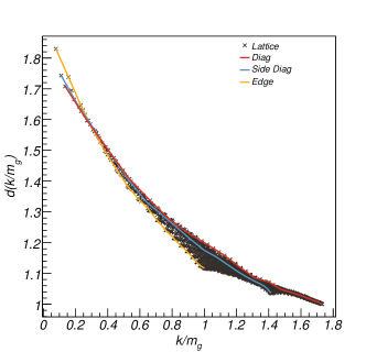
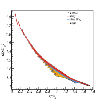
Figure 5: (Color Online) Ghost dressing function for $d(k/m_{g})$ versus $k/m_{g}$ for $\hat{m}_{g}=1.25$ and $g=0.7$ on a lattice with $40^{3}$ volume. Here the crosses denote the data points and the three lines connect the subsets of the points laying within $0$ a) and $7$ b) minimum lattice momenta correspondingly of the edge, the side diagonal and the diagonal directions of the momentum lattice cube.

III.1.2 Finite Volume Effects

While a consistent treatment of the finite volume effects requires extensive investigation into discretization of the theory on the lattice, here we simply investigate this dependence by comparing benchmark calculations on lattices with different volumes. A set of calculations with four different lattice volumes is shown in Fig. 6, which shows that there are very small variations only in the low momenta region for lattice volumes from $20^{3}$ to $40^{3}$. Thus we choose to use lattice volume of $20^{3}$ for the further calculations, which allows for both reasonable computational time and small errors.

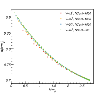
Figure 6: (Color Online) Ghost dressing function $d(k/m_{g})$ versus $k/m_{g}$ for $\hat{m}_{g}=1.25$ and $g=0.7$. We show the influence of varying the lattice volume $V$ on the calculated data points with momentum components not differing by more than two units lattice momentum, as described in the text. Here $NConf$ denotes the number of the sampled gluon configurations.

III.2 Renormalization

The introduction of a finite momentum grid provides a sharp cutoff for the regularization of the ultra-violet divergences, i.e. it is equivalent to the role of $\Lambda$ in Eq. (15). In order to identify the ghost dressing function with the running coupling, for each lattice spacing it should be possible to choose the lattice coupling, $g$ in Eq. (24), so that the results of simulations are independent of the lattice spacing. In the simulation, explicit dependence on the lattice spacing enters through dependence on $\hat{m}_{g}=am_{g}$, e.g. when the lattice ghost dressing function is plotted against $\tilde{k}=k/m_{g}=\hat{k}/\hat{m}_{g}$ the result should be independent of $\hat{m}_{g}$ and depend only on the value of the renormalized coupling. In practice, we produce a series of simulations with different values of $g$ in the range between $g=0.5-1.5$ and $\hat{m}_{g}$ in the range of the accessible lattice momenta $2\pi/N_{Lat}\leq\hat{m}_{g}\leq\sqrt{3}\pi$. We then compare with the scaling predicted by the solutions of the Dyson equations given in Eqs. (18) and (19), in the low and high momentum region, respectively. In the high momentum regime, $k/m_{g}=\hat{k}/\hat{m}_{g}$ is kept large by running simulations with small $\hat{m}_{g}$ i.e. with $\hat{m}_{g}\gtrsim 2\pi/N_{Lat}$. In this regime the constituent gluon mass is close to the minimum accessible momentum scale on the lattice and the gluon propagator is close to asymptotic while the non-perturbative effects are only present for a few, lowest momentum points. This regime should be described by Eq. (19),

$$d(\tilde{k})=\frac{d(\tilde{\mu})}{\left[1+\beta^{\prime}_{H}d^{1/\gamma^{\prime}}(\tilde{\mu})\log\left(\frac{\tilde{k}}{\tilde{\mu}}\right)\right]^{\gamma^{\prime}}},$$ (30)

where $\beta^{\prime}_{H}$ and $\gamma^{\prime}$ will be treated as fit parameters. For $N_{d}=20$ each data set has $30$ momentum points after the imposed “diagonal” cut described above. We choose $6$ data sets with $\hat{m}_{g}\in[0.1,1]$ and $g\in[0.3,0.75]$, where the $25$ highest momentum points can be considered to be in the asymptotic region. For each value of the coupling, $g$, the value of $d(\tilde{\mu})$ is fixed by the data itself with $\tilde{\mu}$ set equal to the momentum cut-off, $\tilde{\mu}=\sqrt{3}\pi/\hat{m}_{g}$. The formula in Eq. (19) is fitted to all $150$ data points by varying $\beta^{\prime}_{H}$ and $\gamma^{\prime}$. The resulting remarkably good fits are shown in Fig. 7 with the best-fit value of $\beta^{\prime}_{H}=0.86(2)$ and $\gamma^{\prime}=0.5(2)$. The data deviate from the perturbative form at intermediate momenta, which is to be expected.

On the other hand, in simulations with large $\hat{m}_{g}$ i.e for $\hat{m}_{g}\lesssim\sqrt{3}\pi$, Eq. (18) should apply. Then the constituent gluon mass is close to the largest accessible momentum scale on the lattice. This regime is dominated by non-propagating gluons induced by non-perturbative dressing. Here we expect,

$$d(\tilde{k})=\frac{d(\tilde{\mu})}{\left[1+\beta^{\prime}_{L}d^{1/\gamma^{\prime}}(\tilde{\mu})\left(\tilde{k}-\tilde{\mu}\right)\right]^{\gamma^{\prime}}}.$$ (31)

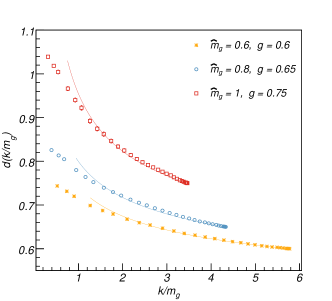
Figure 7: (Color Online) Simultaneous fits to the ghost dressing function $d(k/m_{g})$ versus $k/m_{g}$ for $\hat{m}_{g}\gtrsim 2\pi/N_{Lat}$.

In this region we select a total of $8$ data sets composed of $\hat{m}_{g}\in[3,5]$ and $g\in[1,1.4]$, where the $15$ lowest momentum points can be considered to be in the non-perturbative region. Here, $d(\tilde{\mu})$ is obtained from each data set itself, at $\tilde{\mu}$ chosen, to avoid finite-volume effects, to be the second lowest momentum point. In the low momentum range a total of $120$ data points was fitted varying $\beta^{\prime}_{L}$ while keeping $\gamma^{\prime}=1/2$ which was previously determined from the high momentum fit. A sample of data points with the corresponding fits are shown in Fig. 8 for the best fit value of $\beta^{\prime}_{L}=0.81(2)$. Again, the discrepancies in the higher momentum region are expected as a consequence of deviations from purely non-perturbative behavior set by the asymptotic tail of the gluon propagator.

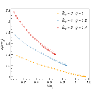
Figure 8: (Color Online) Simultaneous fits to the ghost dressing function $d(k/m_{g})$ versus $k/m_{g}$ for $\hat{m}_{g}\lesssim\sqrt{3}\pi$.

IV Conclusions

We have computed the ghost correlation function by direct Monte Carlo simulation of the functional integral with a model gaussian wave functional and compared it with the solution of the corresponding Dyson equation. We have found that the scaling behavior of the solution of the Dyson equation is reproduced in the simulation. This confirms that the corrections to the rainbow-ladder approximation are both IR and UV finite, and do not change the scaling properties. The $\beta$ function obtained from simulations is, however, an order of magnitude larger than the one from the Dyson equation. This is to be expected, since the Dyson equation does not properly take into account the boundary of the field space integral, and thus is expected to overestimate the magnitude of the allowed field values and thus of the critical coupling. The Monte Carlo simulation still needs to have the Faddeev-Popov Jacobian implemented, but that is not expected to qualitatively change the results.

In our simulations we have found that positivity of the Faddeev-Popov operator is not sufficient to produce critical behavior. This needs to be investigated further, in particular on larger volumes; nevertheless, since the simple gaussian vacuum wave functional does not probe topological configurations (e.g. of magnetic disorder) it is not too surprising that the IR enhancement of the ghost correlator or Coulomb form factor fails to quantitatively reproduce confinement. For this purpose a wave functional of the type proposed in Ref. Greensite and Olejnik (2008) should be tried.

V Acknowledgment

We would like to thank H. Reinhardt for continuing discussions of the Coulomb gauge QCD. This work was supported in part by the US Department of Energy grant under contract DE-FG0287ER40365.

References

- Natale (2007) A. A. Natale, Braz. J. Phys. 37, 306 (2007), eprint hep-ph/0610256.
- Fischer (2006) C. S. Fischer, J. Phys. G32, R253 (2006), eprint hep-ph/0605173.
- von Smekal et al. (1998) L. von Smekal, A. Hauck, and R. Alkofer, Ann. Phys. 267, 1 (1998), eprint hep-ph/9707327.
- Braun et al. (2007) J. Braun, H. Gies, and J. M. Pawlowski (2007), eprint 0708.2413.
- Zwanziger (2002) D. Zwanziger, Phys. Rev. D65, 094039 (2002), eprint hep-th/0109224.
- Pawlowski et al. (2004) J. M. Pawlowski, D. F. Litim, S. Nedelko, and L. von Smekal, Phys. Rev. Lett. 93, 152002 (2004), eprint hep-th/0312324.
- Lerche and von Smekal (2002) C. Lerche and L. von Smekal, Phys. Rev. D65, 125006 (2002), eprint hep-ph/0202194.
- Aguilar and Natale (2004) A. C. Aguilar and A. A. Natale, JHEP 08, 057 (2004), eprint hep-ph/0408254.
- Frasca (2007) M. Frasca (2007), eprint 0709.2042.
- Boucaud et al. (2007a) P. Boucaud et al., Eur. Phys. J. A31, 750 (2007a), eprint hep-ph/0701114.
- Boucaud et al. (2007b) P. Boucaud et al., JHEP 03, 076 (2007b), eprint hep-ph/0702092.
- Chernodub and Zakharov (2007) M. N. Chernodub and V. I. Zakharov (2007), eprint hep-ph/0703167.
- Dudal et al. (2007) D. Dudal, S. P. Sorella, N. Vandersickel, and H. Verschelde (2007), eprint 0711.4496.
- Cucchieri (1997) A. Cucchieri, Nucl. Phys. B508, 353 (1997), eprint hep-lat/9705005.
- Ilgenfritz et al. (2007) E. M. Ilgenfritz, M. Muller-Preussker, A. Sternbeck, A. Schiller, and I. L. Bogolubsky, Braz. J. Phys. 37, 193 (2007), eprint hep-lat/0609043.
- Leinweber et al. (1998) D. B. Leinweber, J. I. Skullerud, A. G. Williams, and C. Parrinello (UKQCD), Phys. Rev. D58, 031501 (1998), eprint hep-lat/9803015.
- Furui and Nakajima (2004) S. Furui and H. Nakajima, Phys. Rev. D69, 074505 (2004), eprint hep-lat/0305010.
- Cucchieri and Mendes (2007a) A. Cucchieri and T. Mendes, Braz. J. Phys. 37, 484 (2007a), eprint hep-ph/0605224.
- Cucchieri (1999) A. Cucchieri, Phys. Rev. D60, 034508 (1999), eprint hep-lat/9902023.
- Cucchieri et al. (2003) A. Cucchieri, T. Mendes, and A. R. Taurines, Phys. Rev. D67, 091502 (2003), eprint hep-lat/0302022.
- Sternbeck et al. (2005) A. Sternbeck, E. M. Ilgenfritz, M. Mueller-Preussker, and A. Schiller, Phys. Rev. D72, 014507 (2005), eprint hep-lat/0506007.
- Boucaud et al. (2005) P. Boucaud et al., Phys. Rev. D72, 114503 (2005), eprint hep-lat/0506031.
- Bogolubsky et al. (2006) I. L. Bogolubsky, G. Burgio, M. Muller-Preussker, and V. K. Mitrjushkin, Phys. Rev. D74, 034503 (2006), eprint hep-lat/0511056.
- Cucchieri et al. (2006) A. Cucchieri, A. Maas, and T. Mendes, Phys. Rev. D74, 014503 (2006), eprint hep-lat/0605011.
- Oliveira and Silva (2007a) O. Oliveira and P. J. Silva, Braz. J. Phys. 37, 201 (2007a), eprint hep-lat/0609036.
- Oliveira and Silva (2007b) O. Oliveira and P. J. Silva, Eur. Phys. J. A31, 790 (2007b), eprint hep-lat/0609027.
- Fischer et al. (2002) C. S. Fischer, R. Alkofer, and H. Reinhardt, Phys. Rev. D65, 094008 (2002), eprint hep-ph/0202195.
- Fischer et al. (2006) C. S. Fischer, B. Gruter, and R. Alkofer, Ann. Phys. 321, 1918 (2006), eprint hep-ph/0506053.
- Fischer et al. (2007a) C. S. Fischer, A. Maas, J. M. Pawlowski, and L. von Smekal, Annals Phys. 322, 2916 (2007a), eprint hep-ph/0701050.
- Fischer et al. (2007b) C. S. Fischer, R. Alkofer, A. Maas, J. M. Pawlowski, and L. von Smekal, POS LAT2007, 300 (2007b), eprint 0709.3205.
- Cucchieri and Mendes (2007b) A. Cucchieri and T. Mendes (2007b), eprint 0710.0412.
- Bogolubsky et al. (2007) I. L. Bogolubsky, E. M. Ilgenfritz, M. Muller-Preussker, and A. Sternbeck (2007), eprint 0710.1968.
- Sternbeck et al. (2007) A. Sternbeck, L. von Smekal, D. B. Leinweber, and A. G. Williams (2007), eprint 0710.1982.
- Cucchieri et al. (2007) A. Cucchieri, T. Mendes, O. Oliveira, and P. J. Silva, Phys. Rev. D76, 114507 (2007), eprint 0705.3367.
- Cucchieri and Mendes (2007c) A. Cucchieri and T. Mendes (2007c), eprint 0712.3517.
- Bowman et al. (2007) P. O. Bowman et al., Phys. Rev. D76, 094505 (2007), eprint hep-lat/0703022.
- Kugo and Ojima (1979) T. Kugo and I. Ojima, Prog. Theor. Phys. Suppl. 66, 1 (1979).
- Kugo (1995) T. Kugo (1995), eprint hep-th/9511033.
- Caudy and Greensite (2007) W. Caudy and J. Greensite (2007), eprint 0712.0999.
- Zwanziger (2003) D. Zwanziger, Phys. Rev. Lett. 90, 102001 (2003), eprint hep-lat/0209105.
- Zwanziger (1997) D. Zwanziger, Nucl. Phys. B485, 185 (1997), eprint hep-th/9603203.
- Epple et al. (2007a) D. Epple, H. Reinhardt, and W. Schleifenbaum, Phys. Rev. D75, 045011 (2007a), eprint hep-th/0612241.
- Cucchieri (2007) A. Cucchieri, AIP Conf. Proc. 892, 22 (2007), eprint hep-lat/0612004.
- Cucchieri and Zwanziger (1997) A. Cucchieri and D. Zwanziger, Phys. Rev. Lett. 78, 3814 (1997), eprint hep-th/9607224.
- Epple et al. (2007b) D. Epple, H. Reinhardt, W. Schleifenbaum, and A. P. Szczepaniak (2007b), eprint 0712.3694.
- Gribov (1978) V. N. Gribov, Nucl. Phys. B139, 1 (1978).
- Zwanziger (1994) D. Zwanziger, Nucl. Phys. B412, 657 (1994).
- Dokshitzer and Kharzeev (2004) Y. L. Dokshitzer and D. E. Kharzeev, Ann. Rev. Nucl. Part. Sci. 54, 487 (2004), eprint hep-ph/0404216.
- Zwanziger (1991a) D. Zwanziger, Phys. Lett. B257, 168 (1991a).
- Zwanziger (1991b) D. Zwanziger, Nucl. Phys. B364, 127 (1991b).
- Szczepaniak and Swanson (2002) A. P. Szczepaniak and E. S. Swanson, Phys. Rev. D65, 025012 (2002), eprint hep-ph/0107078.
- Szczepaniak (2004) A. P. Szczepaniak, Phys. Rev. D69, 074031 (2004), eprint hep-ph/0306030.
- Feuchter and Reinhardt (2004a) C. Feuchter and H. Reinhardt, Phys. Rev. D70, 105021 (2004a), eprint hep-th/0408236.
- Feuchter and Reinhardt (2004b) C. Feuchter and H. Reinhardt (2004b), eprint hep-th/0402106.
- Reinhardt and Feuchter (2005) H. Reinhardt and C. Feuchter, Phys. Rev. D71, 105002 (2005), eprint hep-th/0408237.
- Christ and Lee (1980) N. H. Christ and T. D. Lee, Phys. Rev. D22, 939 (1980).
- Zwanziger (2004) D. Zwanziger, Phys. Rev. D69, 016002 (2004), eprint hep-ph/0303028.
- Swift (1988) A. R. Swift, Phys. Rev. D38, 668 (1988).
- Bonnet et al. (2001) F. D. R. Bonnet, P. O. Bowman, D. B. Leinweber, A. G. Williams, and J. M. Zanotti, Phys. Rev. D64, 034501 (2001), eprint hep-lat/0101013.
- Marenzoni et al. (1995) P. Marenzoni, G. Martinelli, and N. Stella, Nucl. Phys. B455, 339 (1995), eprint hep-lat/9410011.
- Greensite and Olejnik (2008) J. Greensite and S. Olejnik, Phys. Rev. D77, 065003 (2008), eprint arXiv:0707.2860.