Sub-Alfv$\acute{\rm e}$nic Non-Ideal MHD Turbulence Simulations with Ambipolar Diffusion: I. Turbulence Statistics

Abstract

Most numerical investigations on the role of magnetic fields in turbulent molecular clouds (MCs) are based on ideal magneto-hydrodynamics (MHD). However, MCs are weakly ionized, so that the time scale required for the magnetic field to diffuse through the neutral component of the plasma by ambipolar diffusion (AD) can be comparable to the dynamical time scale. We have performed a series of $256^{3}$ and $512^{3}$ simulations on supersonic but sub-Alfv$\acute{\rm e}$nic turbulent systems with AD using the Heavy-Ion Approximation developed in Li et al. (2006). Our calculations are based on the assumption that the number of ions is conserved, but we show that these results approximately apply to the case of time-dependent ionization in molecular clouds as well. Convergence studies allow us to determine the optimal value of the ionization mass fraction when using the heavy-ion approximation for low Mach number, sub-Alfv$\acute{\rm e}$nic turbulent systems. We find that ambipolar diffusion steepens the velocity and magnetic power spectra compared to the ideal MHD case. Changes in the density PDF, total magnetic energy, and ionization fraction are determined as a function of the AD Reynolds number. The power spectra for the neutral gas properties of a strongly magnetized medium with a low AD Reynolds number are similar to those for a weakly magnetized medium; in particular, the power spectrum of the neutral velocity is close to that for Burgers turbulence.

1 Introduction

Both supersonic turbulence and magnetic fields are widely observed in molecular clouds (MCs). MCs have broad line widths, ranging from a few to more than 10 times the sound speed, $c_{s}$ (Elmegreen & Scalo, 2004). The observed interstellar magnetic field strength is a few micro Gauss (e.g. Heiles & Troland, 2005), in rough equipartition with the kinetic energy in the interstellar medium. If the magnetic field were perfectly frozen into the interstellar gas during the gravitational collapse of a protostar, the magnetic field strength of a typical star like our Sun would be more than 10 orders of magnitude larger than we observe today. Thus there must be some mechanisms that are effective in removing the excess magnetic flux during the star formation process. Mestel & Spitzer (1956) first suggested that ambipolar diffusion (AD) could allow magnetic flux to be redistributed during collapse in low ionization regions in MCs as the result of the differential motion between the ionized and neutral gas. Since then, much work has been done on AD-driven collapse of MCs (e.g. Spitzer, 1968; Nakano & Tademaru, 1972; Mouschovias, 1976, 1977, 1979; Nakano & Nakamura, 1978; Shu, 1983; Lizano & Shu, 1989; Fiedler & Mouschovias, 1992, 1993).

AD-driven gravitational contraction is a quasi-static process. The AD timescale, $t_{\rm AD}$, in a typical MC is about ten times the free-fall time, $t_{\rm ff}$ (McKee & Ostriker, 2007). Once AD has removed a sufficient amount of magnetic flux, a thermally supported core with a mass in excess of the Bonnor-Ebert mass will collapse in about a free-fall time. However, MCs are observed to be supersonically turbulent. Numerical simulations have shown that turbulence is an efficient mechanism for supporting MCs globally, while at the same time providing seeds for gravitational collapse by shock compression. (e.g. Klessen et al., 2000; Heitsch et al., 2001; Li et al., 2004). By driving large fluctuations in the density, velocity and magnetic field, turbulence significantly reduces the AD timescale (Fatuzzo & Adams, 2002; Zweibel, 2002). AD significantly redistributes magnetic flux. While the importance of this process has long been recognized in studies of star formation, it is also important in the simpler case in which self-gravity is weak. We therefore wish to determine how AD affects the properties of supersonic, magnetized turbulence such as that inferred in MCs.

It is very challenging to carry out three-dimensional (3D) simulations of AD in molecular clouds. The small ionization fraction in molecular clouds means that the ion inertia can be neglected. If the AD is treated as diffusion of the magnetic field in a single fluid, the time step in explicit codes scales as the square of the grid-size ($\Delta x^{2}$), which is prohibitive at high resolution; the time step is also proportional to the ionization, making it impossible to simulate the small ionizations found in MCs (Mac Low et al., 1995). Treating the ions and neutrals separately as two fluids permits a time step proportional to $\Delta x$, but the necessity of following the Alfv$\acute{\rm e}$n waves in the ion fluid again leads to very small time steps. Two-dimensional fully-implicit codes (e.g. Fiedler & Mouschovias, 1992) were developed to avoid this problem, but complex code development would be required to extend this to three dimensions. In addition, implicit treatments can involve multiple iterations to converge, which may offset the advantage from the larger timestep. Some attempts have been made to perform 3D turbulence simulations with AD with semi-implicit schemes (e.g. Mac Low & Smith, 1997; Falle, 2003) but with a heavy cost on computational time.

To overcome this problem, we introduced the heavy-ion approximation (Li et al., 2006), in which the ionization mass fraction is increased (so as to reduce the ion Alfv$\acute{\rm e}$n velocity) and the ion-neutral collisional coupling constant decreased, with the combined result that the ion-neutral drag is unchanged. With this approximation, one can perform non-ideal MHD turbulence simulations using a two-fluid approach while retaining an accurate treatment of the dynamical interaction between the ions and neutrals in systems with realistic ionization fractions. Oishi & Mac Low (2006) independently made this approximation and used it to make a preliminary study of turbulence with AD. Li et al. (2006) discussed the accuracy of the heavy-ion approximation and developed criteria for the use of this approximation in treating MHD flows with AD.

In this paper, we investigate the effects of AD on sub-Alfv$\acute{\rm e}$nic turbulent flows with a series of $256^{3}$ and $512^{3}$ MHD turbulence simulations using ZEUS-MPAD (see Li et al. 2006) with the heavy-ion approximation. The AD Reynolds number, $R_{\rm AD}$, is an important metric in the determination of the significance of AD on turbulent flow (Zweibel & Brandenburg, 1997; Li et al. 2006)—for $R_{\rm AD}\gg 1$, the flow is approximately an ideal MHD flow, whereas for $R_{\rm AD}\ll 1$ the flow of the neutrals approaches a purely hydrodynamic flow. We wish to determine the effect of varying the AD Reynolds number on turbulence: How do the statistical properties of a turbulent flow depend upon the AD Reynolds number as the flow changes from the strong ideal MHD case to the strong AD case? How do the effects of turbulent driving of both the neutral and ion gas differ from driving of the neutral component alone? What are the criteria necessary to achieve convergence in both the spatial domain and in the simulation-time domain when using the heavy-ion approximation? What value of the ionization fraction can be used in this approximation and what errors are obtained as a function of the ionization fraction used? What is the effect of AD on the velocity and the magnetic field power spectra? How do these power spectra compare with recent theoretical work on incompressible turbulence in a strong magnetic field? How do the power spectral indices compare with more classical turbulent models for smooth, incompressible flows and shocked, compressible flows? It is well known that the probability density function (PDF) for the density in supersonic isothermal turbulence is log-normal. Is this behavior valid in the presence of AD? Finally, how does the presence of ambipolar diffusion in strongly magnetized turbulent clouds affect our interpretation of the observed power spectra from these clouds?

We discuss the heavy-ion approximation and the requirements for its validity in §2. In §3, we describe our models based on dimensionless model parameters. Because of the size of the parameter space of non-ideal MHD supersonic turbulence, we focus our work on sub-Alfv$\acute{\rm e}$nic turbulence with a thermal Mach number ${\cal M}$ = 3. In §4, we report our convergence study with the heavy-ion approximation, investigating both spatial and temporal convergence. In §5, we report the results on the power spectra of ion and neutral velocities and of the magnetic field in turbulence as a function of $R_{\rm AD}$. In §6, we discuss the probability density function (PDF) of the gas density in the turbulent system. In §7, we investigate other physical properties of the turbulent systems that scale with $R_{\rm AD}$. We summarize our results in §8. Most of the models investigated in details in this paper are based on the assumption of ion conservation. However, high density MCs generally have an ionization equilibrium timescale that is shorter than the dynamical timescale, so that the ionization inside MCs is most likely close to equilibrium. In the Appendix, we demonstrate that nonetheless the assumption of ion conservation is generally a satisfactory approximation for molecular clouds. The astrophysical implications of our turbulence simulations will be reported in a subsequent paper.

2 The Heavy-Ion Approximation

In paper I, we formulated the heavy-ion approximation method for a two-fluid approach to MHD simulations with AD. The isothermal MHD equations for the two fluids, ions and neutrals, with AD are:

$$\frac{\partial\rho_{n}}{\partial t} = -{\bf\nabla}\cdot(\rho_{n}{\bf v}_{n}),$$ (1)

$$\frac{\partial\rho_{i}}{\partial t} = -{\bf\nabla}\cdot(\rho_{i}{\bf v}_{i}),$$ (2)

$$\rho_{n}\frac{\partial{\bf v}_{n}}{\partial t} = -\rho_{n}({\bf v}_{n}\cdot{\bf\nabla}){\bf v}_{n}-{\bf\nabla}P_{n}-{\gamma_{\rm AD}}\rho_{i}\rho_{n}({\bf v}_{n}-{\bf v}_{i}),$$ (3)

$$\rho_{i}\frac{\partial{\bf v}_{i}}{\partial t} = -\rho_{i}({\bf v}_{i}\cdot{\bf\nabla}){\bf v}_{i}-{\bf\nabla}P_{i}-{\gamma_{\rm AD}}\rho_{i}\rho_{n}({\bf v}_{i}-{\bf v}_{n})+\frac{1}{4\pi}\left({\bf\nabla\times}{\bf B}\right){\bf\times}{\bf B},$$ (4)

$$\frac{\partial{\bf B}}{\partial t} = {\bf\nabla\times}({\bf v}_{i}{\bf\times}{\bf B}),$$ (5)

$${\bf\nabla}\cdot{\bf B} = 0,$$ (6)

where $\rho$ = density, v= velocity, B= magnetic field strength, and ${\gamma_{\rm AD}}$ = ion-neutral collisional coupling constant (note that in Paper I, this was denoted as $\gamma$). The subscripts $i$ and $n$ denote ions and neutrals, respectively. Note that in this paper we do not include gravity, so the gravitational terms in the two momentum equations have been omitted. In writing these equations, we have assumed that ions and neutrals are conserved, as in Paper I. This is accurate only if the flow time is small compared to the recombination time. The inclusion of time-dependent chemistry brings in a number of uncertainties (Dalgarno, 2006). However, as we show in the Appendix, the contribution from the ionization source terms is in general small compared to the AD drag term and can be ignored.

We define the ionization mass fraction as

$$\chi_{i}\equiv\frac{\rho_{i}}{\rho_{n}},$$ (7)

which we assume to be small. For $\chi_{i}\ll 1$, as is the case in molecular clouds, we could equally well define $\chi_{i}$ as the ratio of $\rho_{i}$ to the total density $\rho$, but in some of our numerical models we consider values of $\chi_{i}$ as large as 0.1, so that $\rho_{n}$ and $\rho$ are not equivalent. For simplicity, we set the physical value of the ionization mass fraction at a typical observed value of $\chi_{i0,\rm\,phys}=10^{-6}$ in our simulations.

In paper I, we followed Mac Low & Smith (1997) in implementing a semi-implicit method for solving the momentum equations (3) and (4) in the ZEUS-MP code. The new code, ZEUS-MPAD, was tested with several standard AD problems in Paper I. For a two-fluid code, the Courant condition restricts the timestep $\Delta t$ to be less than $\Delta x/v_{\rm Ai}\propto\sqrt{\chi_{i}}$, where $v_{\rm Ai}$ is the ion Alfv$\acute{\rm e}$n velocity. For the low ionizations observed in molecular clouds, $\chi_{i}\sim 10^{-6}$, it is still not feasible to perform turbulence simulations even on the latest state-of-the-art supercomputing platforms. This problem is compounded because intermittency and the highly supersonic nature of the turbulence generate very large contrasts in density. For the neutral component, the low density regions could have densities as low as $10^{-4}\rho_{n0}$ (e.g. Li et al., 2004), and the ion density could be even lower. Therefore, we adopt the heavy-ion approximation developed in Paper I, in which the initial ion mass fraction $\chi_{i0}$ is increased but the ion-neutral coupling coefficient ${\gamma_{\rm AD}}$ is decreased so as to maintain the same product ${\gamma_{\rm AD}}\chi_{i}={\gamma_{\rm AD,\,phys}}\chi_{i0,\rm\,phys}.$ Following the convention established in Paper I, we set the physical value of the ion-neutral coupling coefficient ${\gamma_{\rm AD,\,phys}}=9.21\times 10^{13}$ cm³ g^-1 s^-1, so that our simulations have ${\gamma_{\rm AD}}\chi_{i0}=9.21\times 10^{7}$ cm³ g^-1 s^-1. The heavy-ion approximation reduces the frequency of Alfv$\acute{\rm e}$n waves in the ions, which correspondingly increases the integration timestep, but it maintains the same dynamical coupling between ions and neutrals. We performed three tests in Paper I—the formation of a C-shock, the Wardle instability, and a one-dimensional self-gravitating AD collapse—and demonstrated that MHD simulations with AD can be sped up by a factor of 10 to 100, depending on the problem, without seriously affecting the accuracy. In this paper, we shall consider values of $\chi_{i0}$ from $10^{-4}$ to $10^{-1}$—i.e., $10^{2}-10^{5}$ times greater than the typical physical value. We shall show that $\chi_{i0}=10^{-2}$, corresponding to a speed-up by a factor $\sim 100$, gives good accuracy.

The importance of AD to the flow on a length scale $\ell$ is determined by the ambipolar diffusion Reynolds number,

$$R_{\rm AD}(\ell)\equiv\frac{\ell v}{t_{\rm ni}v_{A}^{2}}=\frac{4\pi{\gamma_{\rm AD}}\rho_{i}\rho_{n}\ell v}{{\langle B^{2}\rangle}}=\frac{\ell}{\ell_{\rm AD}};$$ (8)

where $\ell_{\rm AD}$ is the AD length scale (Zweibel & Brandenburg, 1997; Zweibel, 2002) The three tests in Paper I all had $R_{\rm AD}\sim 1$ on the length scale of the problem. Supersonic turbulent flows have large contrasts in density, velocity, and magnetic field, and as a result there is a large range of length scales involved. The length scales of the local magnetic and velocity fields are

$$\ell_{\delta B} = \left|\frac{\delta B}{{\bf\nabla}\delta B}\right|,$$ (9)

$$\ell_{v} = \left|\frac{v}{{\bf\nabla}v}\right|,$$ (10)

where $\delta B$ is the change in magnetic field from the mean field $B$. and where we have assumed that the mean velocity of the system is zero. Since the ion inertia is negligible in the astrophysical problem, it is necessary to ensure that it remains small when the heavy ion approximation is used. By comparing the inertia term and the AD drag term in the momentum equations, we deduced in Paper I that this requires

$$R_{\rm AD}(\ell_{v_{i}})\gg{{\cal M}_{{\rm A}i}}^{2}$$ (11)

where $\ell_{v_{i}}\sim\ell_{\delta B}$. We shall verify that this condition is satisfied in our simulations.

3 Summary of Simulations

In this paper, we present a series of scale-free turbulence simulations with AD. Three dimensionless numbers characterize the simulations: (1) ${\cal M}\equiv 3^{1/2}\sigma_{\rm nt}/c_{s}$, the 3D rms Mach number of the turbulence, where $\sigma_{\rm nt}$ is the 1D rms nonthermal velocity dispersion; (2) the plasma $\beta=8\pi\rho c_{s}^{2}/{\langle B^{2}\rangle}$, which measures the importance of the magnetic field; and (3) $R_{\rm AD}(\ell_{0})$, the AD Reynolds number on the scale of the box, which measures the importance of AD. The relative importance of the magnetic field on the dynamics of the gas as a whole and on the dynamics of the ions is described by the Alfv$\acute{\rm e}$n Mach numbers,

$${{\cal M}_{\rm A}}=(\beta/2)^{1/2}{\cal M},~{}~{}~{}~{}{{\cal M}_{{\rm A}i}}\simeq\chi_{i}^{1/2}{{\cal M}_{\rm A}},$$ (12)

where the expression for ${{\cal M}_{{\rm A}i}}$ is based on the approximation $\rho_{n}\simeq\rho$; note that we are defining $\beta$ and ${{\cal M}_{\rm A}}$ in terms of the rms magnetic field, not the mean field. In molecular clouds, ${{\cal M}_{\rm A}}$ is observed to be of order unity (Crutcher, 1999), whereas ${{\cal M}_{{\rm A}i}}$ is much less than unity.

For $R_{\rm AD}(\ell_{0})\gg 1$, the dynamics on the scale of the box are described by ideal MHD; if in addition, the Alfv$\acute{\rm e}$n Mach number is large (${{\cal M}_{\rm A}}\gg 1$), then the dynamics are approximately described by hydrodynamics. In the opposite limit of weak coupling, $R_{\rm AD}(\ell_{0})\ll 1$, we expect the neutral component to be approximately hydrodynamic, whereas the ions will approximate an ideal MHD fluid of their own. Observe that insofar as the neutrals are concerned, the cases of low $R_{\rm AD}(\ell_{0})$ and low ${{\cal M}_{\rm A}}$ could be confused with the case of high $R_{\rm AD}(\ell_{0})$ and high ${{\cal M}_{\rm A}}$, since in both cases the neutrals behave approximately hydrodynamically.

The principal goal of this paper is to trace the transition from ideal MHD to weak coupling in a turbulent medium by varying the AD Reynolds number of the turbulent box. It is not our intention to carry out a complete parameter survey, so we have fixed the plasma-$\beta=0.1$ and have carried out most of our runs with a thermal Mach number ${\cal M}=3$. The corresponding Alfv$\acute{\rm e}$n Mach number is ${{\cal M}_{\rm A}}=0.67$, which is comparable to the observed values. We have also carried out a few runs with ${\cal M}=10$, corresponding to ${{\cal M}_{\rm A}}=2.2$.

The simulations are carried out in a cubic box of size $\ell_{0}$ in each dimension. Periodic boundary conditions are applied in all three dimensions, with the intention of approximately representing a small portion of a molecular cloud. The initial magnetic field is oriented along the $z$-axis. We consider the case of turbulence driven according to the recipe described in Mac Low (1999): a Gaussian random velocity field with a flat power spectrum in the range $1\leq k\leq 2$, where $k\equiv\ell_{0}/\lambda=k_{\rm phys}\ell_{0}/(2\pi)$; i.e., the spectrum extends over the wavelength range $\ell_{0}\geq\lambda\geq\ell_{0}/2$. Random phases and amplitudes are generated in a spherical shell in Fourier space and then transformed back into coordinate space to generate each component of the driving velocity perturbation. When all three velocity components are obtained, the amplitude of the velocity is scaled to a desired initial root-mean-square (rms) velocity, $v_{\rm rms}$, which is defined by the chosen 3D rms Mach number, ${\cal M}$, of the model. Both the ion and neutral components start with the same velocity field initially and are driven by a fixed driving pattern. We carried out experiments using a variable driving pattern and found that the results are statistically indistinguishable from the fixed driving pattern results. We also compared driving both the ion and neutral components with driving only the neutral component, and again found no statistically significant differences. Therefore, to simplify the study, we performed all the simulations using a fixed driving pattern applied to both the ions and the neutrals.

Table 1 lists the initial dimensionless parameters for the models we have calculated. The models are labeled as “mxcy”, where $x=3$ or 10 is the Mach number and $y=|\log\,\chi_{i0}|$ describes the ionization adopted in the heavy-ion approximation. For the ${\cal M}=10$ models, $R_{\rm AD}(\ell_{0}/4)$ = 1, which is identical to the model used in Oishi & Mac Low (2006). We include several different values of the AD Reynolds number: $R_{\rm AD}(\ell_{0})$, which is based on the box size and the mean Mach number; ${\langle R_{\rm AD}(\ell_{v_{n}})\rangle}_{V}$, the volume average of $R_{\rm AD}$ based on the neutral velocity; and ${\langle R_{\rm AD}(\ell_{v_{i}})\rangle}_{V}$, the volume average based on the ion velocity. For the Mach 3 models, the latter two agree to within about a factor 2, whereas for the Mach 10 models the agreement is within about a factor 3.

4 Convergence Study

Simulations of driven turbulence must be converged in both spatial resolution, as is the case in any hydrodynamic simulation, and in total simulation time, which is needed to reach a steady state. For AD simulations that use the heavy-ion approximation, we must also ensure convergence in the mean ionization, $\chi_{i0}$. As described in §3, we adopt a mean physical value for the ionization mass fraction of $\chi_{i0,\rm\,phys}=10^{-6}$, but in our simulations we use a larger value of $\chi_{i0}$ and a smaller value of the ion-neutral coupling constant, ${\gamma_{\rm AD}}$, such that ${\gamma_{\rm AD}}\chi_{i0}=9.21\times 10^{7}$ cm³ g^-1 s^-1 is constant.

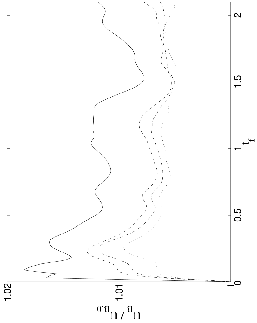
Figure 1: Time evolution of the total magnetic energy, $U_{B}$, normalized to the initial total magnetic energy $U_{\rm B,0}$, for models m3c1 ($\chi_{i0}=10^{-1}$, solid line), m3c2 ($\chi_{i0}=10^{-2}$, dash line), m3c3 ($\chi_{i0}=10^{-3}$, dot-dash line), and m3c4 ($\chi_{i0}=10^{-4}$, dotted line). The systems settle into approximate equilibrium states for $t\gtrsim t_{f}$.

The convergence study performed in this section deals solely with globally-integrated quantities, such as the total magnetic energy. Figure 1 shows the results of a study of $\chi_{i0}$-convergence, in which we carried out runs with $\chi_{i0}=10^{-1}$, 10^-2, 10^-3, and 10^-4 on a $256^{3}$ grid with ${\cal M}=3$. These four models show a similar evolution pattern, with an initial jump in the magnetic energy due to the initial perturbation followed by evolution to a quasi-equilibrium with a fluctuating magnetic energy. Fluctuations in the magnetic energy in AD turbulence have been observed in other simulations as well (e.g. Hawley & Stone, 1998). These fluctuations appear to be random, and they prevent us from carrying out a precise convergence study; in particular, we find that runs at different resolutions or with different values of $\chi_{i0}$ yield different time histories of the fluctuations.

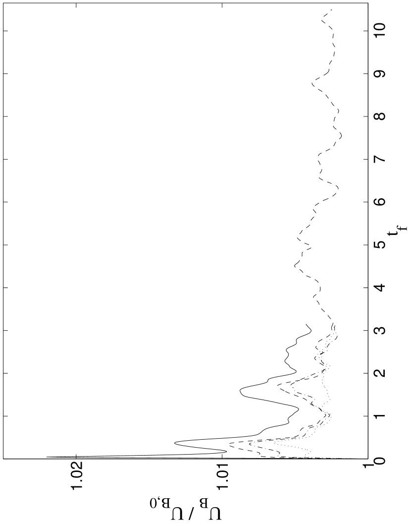
Figure 2: Time evolution of the total magnetic energy, $U_{B}$, for four 128³ turbulence models with the same initial conditions (models m3c1 to m3c4). One of the models (m3c2, with $\chi_{i0}=10^{-2}$) runs until $t>10t_{f}$. The system is approximately in equilibrium for $t\gtrsim t_{f}$, with random fluctuations.

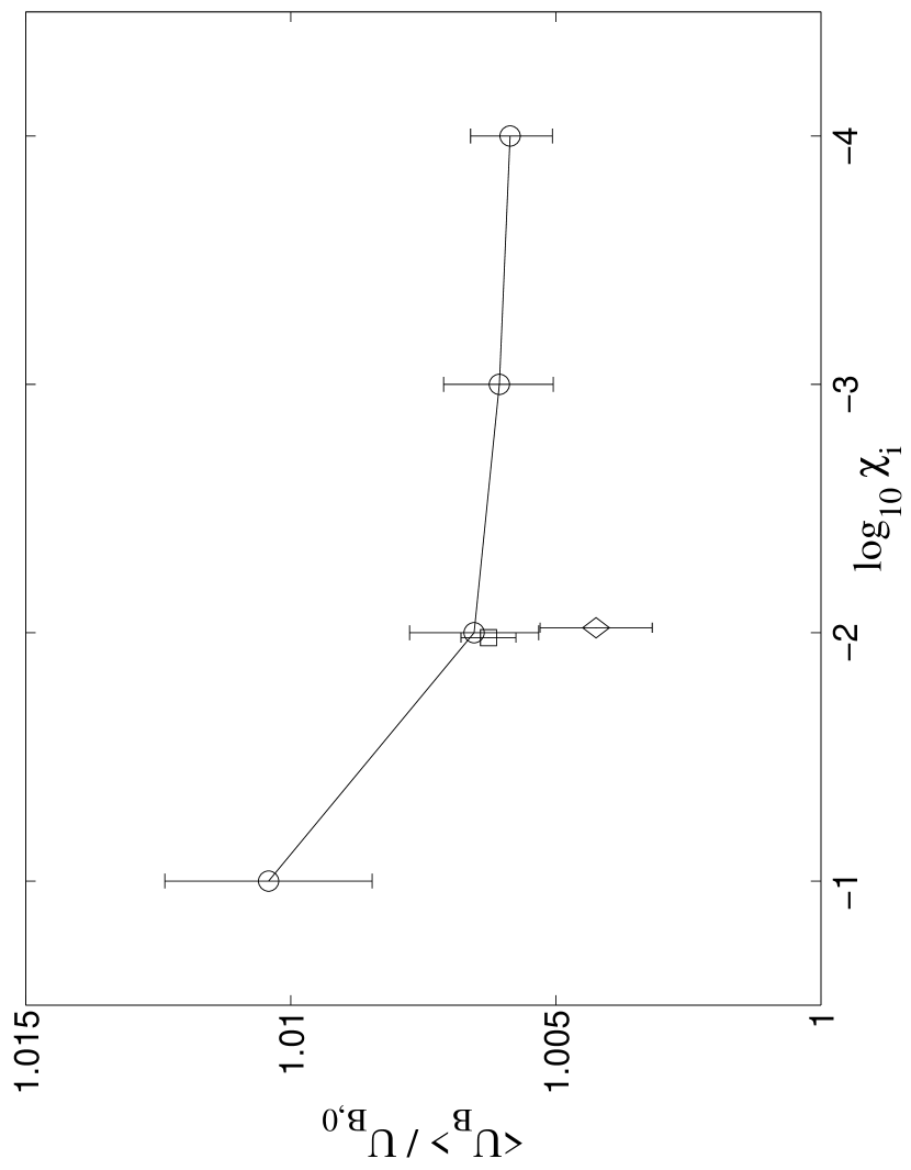
Figure 3: Convergence behavior of the time-averaged total magnetic energy, $\langle U_{B}\rangle$, for models m3c1 to m3c4 as a function of $\chi_{i0}$. The total magnetic energies (circles) are averaged after the first crossing time and the error bars show the standard errors of the means. The total magnetic energy is converged within the fluctuation limits for an ionization mass faction $\chi_{i0}\leq 10^{-2}$. The total magnetic energy of two models with the same initial conditions of the model m3c2 but with resolution of 128³ (diamond) and 512³ (square) are also plotted. The $\chi_{i0}$ of these two models are the same as m3c2 but changed here by a small amount in the plotting for the clarity of the overlapping error bars.

In order to address the issue of convergence in simulation time, we ran the model m3c2 on a $128^{3}$ grid for a simulation time $>10t_{f}$; such a long run is prohibitive using a $256^{3}$ grid. The flow time is defined as $t_{f}\equiv l_{0}/v_{\rm rms}$. The time history of the magnetic energy is shown in Figure 2. We see that the system is approximately in an equilibrium state after one flow time $t_{f}$, and that the fluctuations persist without a clear period. Since the time to reach an equilibrium state is about $t_{f}$, we continued the $\chi_{i0}$-convergence simulations for a time somewhat more than $2t_{f}$. The mean and standard deviation of the magnetic energy determined after the first crossing time are shown in Figure 3. We can see that the total magnetic energy converges quickly as $\chi_{i0}$ decreases. The variation of the mean magnetic energy among the models with $\chi_{i0}=10^{-2}$ to $10^{-4}$ is well within the amplitude of the fluctuations, but the error in the model with $\chi_{i0}=10^{-1}$ is larger than this. We conclude that the results are converged for $\chi_{i0}\lesssim 10^{-2}$. In Paper I we showed that the heavy-ion approximation is satisfied if the AD Reynolds number, $R_{\rm AD}$, is large compared to ${{\cal M}_{{\rm A}i}}^{2}$ (eq. 11). In a turbulent box simulation, it is not trivial to define ${{\cal M}_{{\rm A}i}}$ or $R_{\rm AD}$ because of the intermittency of turbulence. After driving the box for a period of time, the local ${{\cal M}_{{\rm A}i}}$ and $R_{\rm AD}$ have enormous variations—for example, in the Mach 10 model with $\chi_{i0}$ = $10^{-3}$, locally defined values of $R_{\rm AD}(\ell_{v_{i}})$ vary by a factor of 10¹⁴! Therefore, we compute the volume mean $\langle R_{\rm AD}\rangle_{V}$ for both ions and neutrals, using the length scale defined in equation (10), and list them in Table 1. The time at which these volume means are evaluated is also listed in the table. Values of $\langle R_{\rm AD}\rangle_{V}$ fluctuate, but vary by less than a factor of two for $t>t_{f}$ for both the Mach 3 and the Mach 10 models. From Table 1, we see that the requirement to achieve a converged solution is actually ${{\cal M}_{{\rm A}i}}^{2}/\langle R_{\rm AD}(\ell_{v_{i}})\rangle_{V}\lesssim 0.03$; this is well satisfied for $\chi_{i0}$ = 10^-2, which accounts for the accuracy of the models with $\chi_{i0}=10^{-2}$ in Figure 3. Note that the AD Reynolds number $R_{\rm AD}(\ell_{0})$ evaluated on the scale of the box is significantly larger than $\langle R_{\rm AD}(\ell_{v_{i}})\rangle_{V}$, so having ${{\cal M}_{{\rm A}i}}^{2}/R_{\rm AD}(\ell_{0})\ll 1$ (or even $\lesssim 0.03$) is not sufficient for the validity of the heavy ion approximation.

To determine the spatial resolution required for turbulent AD simulations, we ran models with 128³ and 512³ grid cells and with the same initial conditions as model m3c2. The total magnetic energies of these two models are plotted in Figure 3 alongside that of the 256³ model. The total magnetic energy, as well as other physical quantities, are converged at a resolution of 256³ using ZEUS-MPAD.

From these convergence studies, we conclude that we can use the heavy-ion approximation with $\chi_{i0}=10^{-2}$ to simulate systems with true values of $\chi_{i0}\lesssim 10^{-6}$. A spatial resolution of at least $256^{3}$ is needed. To obtain reliable statistical results, we suggest driving the system for more than 1 one flow time before measuring the physical quantities of the system.

5 Power Spectra

The recent work of Oishi & Mac Low (2006) on MHD turbulence simulations with AD compared the magnetic energy spectra with and without ambipolar diffusion and concluded that AD produces no dissipation range in the magnetic energy spectrum. In this section, we carry out a detailed investigation of velocity and magnetic field power spectra and show that AD does in fact have a small, but detectable, effect on the magnetic energy spectrum.

Generally, for an isotropic turbulent flow, the velocity power spectrum is computed using $P_{v}(k)=\Sigma\hat{u}_{i}(k)\hat{u}_{i}^{*}(k)$, where $\hat{u}_{i}(k)$ is the Fourier transform of the $i^{\rm th}$ component of velocity $u_{i}$(r) and the sum is over all three velocity components and all wave numbers ${\bf k}$ in the 3D shell $k\leq|{\bf k}|<k+dk$. The inertial range of the power spectrum is expected to be a power law $P(k)\sim k^{-n}$. For Kolmogorov (Kolmogorov, 1941) and Burgers (Burgers, 1974) power spectra, $n=5/3$ and 2, respectively. Because of the relatively strong magnetic field for $\beta$ = 0.1, especially in our low Mach number models, highly anisotropic distributions are expected. It is therefore necessary to compute both $P_{v}(k_{r})$ and $P_{v}(k_{z})$, the Fourier component power spectra perpendicular and parallel to the mean magnetic field, respectively, where $k_{r}=\sqrt{k_{x}^{2}+k_{y}^{2}}$. For example, $P_{v}(k_{r})=\Sigma\hat{u}_{i}(k_{r})\hat{u}_{i}^{*}(k_{r})$ where the sum is over all three velocity components and all wave numbers ${\bf k}_{r}$ in the 2D shell $k_{r}\leq|{\bf k}_{r}|<k_{r}+dk_{r}$ on the $x-y$ plane and over all planes along the cylinder with axis $z$. The magnetic field power spectrum is calculated in the same manner.

Theoretical work on incompressible ideal MHD turbulence in a strong magnetic field (e.g. Goldreich & Sridhar, 1995, 1997; Maron & Goldreich, 2001) concludes that $P_{v}(k_{\perp})\sim k_{\perp}^{-5/3}$, where $k_{\perp}$ is perpendicular to the local magnetic field; this has the same exponent as the Kolmogorov spectrum. We express this in terms of the exponent in the power spectrum as $n_{vi}(k_{\perp})\simeq 5/3$, where we have included the subscript “$i$” to indicate that this applies to the ions. However, numerical simulations (Maron & Goldreich, 2001; Müller et al., 2003; Boldyrev, 2005; Beresnyak & Lazarian, 2006) give a flatter spectrum that appears consistent with the Iroshnikov-Kraichnan spectrum, $n_{vi}(k_{\perp})=3/2$ (Iroshnikov, 1963; Kraichnan, 1965). It is computationally much easier to calculate $P_{v}(k_{r})$ than $P_{v}(k_{\perp})$, and fortunately the two are in close agreement because $k_{r}\approx k_{\perp}[1+O(\theta^{2})]$. On the other hand, $P_{v}(k_{\parallel})$ is not similar to $P_{v}(k_{z})$ because $k_{z}\approx\theta k_{\perp}$, where $\theta$ is the angle between the local magnetic field and the $z$-direction (Maron & Goldreich, 2001), so we shall not discuss $P_{v}(k_{z})$. Since the $k_{z}$ spectra are often not very meaningful, we also calculate the power spectra in terms of the total wavenumber, $P(k)$. These spectra are also of interest because observers do not have information on the true direction of the magnetic field. Any measurements of turbulent flows inside MCs will be restricted to the line of sight, which can be treated as a random direction from the true magnetic field direction. We have demonstrated this by computing the power spectra $P_{v}(k_{60})$ and $P_{B}(k_{60})$ at 60$\arcdeg$ from the $z$-axis (the median value of the angle relative to the field) for the ideal MHD model m3i, and we find that they agree with the combined power spectra $P_{v}(k)$ and $P_{B}(k)$ to within the uncertainties.

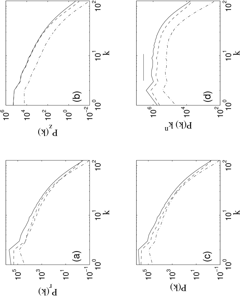
Figure 4: (a) Velocity power spectra of the neutrals ($n_{vn,r}$, solid line) and ions ($n_{vi,r}$, dashed line) and the magnetic field power spectrum ($n_{B,r}$, dot-dash line), all perpendicular to the global magnetic field for model m3c2. (b) Same as (a) but the components are parallel to the global magnetic field. The ions and neutrals have very similar spectra parallel to the global magnetic field direction since only weak fields are induced in the perpendicular direction. (c) The combined 3D velocity power spectra of neutrals ($n_{vn}$, solid line) and ions ($n_{vi}$, dashed line), and the power spectrum of the magnetic field ($n_{B}$, dot-dash line). (d) The compensated 3D velocity power spectra of neutrals (solid line) and ions (dashed line), and the compensated magnetic field power spectrum (dot-dash line). The power law indexes used for the compensation are listed in Table 2.

In Figure 4, we present the time-averaged power spectra of the ion velocity and magnetic field for model m3c2 in the time interval $\sim(1-3)t_{f}$. Because of the limited resolution (256³), we do not expect the inertial range to extend much beyond $k$ = 10, which corresponds to $k_{\rm phys}\Delta x\simeq 0.25$. Since the driving occurs between $k$ = 1 and 2, we have chosen to infer the power-law index by a least-squares fitting of the power spectrum from $k$ = 3 to 10. The uncertainty in the index is given by the standard error of the mean, which we calculate as the standard deviation evaluated for a total 14 data sets between $1-3t_{f}$ divided by the square root of the number of independent samples of the index, which we estimate as 3. In order to determine how long it takes for the turbulence system to become uncorrelated, we continued models m3i and m3c2 to a time somewhat greater than 5$t_{f}$. By studying the density correlation between data sets at different times, we found that they become essentially uncorrelated in a time slightly less than $t_{f}$. We therefore take the number of independent samples to be the largest integer in $t_{\rm run}/t_{f}$. For data sets dumped out between $1-3t_{f}$, we shall have 3 independent samples. The range of wavenumbers used to determine the power-law index of the power spectrum is very narrow, so we carried out a high-resolution run with a resolution of $512^{3}$ (labeled m3c2h) and found that the power-law indexes agreed with those from the $256^{3}$ simulation within the errors. We conclude that, although the results for the $256^{3}$ runs may not represent accurately the values for the physical case in which the inertial range extends over many decades. these results can be used to study the dependence of the indexes on the underlying physical parameters.

No time evolution of the power-law indexes is apparent for $t>t_{f}$: the time-averaged power indexes between $t_{f}$ and $2t_{f}$ agree with those between $2t_{f}$ and $3t_{f}$ within the uncertainties. Figure 4a shows the power spectra, $P_{v,r}(k)$ and $P_{B,r}(k)$, of the of the velocity, $v_{r}$, and magnetic field, $B_{r}$, perpendicular to the global magnetic field. Both ion and neutral velocity spectra are shown. The close agreement between $P_{vi,r}(k)$ and $P_{B,r}(k)$ is consistent with equipartition between the ion kinetic and magnetic energy perpendicular to the mean field (Zweibel & McKee, 1995; but see §7 below). Figure 4b shows the power spectra of the velocity and magnetic field parallel to the global magnetic field, $P_{v,z}(k)$ and $P_{B,z}(k)$. The power spectra for neutral and ion velocities parallel to the global field are about the same because the weakness of the magnetic forces in this direction implies that the ions and neutrals are well coupled. Figure 4c shows the combined power spectra $P(k)$ for the neutral and ion velocities and for the magnetic field. The power-law indexes resulting from a least-squares fit to these spectra are listed in Table 2 and are used to produce the compensated versions of these spectra in Figure 4d.

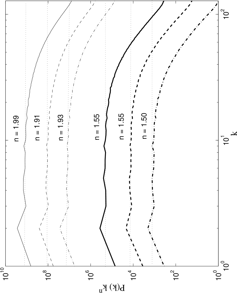
Figure 5: The compensated power spectra of models m3c1 ($\chi_{i0}=10^{-1}$, solid line), m3c2 ($\chi_{i0}=10^{-2}$, dashed line), and m3c3 ($\chi_{i0}=10^{-3}$, dot-dash line). The spectra are compensated by the power law indexes of the inertial range fitted between $k=3-10$. The thin lines are neutral velocity spectra and the thick lines are the magnetic field power spectra. The spectra are shifted up and down for side-by-side comparison. As shown in the figure and listed in Table 2, the power law indexes are not sensitive to the choice of ionization mass fraction $\chi_{i0}$, even for $\chi_{i0}$ as large as 0.1.

First, we look at the $\chi_{i0}$-convergence of the power spectra, using the heavy-ion approximation. As shown in Table 2, the power-law indexes of the four models m3c1 to m3c4, which have $\chi_{i0}=10^{-1}-10^{-4}$, are similar within the uncertainties. Figure 5 shows this result graphically. Interestingly, the correct value of the power-law index can be obtained with $\chi_{i0}=0.1$ even though we found in §4 that convergence in magnetic field energy required $\chi_{i0}\lesssim 0.01$. This lack of sensitivity to the value of $\chi_{i0}$ could be because the relatively low resolution of the simulations and the intrinsic fluctuations discussed above lead to significant uncertainties in determining the power-law indexes.

Next, we investigate whether driving the neutrals alone would alter the power spectrum of the ion (model m3c2a). In this case, the motion of the ions is mainly due to the drag force exerted by the neutrals. The spectral indexes are basically the same as in model m3c2, in which both the ions and the neutrals are driven (see Table 2). We conclude that our results are insensitive to whether the driving applies to both the neutrals and ions or to the neutrals alone.

How do the spectral indexes depend on the AD Reynolds number? Oishi & Mac Low (2006) addressed this question by comparing a run with $R_{\rm AD}(\ell_{0}/4)=1$ to an ideal MHD run, both at Mach 10. From visual inspection of their results, they did not find any significant difference in the magnetic power spectra [$n_{B}(k)$—see their figure 3]. By contrast, when they compared a simulation with ohmic dissipation to an ideal MHD simulation, they found a large difference in the power spectra. We performed three Mach 10 simulations with AD (models m10c1 to m10c3) using the same initial conditions as in Oishi & Mac Low (2006) and a Mach 10 ideal MHD model m10i for comparison. The ionization mass fraction, $\chi_{i}$, in model m10c1 is 0.1, which is the same as in the AD model of Oishi & Mac Low (2006). Unfortunately, due to the low densities created in highly supersonic turbulence, it is computationally too expensive to continue the Mach 10 models much beyond $t=t_{f}$. Therefore, we obtained only one snapshot of the turbulence for each case of the Mach 10 turbulence with AD, which is insufficient to determine the uncertainty in the indexes.

We then carried out a quantitative comparison between the AD models and an ideal model at Mach 3. The magnetic spectral index for Model m3i, an ideal MHD model with the same initial condition as the AD model m3c2, is $n_{B}(k)=1.25\pm$0.09, which is clearly flatter than the value 1.55$\pm$0.12 for the AD model. We confirmed this result by comparing a high-resolution ideal MHD model (m3ih at 512³ resolution) with the high-resolution AD model m3c2h. However, the effect due to AD is much smaller than that of ohmic diffusion as reported in Oishi & Mac Low (2006).

More generally, as shown in Table 3, the spectral indexes change systematically with the AD Reynolds number. All the indexes listed undergo a statistically significant increase in going from the ideal MHD case to the strongest AD case [$R_{\rm AD}(\ell_{0})=0.12$]. The indexes for the neutral velocity increase down to the lowest value of $R_{\rm AD}$, becoming slightly greater than 2; presumably they level off at yet lower values of $R_{\rm AD}$, since they approach Burgers value of 2 in the hydrodynamic limit (Padoan et al., 2007). The index for the $z$-component of the ion velocity [$n_{vi,z}(k)$] is locked to that of the neutral velocity since the ions and neutrals are well-coupled parallel to the field. With the exception of $n_{vi,z}$, all the ion and magnetic field indexes approach constant values at low $R_{\rm AD}$, although the value of $R_{\rm AD}$ at which they level off varies. At the lowest value of $R_{\rm AD}$, the index for the magnetic field has the Iroshnikov-Kraichnan value, $n_{B}(k)=1.50\pm 0.10$, as expected for strong-field (i.e., low-${{\cal M}_{\rm A}}$) turbulence (Maron & Goldreich, 2001; Müller et al., 2003; Boldyrev, 2005; Beresnyak & Lazarian, 2006). However, the effect of the neutrals on the ions is still apparent in this strong AD case, since the ion velocity indexes differ significantly from the ideal MHD values. This is to be expected, since in the ideal MHD simulation, the power spectrum in the ion fluctuations at small scales is due entirely to a cascade from larger scales, whereas in the AD simulations the ions are driven at all scales by interactions with the dominant neutrals. Therefore, for $R_{\rm AD}(\ell_{0})\lesssim 1$, the power spectra of the neutral velocities and of at least the $z$-component of the ion velocity is close to a Burgers spectrum, and the power spectrum of the magnetic field is close to the Iroshnikov-Kraichnan spectrum.

Passot et al. (1988) pointed out that the observed linewidth-size scaling, $\sigma_{v}\propto\ell^{1/2}$ (e.g. Solomon et al., 1987), is what would be predicted for Burgers turbulence. Padoan et al. (2000) explained this as the result of ideal MHD turbulence in a weakly magnetized, supersonic (and hence super-Alfv$\acute{\rm e}$nic) medium. Our results show that the Burgers spectrum can be obtained even in sub-Alfv$\acute{\rm e}$nic turbulence if the AD effect is strong. However, it must be borne in mind that our results apply to the inertial range in $256^{3}$ simulations, and as discussed above they differ by an unknown amount from the physical case with a far larger inertial range. Furthermore, the run with the lowest AD Reynolds number, $R_{\rm AD}({\ell_{vi}})=0.015$, has a value of ${{\cal M}_{{\rm A}i}}^{2}/R_{\rm AD}({\ell_{vi}})$ comparable to that for the $\chi_{i0}=0.1$ runs, which are known to be not fully converged; hence, we cannot be sure that this run is fully converged either. The trends should be reliable, however.

6 Probability Density Function

The probability density function (PDF) for the density of supersonic, isothermal turbulence is log-normal (V$\acute{\rm a}$zquez-Semadeni, 1994). That is, the volume-weighted or mass-weighted probability that the density has a given value is

$$f_{V,\,M}\propto\exp[-(x\pm\mu_{x})^{2}/2\sigma_{x}^{2}],$$ (13)

where $x\equiv\ln(\rho/\bar{\rho})$, $\mu_{x}=\sigma_{x}^{2}/2$, and the plus and minus signs refer to the volume-weighted and mass-weighed probabilities, respectively (e.g., McKee & Ostriker, 2007). Hence, the standard deviation of the distribution, $\sigma_{x}$, is related to the means by

$${\langle x\rangle}_{M}=-{\langle x\rangle}_{V}=\frac{1}{2}\sigma_{x}^{2}.$$ (14)

Table 4 gives the values for these quantities and for the median of $-x$ (labeled $-\tilde{x}$) for a range of values of $R_{\rm AD}(\ell_{0})$, extending from ideal MHD [$R_{\rm AD}(\ell_{0})\rightarrow\infty$] to almost decoupled [$R_{\rm AD}(\ell_{0})=0.12$]. All these quantities should be equal for a log-normal PDF, and indeed they agree to within the uncertainties, demonstrating that the log-normal behavior of the PDF is preserved in the case of ambipolar diffusion. (Note that the equality of the median and the mean confirms only that the PDF is symmetric, not that it is a log-normal.)

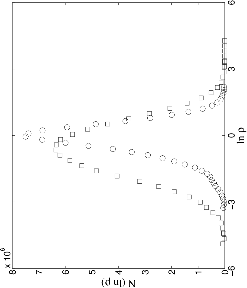
Figure 6: Density PDF of ideal MHD model m3i (circles) and model m3c2 (squares). The density PDF of model m3c2 shows significantly larger dispersion than the ideal MHD model because of the effects of ambipolar diffusion. The dispersion and mean of the PDFs are listed in Table 4.

Table 4 shows, and Figure 6 confirms, that the width of the density PDF increases as AD becomes more important, although our results do not show a monotonic behavior. This increase is plausible due to the decreasing ability of the magnetic field to cushion the shocks as $R_{\rm AD}(\ell_{0})$ decreases. For very small $R_{\rm AD}(\ell_{0})$, we expect the dispersion to approach the hydrodynamic value,

$$\sigma_{x}^{2}={\rm ln}(1+\frac{1}{4}{\cal M}^{2})$$ (15)

(Padoan & Nordlund, 2002). This corresponds to $\sigma_{x}^{2}/2=0.59$ for ${\cal M}=3$, which is consistent with our run at the lowest value of $R_{\rm AD}(\ell_{0})$. For the ideal MHD case, Padoan et al. (2007) find a similar relation with the sonic Mach number replaced by the Alfv$\acute{\rm e}$n Mach number. Ostriker et al. (2001) do not find such a relation for this case, nor do we. It must be borne in mind that the simulations of Ostriker et al. (2001) had a range of values of $\beta$, and that our simulations all have $\beta=0.1$, which is substantially smaller than the value in the super-Alfv$\acute{\rm e}$nic simulations of Padoan et al. (2007); in addition, our resolution is substantially less.

7 Scaling with $R_{\rm AD}$

As we have seen in §5 and §6, the statistical properties of the turbulent box vary as the AD Reynolds number of the system, $R_{\rm AD}(\ell_{0})$, changes from the ideal MHD case to the strong AD cases. Here we shall examine several other properties as functions of $R_{\rm AD}(\ell_{0})$.

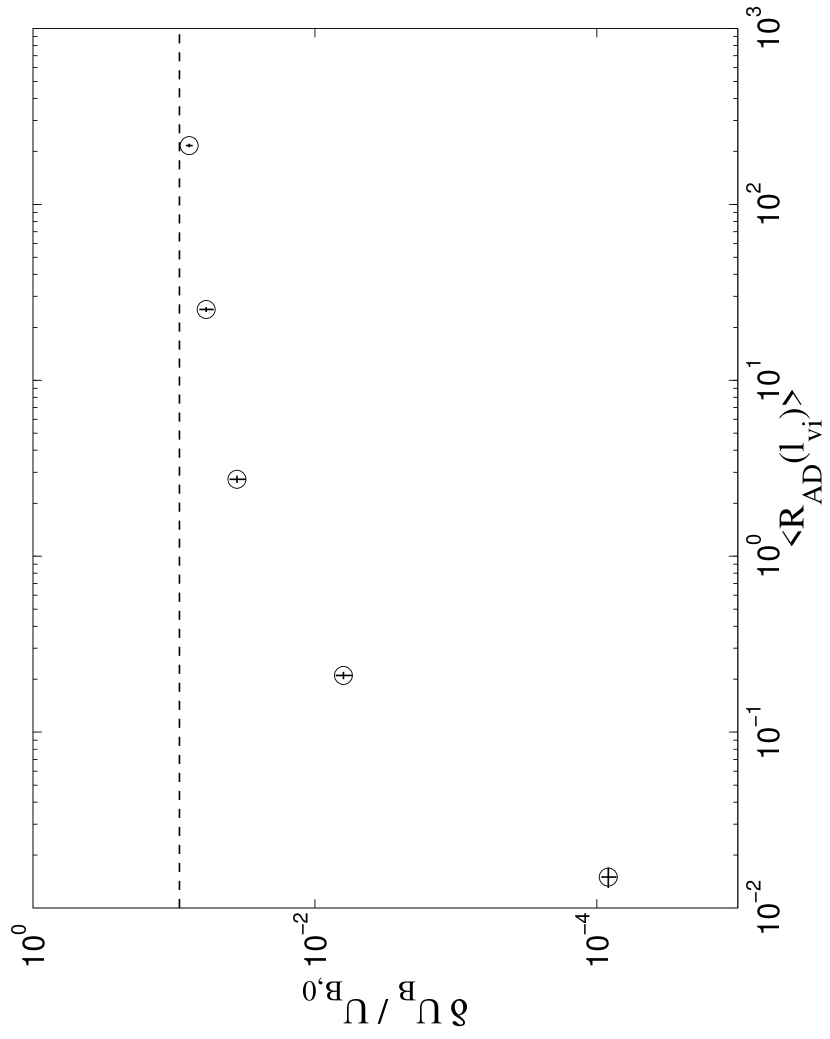
Figure 7: Time-averaged change in the normalized total magnetic energy, $\delta U_{B}/U_{B0}$ for five models m3c2r-1 to m3c2r3 as a function of $R_{\rm AD}(\ell_{v_{i}})$. Uncertainties are shown as error bars. The dashed line is $\delta U_{B}/U_{B0}$ for the ideal MHD model m3i. With increasing $R_{\rm AD}$, $\delta U_{B}/U_{B0}$ approaches the ideal MHD model value.

In the convergence study in §4, we used the total magnetic energy of the system to gauge the convergence in terms of spatial resolution and of ionization mass fraction, $\chi_{i0}$. Using the initial magnetic energy of the system as a reference, we can see how the fluctuating magnetic energy of the system, $\delta U_{B}=U_{B}-U_{B_{0}}$, changes as a function of $R_{\rm AD}$. Figure 7 shows that when $R_{\rm AD}$ is small, $\delta U_{B}$ is also small; indeed, when $R_{\rm AD}$ approaches zero, that is when the ion fluid is totally decoupled from the neutral fluid, $\delta U_{B}$ should approach the value appropriate for the driven ions (recall that we drive both ions and neutrals). Were we to drive only the neutrals, $\delta U_{B}$ would approach zero as $R_{\rm AD}\rightarrow 0$.

On the other hand, when $R_{\rm AD}$ increases, $\delta U_{B}$ increases to the value appropriate for an ideal MHD system. Since MHD waves have equipartition between the kinetic energy normal to the field, $(1/2)\rho v_{\perp}^{2}$, and the perturbed magnetic energy, $\delta U_{B}$, we expect $\delta U_{B}/U_{B0}=(2/3){{\cal M}_{\rm A}}^{2}$, under the assumption that the velocities are isotropic. Indeed, in their low-$\beta$ runs, Stone et al. (1998) found $\delta U_{B}/U_{B0}\simeq 0.6{{\cal M}_{\rm A}}^{2}$, consistent with this expectation. For our models, ${{\cal M}_{\rm A}}^{2}=\beta{\cal M}^{2}/2=9/20$, so the theoretical expectation is $\delta U_{B}/U_{B0}=0.3$. We find a significantly smaller value, however, $\delta U_{B}/U_{B0}\simeq 0.1$. We attribute this to our boundary conditions: it is possible to have significant kinetic energy that does not perturb the field, in the form of eddies rotating around the field lines or flows along field lines. This effect was much smaller for Stone et al. (1998) since they had a much smaller driving scale, peaked at $k=8$. To see whether this effect could be significant in our models, we evaluated ${\langle{\bf v}\rangle}^{2}$, where the average is over time and the results are summed over all cells in the box. One would expect this to be close to zero, whereas we found it to be a significant fraction of ${\langle v^{2}\rangle}$. Since these motions are at $k\sim 1$, however, they do not affect the power spectra.

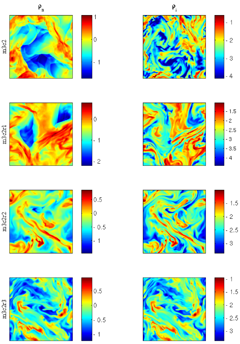
Figure 8: Logarithmic density (log$\rho$) slices of models m3c2 (1st row), m3c2r1 (2nd row), m3c2r2 (3rd row), and m3c2r3 (4th row) at the middle of the turbulent box normal to the $z$-direction at time $t=3t_{f}$. The left column shows the neutral density and the right column shows the ion density. When $\langle R_{\rm AD}\rangle_{V}$ is large, the ions and neutrals are sufficiently strongly coupled that they evolve like a single fluid.

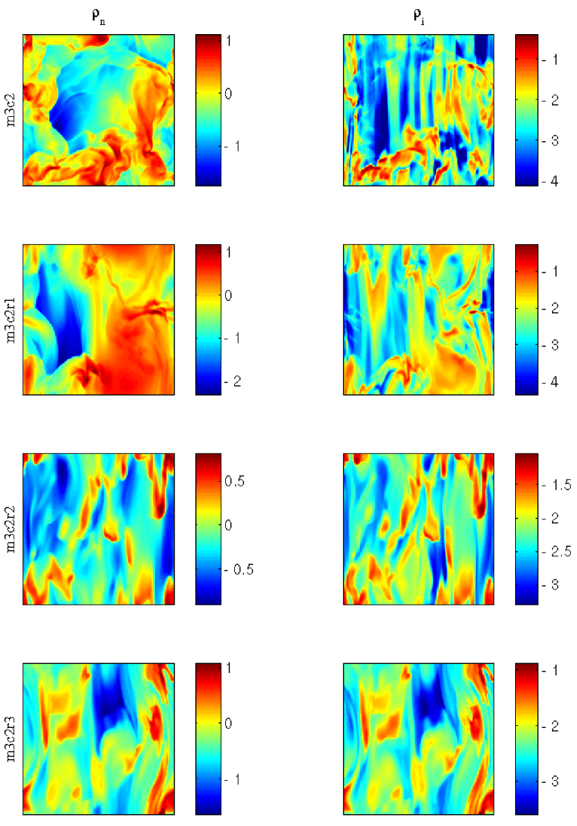
Figure 9: Same as Figure 8 but the slices are at the middle of the turbulent box normal to the $y$-direction. The ion density is highly anisotropic due to the strong magnetic field and relatively weak turbulence (${{\cal M}_{\rm A}}<1$).

Figures 8 and 9 show density slices for the ions and neutrals normal to the $z$ and $y$ axes, respectively, for models m3c2, m3c2r1, m3c2r2, and m3cr3 at $t=3t_{f}$. We see that the coupling between ions and neutrals gets stronger with larger $R_{\rm AD}$. In Model m3c2r3, which has $R_{\rm AD}(\ell_{0})=1200$ and is very close to ideal MHD, the coupling between the ions and neutrals is so strong that there is hardly any difference between the spatial distributions of their densities.

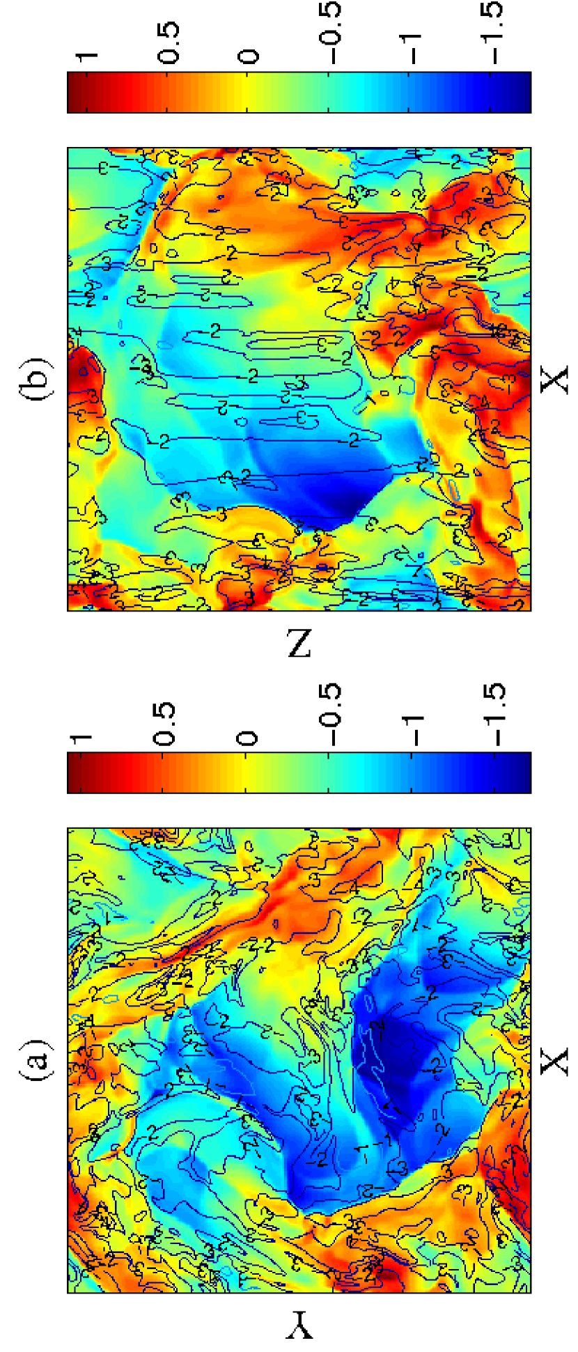
Figure 10: Spatial distribution of ionization mass fraction $\chi_{i}$. (a) The $\chi_{i}$ of a slice at the middle of the turbulence box normal to the z-direction (B-field direction). The contours are log $\chi_{i}$ and the grey scale (color scale in online version) map is log $\rho_{n}$. Small $\chi_{i}$ regions usally associate with high density regions. (b) Same as (a) but the slice is normal to the y-direction. The contours are highly anisotropic because of the restraint of ions due to strong magnetic field.

As mentioned above, supersonic turbulence quickly creates large density contrasts in the system. In the presence of AD, it also creates large ionization contrasts, as can be inferred from Figures 8 and 9. Figures 10a and 10b show the ionization mass fraction $\chi_{i}$ of a slice at the middle of the turbulence box normal to the $z$ and $y$ axes, respectively, from the model m3c2 at time $t=3t_{f}$. Regions of low ionization are found to occur in regions of high density: Ambipolar diffusion allows shocks to compress the neutrals much more than the ions. Because we have assumed overall ion conservation, the mass of ions on a given flux tube is constant in the absence of numerical diffusion. Therefore, the change in $\chi_{i}$ is purely a dynamical result. Furthermore, the contours of $\log\rho_{i}$ are highly anisotropic and are aligned with the $z$-axis, as shown in Figure 10b.

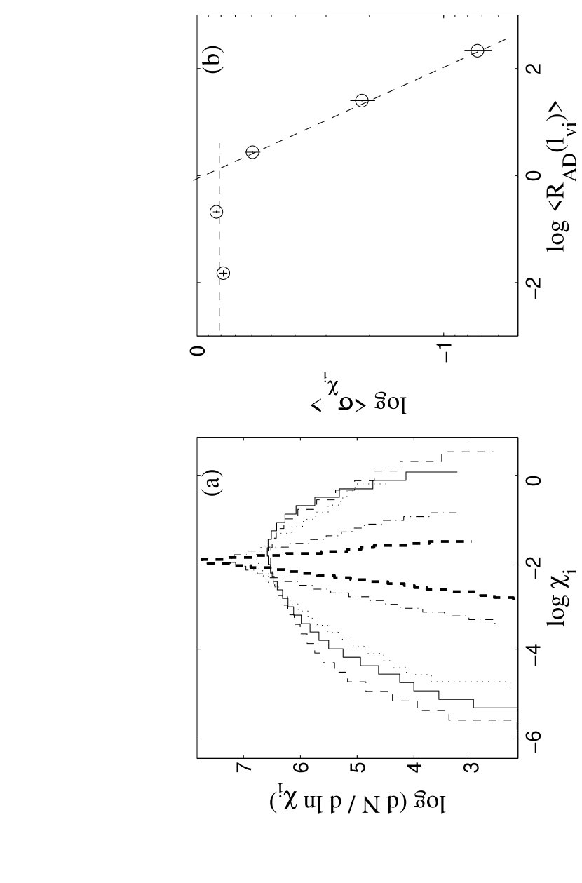
Figure 11: $R_{\rm AD}$ effects: (a) The PDFs of $\chi_{i}$ for models m3c2r-1 (solid), m3c2 (dash), m3c2r1 (dotted), m3c2r2 (dot-dash), and m3c2r3 (thick dash) at t = 3$t_{f}$ as a function of $\langle R_{\rm AD}(\ell_{v_{i}})\rangle_{V}$. (b) The time-averaged dispersions of the $\chi_{i}$ distributions for the five models versus $\langle R_{\rm AD}(\ell_{v_{i}})\rangle_{V}$ over 2 $t_{f}$. The $\chi_{i}$ and $\langle R_{\rm AD}(\ell_{v_{i}})\rangle_{V}$ show a power law relation when the $\langle R_{\rm AD}(\ell_{v_{i}})\rangle_{V}>$ 1. When $\langle R_{\rm AD}(\ell_{v_{i}})\rangle_{V}<$ 1, the dispersion of $\chi_{i}$ approaches a constant.

The dispersion in the ionization changes systematically with $R_{\rm AD}$. Figure 11a shows the distribution of $\chi_{i}$ for five models, from m3cr-1 to m3c2r3, at $t=3t_{f}$. We can see that$\chi_{i}$ has a larger dispersion for smaller values of $R_{\rm AD}$. This is to be expected, because in the ideal MHD case ($R_{\rm AD}=\infty$), $\chi_{i}$ will maintain a single value for the whole turbulent box, since the ions and neutrals are perfectly coupled. With smaller values of $R_{\rm AD}$, the ions start to decouple from the neutrals and the dispersion in $\chi_{i}$ increases. We plot the dispersion of $\chi_{i}$ in Figure 11b. The dispersion decreases as a power of $R_{\rm AD}$ for models m3c2r1, m3c2r2, and m3cr3, which have $\langle R_{\rm AD}(\ell_{v_{i}})\rangle_{V}>1$, and then becomes approximately constant for the two models with $\langle R_{\rm AD}(\ell_{v_{i}})\rangle_{V}<1$. The turning point is roughly located at $\langle R_{\rm AD}(\ell_{v_{i}})\rangle_{V}\sim 1$. The dispersion in the ionization is somewhat larger than the dispersion in the neutral density, even at the smallest values of $R_{\rm AD}$ we have simulated, since it includes the dispersion in both the neutral density and the ion density.

8 Discussion and Conclusions

Magnetic fields are an important ingredient in the interstellar medium and are believed to play an important role in star formation. On large scales, the magnetic field is frozen to the gas, and ideal MHD is appropriate. Indeed, to date almost all 3D simulations of MHD turbulence are based on the assumption of ideal MHD. On smaller scales, ambipolar diffusion (AD) becomes significant, and in a turbulent medium, the AD lengthscale ${\ell_{\rm AD}}$ varies substantially due to high contrasts in density, velocity, and magnetic fields. When the average value of ${\ell_{\rm AD}}$ is comparable to or larger than the size of the turbulent box—i.e., when the AD Reynolds number of the box $R_{\rm AD}(\ell_{0})\lesssim 1$—AD can significantly alter the properties of the turbulence. Simulating this effect is computationally challenging, however, since the timestep required in explicit codes is proportional to both the square of the gridsize, $\Delta x^{2}$, and to the square root of the ionization mass fraction, $\chi_{i0}$, both of which are exceedingly small for accurate modeling of MCs. Semi-implicit treatments can avoid the problem with $\Delta x^{2}$ but not the one with the small ionization mass fraction. To overcome the latter problem, Oishi & Mac Low (2006) adopted an artificially high value for the ionization mass fraction, $\chi_{i0}=0.1$, and a correspondingly low value for the ion-neutral coupling coefficient, ${\gamma_{\rm AD}}$, in carrying out the 3D simulation for a turbulent medium with ambipolar diffusion. Li et al. (2006) independently developed this approximation, which they termed the heavy-ion approximation, and determined the condition for its validity by testing it on several classical MHD problems involving AD.

In this paper, we report the results of our simulations of sub-Alfv$\acute{\rm e}$nic turbulence with AD using the heavy-ion approximation. We assume that the ions are conserved, but in the Appendix we show that our results also apply approximately to the case of time-dependent ionization for realistic molecular densities. Our models focus on the case of a thermal Mach number of 3 and a plasma $\beta$ of 0.1, corresponding to an Alfv$\acute{\rm e}$n Mach number ${\cal M}_{A}=0.67$. By using this relatively low value of the Mach number, we are able to perform a number of $256^{3}$ simulations with a duration of $3-5t_{f}$, where $t_{f}=\ell_{0}/v_{\rm rms}$ is the flow time across the box. We find, in agreement with previous workers (e.g. Hawley & Stone, 1998), that simulations of turbulence with AD have significant fluctuations in most physical quantities, which makes it difficult to accurately determine the statistical properties of the system. We carried out several convergence studies to determine the validity of our simulations: First, we showed that independent samples of the turbulence can be obtained at time intervals $\simeq t_{f}$ beginning at $t=t_{f}$, and that a total running time of $\sim 3t_{f}$ is sufficient. Second, we showed that the results are converged to within the uncertainties for a spatial resolution of $256^{3}$. Finally, we showed that the heavy-ion approximation with $\chi_{i0}=10^{-2}$ can represent a $\chi_{i0}=10^{-6}$ system as observed in MCs with sufficient accuracy. This speeds up the calculation by a factor of about 100, but it is nonetheless a factor 10 slower than an ideal MHD simulation.

High-resolution ideal MHD turbulence simulations show that the velocity power spectrum for super-Alfv$\acute{\rm e}$nic turbulence will be close to a Burgers spectrum with a power index $n_{v}(k)\simeq 2$ (Padoan et al. 2007). If the turbulence is sub-Alfv$\acute{\rm e}$nic, the power spectrum will be highly anisotropic with respect to the direction of the magnetic field. Theoretical studies on incompressible turbulence suggest the velocity power spectrum normal to the magnetic field will be a Kolmogorov-like spectrum, with power index of 5/3 (e.g. Goldreich & Sridhar, 1995). Numerical simulations indicate that in strong fields the power index is close to 1.5 (i.e., at low values of ${{\cal M}_{\rm A}}$) (Maron & Goldreich, 2001; Müller et al., 2003), and that the 5/3 index is realized only for relatively weak mean fields (Boldyrev, 2005).

We have studied how the power spectra change as a function of the importance of ambipolar diffusion, which is measured by the AD Reynolds number $R_{\rm AD}$. We use two different values of the AD Reynolds number: $R_{\rm AD}(\ell_{0})$ is defined in terms of the box size and the rms velocity in the box, whereas $\langle R_{\rm AD}(\ell_{v_{i}})\rangle_{V}$ is the volume average of the AD Reynolds number defined in terms of local parameters, with a length equal to the scale over which the ion velocity varies. $\langle R_{\rm AD}(\ell_{v_{i}})\rangle_{V}$ is the quantity that enters the criterion to ensure the validity of the heavy-ion approximation (eq. 11). It varies with time during a simulation, but is constant to within a factor of 2 in the simulations reported here; once the system reaches equilibrium at $t\simeq t_{f}$, the change in $\langle R_{\rm AD}\rangle_{V}$ is $\lesssim 10\%$. For the five models with $\langle R_{\rm AD}(\ell_{v_{i}})\rangle_{V}$ from 0.015 to 215.83 [initial $R_{\rm AD}(\ell_{0})$ from 0.12 to 1200] that we have computed, we see a progressive transition of system properties from a model with a strong AD effect to a near ideal MHD model; we also computed ideal MHD models for comparison. All the power law indexes we computed increase in going from the ideal MHD case to the case of strongest AD, and most of them appear to approach a constant at small $R_{\rm AD}$.

For the ideal MHD case, we confirm that the power spectrum of the ion velocity normal to the field is consistent with the Iroshnikov-Kraichnan spectrum ($n_{vi,r}=1.5$), as found in previous studies of turbulence in strong fields. This index increases with the importance of AD; it is consistent with the Kolmogorov value in four of our AD models, but is larger for the case in which the AD is strongest. The perpendicular magnetic field power is usually larger than that of the parallel magnetic field power, and as a result the power-law index for the total field, $n_{B}(k)$, is about the same as that for the perpendicular components of the field, $n_{B,r}(k)$. We find that these power-law indexes are about 1.2 in the case of ideal MHD and rise to about 1.5 for the case in which AD is strongest. This does not agree with the conclusion of Oishi & Mac Low (2006), who found no difference in the magnetic power spectra of an ideal MHD model and models with strong AD. We note that the change in the index of the power spectra we find between ideal and AD-dominated MHD is small compared to the difference they reported between ideal MHD and MHD dominated by ohmic diffusion.

By comparing the volume-averaged value of $\ln\rho$, the mass-averaged value, the dispersion in values, and the median, all of which have equal magnitude for a log-normal PDF, we concluded that the density PDF is indeed log-normal for all the cases we considered. The dispersion increases systematically as AD increases in importance, and is consistent with the Padoan & Nordlund (2002) result for the strong AD cases.

An important result from our sub-Alfv$\acute{\rm e}$nic turbulence simulations with AD is that the neutral gas in systems with small $\beta$ (strong magnetic field) and strong AD (small $R_{\rm AD}$) behaves like that in systems with large $\beta$ (weak magnetic field) and no AD. In particular, the neutral-velocity power spectrum in a strongly magnetized medium with strong AD is approximately consistent with a Burgers spectrum [$n_{v}(k)\simeq 2$]. It is thus not possible to infer the strength of the magnetic field from observations of the power spectrum unless it is known that the observations are on a sufficiently large scale that AD is not important.

Appendix A ION CONSERVATION VERSUS TIME-DEPENDENT IONIZATION

The calculations we have discussed in this paper are based on the assumption that the number of ions is conserved. In fact, as the density changes, ionization and recombination will change the number of ions. The ionization timescale is

$$t_{\rm ion}=\frac{x_{e}}{\zeta_{\rm CR}}\simeq 100\left(\frac{x_{e}}{10^{-7}}\right)\left(\frac{3\times 10^{-17}}{\zeta_{\rm CR}}\right)~{}~{}~{}{\rm yr},$$ (A1)

where $x_{e}\equiv n_{e}/n_{\rm H}$ is the ionization number fraction and $\zeta_{\rm CR}$ is the ionization rate per H atom, which is inferred to be about $(2.5-5)\times 10^{-17}$ s^-1 in dense clouds (Dalgarno, 2006). The recombination time scale is $t_{\rm rec}=1/\alpha n_{e}$, where $\alpha$ is the relevant recombination coefficient. In equilibrium these two time scales are equal, which implies that the equilibrium ionization is

$$x_{e,\,\rm eq}=\left(\frac{\zeta_{\rm CR}}{\alpha n_{\rm H}}\right)^{1/2}\simeq 10^{-7}n_{\rm H,\,3}^{-1/2},$$ (A2)

where the numerical evaluation is for $\zeta_{\rm CR}=3\times 10^{-17}$ and $\alpha=2.5\times 10^{-6}$ cm³ s^-1 (McKee & Ostriker, 2007). [This estimate of the ionization is based on the assumption that HCO⁺ dominates the ionization; if small PAHs dominate, then the effective recombination rate is about 10 times smaller (Wakelam & Herbst, 2008) and the equilibrium ionization is several times larger.] Furthermore, one can show that if the ionization is close to equilibrium, then the the e-folding time for the ionization to approach equilibrium is half as large as the ionization and recombination times:

$$t_{\rm ion,\,eq}=t_{\rm rec,\,eq}=\frac{1}{(\alpha n_{\rm H}\zeta_{\rm CR})^{1/2}}=2t_{\rm eq}.$$ (A3)

Note that the ionization time scale is generally orders of magnitude less than the chemical equilibration time scale, which can be $\sim 10^{5}$ yr (e.g. Padoan et al., 2004; Wakelam & Herbst, 2008). In a molecular cloud with low ionization, the ionization time scale is short compared to the typical dynamical time scale,

$$t_{\rm dyn}=\frac{R}{\sigma}\simeq\frac{R}{0.72R_{\rm pc}^{1/2}~{}\mbox{km s}^{-1}}=1.36\times 10^{6}R_{\rm pc}^{1/2}~{}~{}~{}\mbox{yr},$$ (A4)

where $R_{\rm pc}\equiv R/(1~{}$pc) and where we have assumed that the velocity dispersion obeys the standard linewidth-size relation (McKee & Ostriker, 2007). Gas in molecular clouds is therefore expected to be close to ionization equilibrium except in regions where the dynamical time scale is short, as in shocks.

One can include ionization and recombination as source terms in the mass and momentum equations (1)—(4) as:

$$\frac{\partial\rho_{n}}{\partial t} = -{\bf\nabla}\cdot(\rho_{n}{\bf v}_{n})-S_{1},$$ (A5)

$$\frac{\partial\rho_{i}}{\partial t} = -{\bf\nabla}\cdot(\rho_{i}{\bf v}_{i})+S_{1},$$ (A6)

$$\frac{\partial\rho_{n}{\bf v}_{n}}{\partial t} = -{\bf\nabla}\cdot(\rho_{n}{\bf v}_{n}{\bf v}_{n})-{\bf\nabla}P_{n}-{\gamma_{\rm AD}}\rho_{i}\rho_{n}({\bf v}_{n}-{\bf v}_{i})-S_{2},$$ (A7)

$$\frac{\partial\rho_{i}{\bf v}_{i}}{\partial t} = -{\bf\nabla}\cdot(\rho_{i}{\bf v}_{i}{\bf v}_{i})-{\bf\nabla}P_{i}-{\gamma_{\rm AD}}\rho_{i}\rho_{n}({\bf v}_{i}-{\bf v}_{n})+\frac{1}{4\pi}\left({\bf\nabla\times}{\bf B}\right){\bf\times}{\bf B}+S_{2}.$$ (A8)

Here the source terms $S_{1}$ and $S_{2}$ are

$$S_{1} = \left(\zeta_{\rm CR}n_{H}-\alpha n_{i}^{2}\right)m_{i}\,,$$ (A9)

$$S_{2} = \zeta_{\rm CR}n_{H}m_{i}\left({\bf v}_{n}-\frac{\alpha n_{e}^{2}}{\zeta_{\rm CR}n_{H}}{\bf v}_{i}\right)\,,$$ (A10)

where $m_{i}$ is the ion mass and we have assumed charge neutrality, $n_{i}=n_{e}$. Since the ionization generally low, much of the ionization of H₂ will be transferred to heavy molecules such as HCO⁺. Therefore, we use $m_{i}$ also in the ionization component of the source terms $S_{1}$ and $S_{2}$; this differs from the treatment in Brandenburg & Zweibel (1995). In equilibrium, $\zeta_{\rm CR}n_{H}=\alpha n_{e,\,\rm eq}^{2}$, so the coefficient of ${\bf v}_{i}$ in equation (A10) is simply $(n_{e}/n_{e,\,\rm eq})^{2}$. As a result, the second term in the momentum source term dominates when the gas is overionized.

Let ${\cal R}_{\rm ion}$ be the ratio of the momentum source term $S_{2}$ to the AD drag term. Using equation (A1), we find that in equilibrium this ratio is

$${\cal R}_{\rm ion,\,eq}=\frac{\zeta n_{H}m_{i}}{{\gamma_{\rm AD}}\rho_{i}\rho_{n}}=\frac{1}{2{\gamma_{\rm AD}}\rho_{n}t_{\rm eq}}.$$ (A11)

We see that the ionization/recombination source term is important only when the density is very low and/or the ionization timescale is very small. However, in MCs these conditions are generally not satisfied, so that ${\cal R}_{\rm ion}$ is very small and the ionization/recombination source terms can be ignored. For example, the typical density and ionization in MCs are $n_{\rm H,\,3}\equiv n_{\rm H}/(10^{3}~{}\mbox{cm${}^{-3}$})\gtrsim 1$ and $x_{e}\sim 10^{-7}n_{\rm H,\,3}^{-1/2}$ (McKee & Ostriker, 2007), so that the ionization timescale is $t_{\rm eq}\sim 60n_{\rm H,\,3}^{-1/2}$ yr and ${\cal R}_{\rm ion,\,eq}\sim 1.3\times 10^{-3}n_{\rm H,\,3}^{-1/2}$.

To verify that the momentum source terms are indeed negligible in realistic cases, we modified ZEUS-MPAD to include the source terms and performed a model simulation based on the initial conditions of model m3c2 (which has ${\cal R}_{\rm ion,\,eq}=0$) but with ${\cal R}_{\rm ion,\,eq}=1.7\times 10^{-3}$. This corresponds to a density $n_{\rm H}=550$ cm^-3; since this is smaller than the typical density in molecular gas, this represents an approximate upper bound on the effect of time-dependent ionization. The mean value of ${\cal R}_{\rm ion,\,eq}$ in the model is about a factor of 1.6 times the initial value using equation (A11): ${\cal R}_{\rm ion,\,eq}\propto 1/\rho_{n}^{1/2}$, and for a log-normal distribution one can show that the mean of $(\bar{\rho}_{n}/\rho_{n})^{1/2}$ is $\exp(3\sigma^{2}/8)$, where $\sigma^{2}$ is the dispersion of the log normal. Padoan & Nordlund (2002) estimate $\sigma^{2}\simeq\ln[1+({\cal M}/2)^{2}]$, which is 1.18 for our Mach 3 models; hence, $\langle{\cal R}_{\rm ion,\,eq}\rangle\simeq 2.8\times 10^{-3}$. However, non-equilibrium effects are very important: For those cells that are overionized, ${\cal R}_{\rm ion}$ will be larger by a factor of order $\alpha n_{e}^{2}/\zeta_{\rm CR}n_{H}=(n_{e}/n_{e,{\rm eq}})^{2}$. The average value of $(n_{e}/n_{e,\,\rm eq})^{2}$ is about 16, and as a result the average value of ${\cal R}_{\rm ion}$ is 0.02, significantly larger than the equilibrium value. Although the mean value of ${\cal R}_{\rm ion}$ is small, time-dependent ionization has a detectable effect on the spectra of the turbulence, being about $1\;\sigma$ steeper than those for the case of ion conservation. For realistic molecular densities, ${\cal R}_{\rm ion}$ will be smaller, so the spectra for the time-dependent case will be closer to those for the conservation case. We conclude that MC models with time-dependent ionization are generally well approximated by models using the assumption of ion conservation.

Table 1: Model Parameters and Statistical Results

Model∗	${\cal M}_{\rm rms}$	$\chi_{i}$	${\gamma_{\rm AD}}$	Time	$R_{\rm AD}(\ell_{0})$	${\langle R_{\rm AD}(\ell_{v_{n}})\rangle}_{V}^{\dagger\dagger}$	${\langle R_{\rm AD}(\ell_{v_{i}})\rangle}_{V}^{\dagger\dagger}$	${\cal M}_{\rm Ai}^{2}/{\langle R_{\rm AD}(\ell_{v_{i}})\rangle}_{V}^{\dagger\dagger}$
				($t_{f}$)				($\times 10^{-3}$)
m3c1	3	10-1	4	2	1.2	0.3916	0.2184	167.5
m3c2	3	10-2	40	3	1.2	0.3206	0.2197	16.01
m3c3	3	10-3	400	2	1.2	0.3392	0.1908	1.849
m3c4	3	10-4	4000	2	1.2	0.3363	0.1894	0.213
m3c2a∗∗	3	10-2	40	3	1.2	0.3374	0.2183	15.17
m3c2h∗∗∗	3	10-2	40	3	1.2	0.2709	0.1750	20.17
m3c2r-1	3	10-2	4	3	0.12	0.0298	0.0145	148.1
m3c2r1	3	10-2	400	3	12	2.9266	2.5480	1.767
m3c2r2	3	10-2	4000	3	120	25.455	25.090	0.179
m3c2r3	3	10-2	40000	3	1200	227.47	225.59	0.020
m10c1	10	10-1	4	1.25	4	1.0720	0.4326	909.6
m10c2	10	10-3	40	1.25	4	1.1596	0.4172	90.24
m10c3	10	10-4	400	1.25	4	1.2653	0.4249	8.860
m3i†	3	$\infty$	$\infty$	3	$\infty$	$\infty$	$\infty$	-
m3ih†∗∗∗	3	$\infty$	$\infty$	3	$\infty$	$\infty$	$\infty$	-
m10i†	3	$\infty$	$\infty$	3	$\infty$	$\infty$	$\infty$	-

^∗ Models are labeled as “mxcy,” where $x$ is the thermal Mach number and $y=|\log\chi_{i0}|$. Models labeled “mxcyrn” have $R_{\rm AD}(\ell_{0})=1.2\times 10^{n}$.

^∗∗ Driving applied only to the neutrals.

^∗∗∗ High resolution model ($512^{3}$).

^† Ideal MHD models.

^†† Root mean squared (rms) values.

Table 2: Spectral indexes of Velocity and Magnetic Field Power Spectra for Models in Convergence Studies

Model	$n_{\rm vi,r}(k)$	$n_{\rm vi,z}(k)$	$n_{\rm vi}(k)$	$n_{\rm vn,r}(k)$	$n_{\rm vn,z}(k)$	$n_{\rm vn}(k)$	$n_{\rm B,r}(k)$	$n_{\rm B,z}(k)$	$n_{\rm B}(k)$
m3c1	1.87$\pm$0.19	1.87$\pm$0.09	1.87$\pm$0.10	1.99$\pm$0.06	1.99$\pm$0.10	1.99$\pm$0.06	1.41$\pm$0.16	2.28$\pm$0.19	1.55$\pm$0.16
m3c2	1.79$\pm$0.14	1.92$\pm$0.07	1.88$\pm$0.08	1.92$\pm$0.07	1.90$\pm$0.07	1.91$\pm$0.06	1.44$\pm$0.12	2.12$\pm$0.13	1.55$\pm$0.12
m3c3	1.75$\pm$0.18	1.91$\pm$0.09	1.86$\pm$0.07	1.94$\pm$0.04	1.90$\pm$0.09	1.93$\pm$0.04	1.40$\pm$0.12	2.02$\pm$0.18	1.50$\pm$0.13
m3c4	1.79$\pm$0.16	1.90$\pm$0.06	1.82$\pm$0.11	1.91$\pm$0.07	1.90$\pm$0.07	1.91$\pm$0.05	1.42$\pm$0.12	2.08$\pm$0.16	1.53$\pm$0.13
m3c2h	1.64$\pm$0.06	1.98$\pm$0.03	1.86$\pm$0.03	1.92$\pm$0.03	1.95$\pm$0.03	1.94$\pm$0.03	1.48$\pm$0.05	2.14$\pm$0.07	1.56$\pm$0.05
m3i	1.46$\pm$0.10	1.31$\pm$0.10	1.41$\pm$0.08	-	-	-	1.17$\pm$0.09	1.72$\pm$0.11	1.25$\pm$0.09
m3ih	1.48$\pm$0.06	1.38$\pm$0.05	1.45$\pm$0.05	-	-	-	1.14$\pm$0.07	1.61$\pm$0.08	1.23$\pm$0.07
m3c2a	1.83$\pm$0.14	1.93$\pm$0.07	1.90$\pm$0.06	1.93$\pm$0.05	1.90$\pm$0.07	1.92$\pm$0.04	1.40$\pm$0.10	2.03$\pm$0.16	1.50$\pm$0.10
m10c1	1.50	1.73	1.57	2.00	1.79	1.94	0.99	1.29	1.05
m10c2	1.05	1.86	1.34	2.00	1.93	1.98	1.11	1.63	1.21
m10c3	1.05	1.73	1.34	2.04	1.84	1.98	1.15	1.19	1.16
m10i	1.11	1.53	1.27	-	-	-	1.38	1.18	1.34

Table 3: Spectral indexes of Velocity and Magnetic Field Power Spectra for ${\cal M}$ = 3 Models with Varying $R_{\rm AD}$

	m3c2r-1	m3c2	m3c2r1	m3c2r2	m3c2r3	m3i
$R_{\rm AD}(\ell_{0})$	0.12	1.2	12.0	120	1200	$\infty$
${\langle R_{\rm AD}(\ell_{v_{i}})\rangle}_{V}$	0.015$\pm$0.002	0.21$\pm$0.01	2.74$\pm$0.13	25.25$\pm$0.79	215.83$\pm$5.00	$\infty$
$n_{\rm vi,r}(k)$	1.89$\pm$0.15	1.79$\pm$0.14	1.78$\pm$0.13	1.72$\pm$0.12	1.67$\pm$0.10	1.46$\pm$0.10
$n_{\rm vi,z}(k)$	2.07$\pm$0.06	1.92$\pm$0.07	1.80$\pm$0.14	1.32$\pm$0.12	1.27$\pm$0.16	1.31$\pm$0.10
$n_{\rm vi}(k)$	1.92$\pm$0.08	1.88$\pm$0.08	1.82$\pm$0.12	1.56$\pm$0.08	1.50$\pm$0.09	1.41$\pm$0.08
$n_{\rm vn,r}(k)$	2.17$\pm$0.05	1.92$\pm$0.07	1.94$\pm$0.09	1.85$\pm$0.12	1.67$\pm$0.10	-
$n_{\rm vn,z}(k)$	2.07$\pm$0.06	1.90$\pm$0.07	1.80$\pm$0.07	1.32$\pm$0.12	1.27$\pm$0.16	-
$n_{\rm vn}(k)$	2.14$\pm$0.04	1.91$\pm$0.06	1.87$\pm$0.09	1.57$\pm$0.15	1.50$\pm$0.09	-
$n_{\rm B,r}(k)$	1.45$\pm$0.10	1.44$\pm$0.12	1.38$\pm$0.15	1.27$\pm$0.13	1.12$\pm$0.08	1.17$\pm$0.09
$n_{\rm B,z}(k)$	2.03$\pm$0.12	2.12$\pm$0.13	2.08$\pm$0.12	2.03$\pm$0.13	1.82$\pm$0.08	1.72$\pm$0.11
$n_{\rm B}(k)$	1.53$\pm$0.09	1.55$\pm$0.12	1.50$\pm$0.14	1.38$\pm$0.12	1.22$\pm$0.08	1.25$\pm$0.09
$n_{\rm vi}(k_{r})$	1.95$\pm$0.09	1.99$\pm$0.06	1.96$\pm$0.13	1.64$\pm$0.08	1.54$\pm$0.09	1.60$\pm$0.07
$n_{\rm vn}(k_{r})$	2.11$\pm$0.04	2.08$\pm$0.06	1.83$\pm$0.09	1.66$\pm$0.08	1.55$\pm$0.09	-
$n_{\rm B}(k_{r})$	1.50$\pm$0.10	1.53$\pm$0.11	1.36$\pm$0.15	1.29$\pm$0.13	1.29$\pm$0.08	1.33$\pm$0.09

Table 4: Statistical Parameters of the Density PDF

Model	${\langle R_{\rm AD}(\ell_{v_{i}})\rangle}_{V}$	$-{\langle x\rangle}_{V}$	${\langle x\rangle}_{M}$	$-\tilde{x}$	$\frac{1}{2}\sigma_{x}^{2}$
m3c2r-1	0.015$\pm$0.002	0.58$\pm$0.03	0.55$\pm$0.02	0.56$\pm$0.04	0.60$\pm$0.03
m3c2	0.21$\pm$0.01	0.65$\pm$0.04	0.60$\pm$0.04	0.62$\pm$0.05	0.70$\pm$0.05
m3c2r1	2.74$\pm$0.13	0.59$\pm$0.07	0.51$\pm$0.05	0.49$\pm$0.07	0.70$\pm$0.12
m3c2r2	25.25$\pm$0.79	0.32$\pm$0.03	0.32$\pm$0.03	0.33$\pm$0.03	0.32$\pm$0.02
m3c2r3	215.83$\pm$5.00	0.39$\pm$0.03	0.37$\pm$0.03	0.38$\pm$0.05	0.40$\pm$0.02
m3c2h	0.18$\pm$0.01	0.60$\pm$0.03	0.56$\pm$0.02	0.58$\pm$0.02	0.64$\pm$0.05
m3i	$\infty$	0.43$\pm$0.04	0.40$\pm$0.04	0.40$\pm$0.07	0.46$\pm$0.04
m3ih	$\infty$	0.40$\pm$0.05	0.38$\pm$0.06	0.39$\pm$0.09	0.42$\pm$0.05

References

- Beresnyak & Lazarian (2006) Beresnyak, A., & Lazarian, A. 2006, ApJ, 640, L175
- Boldyrev (2005) Boldyrev, S. 2005, ApJ, 626, L37
- Brandenburg & Zweibel (1995) Brandenburg, A., & Zweibel, E. G. 1995, ApJ, 448, 734
- Burgers (1974) Burgers, J. M. 1974, The Nonlinear Diffusion Equation (Dordrecht: Reidel)
- Crutcher (1999) Crutcher, R.M. 1999, ApJ, 520, 706
- Dalgarno (2006) Dalgarno, A. 2006, PNAS, 103, 411
- Elmegreen & Scalo (2004) Elmegreen, B. G. & Scalo, J. 2004, ARA&A, 42, 211
- Falle (2003) Falle, S. A. E. G. 2003, MNRAS, 344, 1210
- Fatuzzo & Adams (2002) Fatuzzo, M. & Adams, F.C. 2002, ApJ, 570. 210
- Fiedler & Mouschovias (1992) Fiedler, R. A. & Mouschovias, T. Ch. 1992, ApJ, 391, 199
- Fiedler & Mouschovias (1993) Fiedler, R. A. & Mouschovias, T. Ch. 1993, ApJ, 415, 680
- Goldreich & Sridhar (1995) Goldreich, P. & Sridhar, H. 1995, ApJ, 438, 763
- Goldreich & Sridhar (1997) Goldreich, P. & Sridhar, S. 1997, ApJ, 485, 680
- Hawley & Stone (1998) Hawley, J. F. & Stone, J. M. 1998, ApJ, 501, 758
- Heiles & Troland (2005) Heiles, C. & Troland, T. H. 2005, ApJ, 624, 773
- Heitsch et al. (2001) Heitsch, F., Mac Low, M.-M., & Klessen, R. S. 2001, ApJ, 547, 280
- Iroshnikov (1963) Iroshnikov, P. S. 1963, AZh, 40, 742 (English transl. Soviet Astron., 7, 566 [1964])
- Klessen et al. (2000) Klessen, R. S., Heitsch, F., & Mac Low, M.-M. 2000, ApJ, 535, 887
- Kolmogorov (1941) Kolmogorov, A. 1941, Dokl. Akad. Nauk SSSR, 31, 538
- Kraichnan (1965) Kraichnan, R. H. 1965, Phys. Fluids, 8, 1385
- Li et al. (2004) Li, P. S., Norman, M. L., Mac Low, M.-M., & Heitsch, F. 2004, ApJ, 605, 818
- Li et al. (2006) Li, P. S., McKee, C. F., & Klein, R. I. 2006, ApJ, 653, 1280
- Lizano & Shu (1989) Lizano, S. & Shu, F. H. (1989), ApJ, 342, 834
- Mac Low et al. (1995) Mac Low, M.-M., Norman, M. L., Konigl A., & Wardle, M. 1995, ApJ, 442, 726
- Mac Low & Smith (1997) Mac Low, M.-M. & Smith, M. D. 1997, ApJ, 491, 596
- Mac Low (1999) Mac Low, M.-M. 1999, 524, 169
- Maron & Goldreich (2001) Maron, J. & Goldreich, P. 2001, ApJ, 554, 1175
- McKee & Ostriker (2007) McKee, C. F., & Ostriker, E. C. 2007, ARAA, in press.
- Mestel & Spitzer (1956) Mestel, L., & Spitzer, L. 1956, MNRAS, 116, 503
- Mouschovias (1976) Mouschovias, T. Ch. 1976, ApJ, 207, 141
- Mouschovias (1977) Mouschovias, T. Ch. 1977, ApJ, 211, 147
- Mouschovias (1979) Mouschovias, T. Ch. 1979, ApJ, 228, 475
- Müller et al. (2003) Mller, W. C., Biskamp, D., & Grappin, R. 2003, Phys. Rev. E, 67, 066302
- Nakano & Nakamura (1978) Nakano, T., & Nakamura, T. 1978, PASJ, 30, 671
- Nakano & Tademaru (1972) Nakano, T. & Tademaru, E. 1972, ApJ, 173, 87
- Oishi & Mac Low (2006) Oishi, J. S. & Mac Low, M.-M. 2006, ApJ, 638, 281
- Ostriker et al. (2001) Ostriker, E. C., Stone, J. M., & Gammie, C. F. 2001, ApJ, 546, 980
- Padoan & Nordlund (2002) Padoan, P. & Nordlund, Å. 2002, ApJ, 576, 870
- Padoan et al. (2000) Padoan, P., Zweibel, E., & Nordlund, Å. 2000, ApJ, 540, 332
- Padoan et al. (2004) Padoan, P., Willacy, K., Langer, W. & Juvela, M. 2004, ApJ, 614, 203
- Padoan et al. (2007) Padoan, P., Nordlund, Å., Kritsuk, A. G., Norman, M. L., & Li, P. S. 2007, ApJ, 661, 972
- Passot et al. (1988) Passot, T., Pouquet, A., & Woodward, P. 1988, A&A, 197, 228
- Shu (1983) Shu, F. H. 1983, ApJ, 273, 202
- Solomon et al. (1987) Solomon, P. M., Rivolo, A. R., Barret, J. & Yahil, A. 1987, ApJ, 319, 730
- Spitzer (1968) Spitzer, L., Jr. 1968, Diffuse Matter in Space (New York: Interscience)
- Stone et al. (1998) Stone, J.M., Ostriker, E. C., & Gammie, C. F. 1998, ApJ, 508, L99
- Vzquez-Semadeni (1994) Vzquez-Semadeni, E. 1994, ApJ, 423, 681
- Wakelam & Herbst (2008) Wakelam, V., & Herbst, E. 2008, ArXiv e-prints, 802, arXiv:0802.3757
- Zweibel (2002) Zweibel, E. G. 2002, ApJ, 567, 962
- Zweibel & Brandenburg (1997) Zweibel, E. G. & Brandenburg, A. 1997, ApJ, 478, 563
- Zweibel & McKee (1995) Zweibel, E. G., & McKee, C. F. 1995, ApJ, 439, 779