The Density Contrast of the Shapley Supercluster

Abstract

We calculate the density contrast of the Shapley Supercluster (SSC) based on the enhanced abundance of X-ray clusters in it using the extended Press-Schechter formalism. We derive a total SSC mass of $M_{tot}=(4.4\pm 0.44)\times 10^{16}\,M_{\odot}$ within a sphere of $50\,{\rm Mpc}$ centered at a distance of about $160\,{\rm Mpc}$. The nonlinear fractional density contrast of the sphere is $(1+\delta)=1.76\pm 0.17$ relative to the mean matter density in the Universe, but the contrast increases in the interior of the SSC. Including the cosmological constant, the SSC region is found to be gravitationally unbound. The SSC contributes only a minor portion ($9.0\%\pm 2.1\%$) of the peculiar velocity of the local group.

1 Introduction

The Shapley Supercluster (SSC) is one of the largest known structures in the local Universe (Fabian, 1991; Quintana et al., 1995; Ettori et al., 1997; Reisenegger et al., 2000; de Filippis et al., 2005; Haines et al., 2006; Proust et al., 2006). Recent measurements based on the Tully-Fisher relation give $11645\pm 859\,{\rm km\,s}^{-1}$ for the Hubble flow recession velocity of A3558, one of the central clusters in the SSC (Springob et al., 2007). This corresponds to a redshift of $z=0.0388$, a luminosity distance of $(166\pm 13)\,{\rm Mpc}$, and an angular diameter distance of $(154\pm 11)\,{\rm Mpc}$. Despite the great distance of the SSC, it has recently been argued that the SSC contributes significantly to the peculiar velocity of the local group (LG) based on the enhanced abundance of X-ray clusters in it (Kocevski & Ebeling, 2006).

The contribution of the SSC to the LG peculiar velocity depends critically on the mean matter density in the supercluster. It is a non-trivial matter to relate the enhanced abundance of massive X-ray clusters in the region to its overdensity, since clusters are strongly biased with respect to the underlying distribution of matter (Mo & White, 1996; Sheth et al., 2001; Evrard et al., 2002; Bahcall et al., 2004). Because X-ray clusters correspond to rare density peaks, even mild enhancements in the mean matter density can result in the formation of many more clusters within the supercluster. Since this bias depends on the cluster mass, the relationship between a sample containing objects in a range of masses and the underlying matter cannot be described accurately by a constant bias factor.

In this paper we study the dependence of the number of X-ray clusters in the SSC on the underlying matter overdensity in this region. We use the hybrid model proposed by Barkana & Loeb (2004) – combining the extended Press-Schechter (ePS) formalism (Bond et al., 1991) with the structure formation prescription of Sheth & Tormen (1999) (ST). The model describes well published results from numerical simulations (see discussion around Fig. 4 of Barkana & Loeb (2004)). Using the mass-dependent, nonlinear bias for X-ray clusters, we calculate the matter overdensity in the SSC region from the number of observed X-ray clusters there.

In §2, we describe how the Barkana & Loeb (2004) hybrid model can be used to calculate the mass in a large region enclosing collapsed objects. We then specifically consider the SSC in §3 and describe the sample of x-ray clusters used in our calculation. In §4 we apply our formalism and calculate the matter overdensity, cluster overdensity, cluster bias, and total mass in the SSC region. Given these results, we then use the spherical collapse model in §5 to consider the dynamics of the region. In §6, we estimate the SSC contribution to the peculiar velocity of the LG. In §7, we explore the radial dependence of our results in the SSC and, finally, investigate the robustness of our results in §8.

We assume a flat, $\Lambda$CDM cosmology with the standard set of cosmological parameters $\left(\Omega_{M,0},\Omega_{\Lambda,0},\Omega_{b,0},h,\sigma_{8},\alpha,r\right)=\left(0.279,0.721,0.0462,0.701,0.817,0.960,0.000\right)$ (Komatsu et al., 2008).

2 Method

According to the ePS prescription (Bond et al., 1991), if the linear density fluctuations in the universe are extrapolated to their values today and smoothed on a comoving radius $R$, a point whose overdensity exceeds a critical value of $\delta_{c}(z)\approx 1.68\,D(0)/D(z)$, belongs to a collapsed object with a mass $M=(4/3)\,\pi\,\rho_{crit,0}\,\Omega_{M,0}\,R^{3}$ if $R$ is the largest scale for which the criterion is met. Here, $D(z)$ is the linear growth factor at redshift $z$, $\rho_{crit,0}$ is the closure density of the Universe, and $\Omega_{M,0}$ is the matter density parameter today. The critical value of the overdensity is also known as the barrier. For a Gaussian random field of initial density perturbations, as indicated by measurements of cosmic microwave background (CMB) (Komatsu et al., 2008), the probability distribution of the extrapolated and smoothed over-density, $\delta_{R}$, is also a Gaussian:

$$\frac{dP(\delta_{R},S(R))}{d\delta_{R}}\,d\delta_{R}=\frac{1}{\sqrt{2\,\pi\,S(R)}}\,\exp\left(-\frac{\delta_{R}^{2}}{2\,S(R)}\right)\,d\delta_{R},$$ (1)

with zero mean and a variance given by:

$$S\left(R\right)=\int_{0}^{k_{max}}\frac{dk}{2\,\pi^{2}}\,k^{2}\,P\left(k\right),$$ (2)

where $P\left(k\right)$ is the linear power-spectrum of density fluctuations today as a function of comoving wave-number $k$, and $k_{max}=1/R$. Since equation (2) is a monotonically decreasing function of $R$ (or $M$), the smoothing scale can be uniquely specified by the variance of the over-density field smoothed on that scale.

If we define $f(\delta_{c}(z),S)\,dS$ to be the fraction of mass contained in halos in the mass range $[M,M+dM]$ corresponding to $[S,S+dS]$ at redshift $z$, then the comoving number density of collapsed objects in that mass range is

$$\frac{dn}{dM}=\frac{\Omega_{M,0}\,\rho_{crit,0}}{M}\,\left|\frac{dS}{dM}\right|\,f(\delta_{c}(z),S).$$ (3)

The ePS prescription, which uses a constant barrier independent of mass with a value, $\delta_{c}(z)$, derived from the spherical collapse model, gives

$$f_{PS}(\delta_{c}(z),S)\,dS=\frac{1}{\sqrt{2\,\pi}}\,\frac{\nu}{S}\,\exp\left(-\frac{\nu^{2}}{2}\right)\,dS,$$ (4)

where $\nu=\delta_{c}(z)/\sqrt{S}$ is the number of standard deviations a density fluctuation on a scale $S$ must be above the mean to have crossed the critical density threshold. Incorporating a moving (i.e. scale dependent) barrier generated from elliptical collapse with two free parameters, the ST prescription gives (Sheth & Tormen, 1999)

$$f_{ST}(\delta_{c}(z),S)\,dS=A\,\frac{\nu}{S}\,\frac{a}{\sqrt{2\,\pi}}\,\left[1+\frac{1}{(a\,\nu^{2})^{p}}\right]\,\exp\left(-\frac{a\,\nu^{2}}{2}\right)\,dS$$ (5)

and results in a mass function that better matches simulations. The best-fit values of the parameters are $a=0.75$ and $p=0.3$, while the normalization factor is $A=0.322$ (Barkana & Loeb, 2004).

The unconditional mass function generated with $f(\delta_{c}(z),S)$ represents an average over all regions of space (or equivalently, over all realizations of density Fourier mode amplitudes). It assumes no prior knowledge of the overdensity on a given scale. If we fix the average linear overdensity to be $\delta_{L}$ in a region smoothed on a particular scale, $S_{0}$, we can generate a conditional mass function with a conditional form of $f=f(\delta_{c}(z),S|\delta_{L},S_{0})$. In ePS, this can be done by substituting $\delta_{c}(z)\rightarrow\delta_{c}(z)-\delta_{L}$ and $S\rightarrow S-S_{0}$ and gives results that agree well with simulations. The same substitution with $f_{ST}$, however, does not agree as well. This is because the new barrier height is scale dependent (Zhang et al., 2008).

However, Barkana & Loeb (2004) suggested using a hybrid model in which the conditional mass function is generated from contributions by both $f_{PS}$ and $f_{ST}$ in regimes where they each fit best with simulations. The resulting collapsed mass fraction per variance interval is

$$f_{hybrid}(\delta_{c}(z),S|\delta_{L},S_{0})=f_{ST}(\delta_{c}(z),S)\,\frac{f_{PS}(\delta_{c}(z),S|\delta_{L},S_{0})}{f_{PS}(\delta_{c}(z),S)}.$$ (6)

This model describes well the numerical results from cosmological simulations (Barkana & Loeb, 2004). Because $<\delta_{L}>=0$ in any region, the average number of collapsed objects, $\bar{N}^{\prime}$, with mass corresponding to $S$ in a region corresponding to $S_{0}$ is generated by equation (3) with $f_{hybrid}(\delta_{c}(z),S|\delta_{L}=0,S_{0})$. We use this prescription to map values of the overdensity in a region to the average number of collapsed objects contained in it. Variations between this conditional average number of objects, $\bar{N}$ and the actually number, $N$, of those counted in the region result only from Poisson fluctuations. The cosmic variance has been taken out by stipulating $\delta=\delta_{L}$ in $S=S_{0}$.

Given an integer number, $N$, of observed objects residing in a region $S_{0}$, the differential probability distribution of values of $\bar{N}$ that have resulted in $N$ is,

$$\frac{dP(\bar{N}|N)}{d\bar{N}}=B\,P_{Poisson}(N,\bar{N})\,\frac{dP(\delta_{L})}{d\delta_{L}}\,\frac{d\delta_{L}}{d\bar{N}},$$ (7)

where

$$P_{Poisson}(k,\lambda)=\frac{\lambda^{k}\,e^{-\lambda}}{k!},$$ (8)

is the Poisson distribution, $dP(\delta_{L})/d\delta_{L}$ is the unconditional distribution of overdensities in the region $S_{0}$ given by equation (1). The Jacobian $d\delta_{L}/d\bar{N}$ is derived from equations (3) and (6), and the coefficient $B$ is set so as to normalize the integral of equation (7) over $\bar{N}$ to unity.

Table 1: X-ray Cluster Sample

Cluster	RA;Dec	$z$	$r$	$f_{X}$	$k\,T$	$M_{1625}$	$M_{halo}$	Refer.
	(J2000.0)			($10^{-12}\,{\rm erg}$
	(deg)		(${\rm Mpc}$)	$\times\,{\rm cm^{-2}\,s^{-1}}$)	($keV$)	($10^{14}\,M_{\odot}$)	($10^{14}\,M_{\odot}$)
B6	194.795:-21.911	– –	33	3.66	1.8	0.89	1.9	A
A3548	198.379:-44.963	– –	39	4.26	1.9	0.97	2.0	A
B1	196.080:-17.001	– –	44	7.53	2.5	1.5	3.0	A
A721S	196.513:-37.642	0.0490	23	7.76	2.5	1.5	3.0	A
CIZA J1410.4-4246	212.619:-42.777	0.0490	41	9.35	– –	1.7	3.5	C
A1631	193.242:-15.379	0.0462	51	3.43	2.8	1.7	3.6	A
A1736	201.758:-27.153	0.0453	17	27.54	3.0	1.9	4.0	B
RXJ1332.2-3303	203.109:-33.812	0.0446	16	11.90	3.0	1.9	4.0	A
3528S	193.673:-29.231	0.0528	31	12.20	3.1	2.0	4.2	A
A3530	193.917:-30.367	0.0537	33	9.24	3.2	2.1	4.4	A
A3528N	193.598:-29.010	0.0528	31	10.53	3.4	2.3	4.8	A
RX J1252.5-3116	193.143:-31.266	0.0535	33	16.09	3.8	2.7	5.7	A
SC 1327-312	202.514:-31.664	0.0495	6.6	12.25	3.8	2.7	5.7	A
A3556	201.001:-31.656	0.0479	2.5	1.72	3.8	2.7	5.7	A
A3528	193.640:-29.129	0.0528	31	24.32	4.0	3.0	6.2	A
SC 1329-314	202.875:-31.812	0.0446	15	5.84	4.2	3.2	6.7	A
A3562	203.446:-31.687	0.0490	5.6	29.16	4.3	3.3	6.9	B
A3532	194.336:-30.375	0.0554	38	21.35	4.4	3.4	7.1	A
A1644	194.332:-17.381	0.0473	45	4.45	4.6	3.7	7.6	B
A3558	202.011:-31.493	0.0480	0.0	57.87	4.9	4.0	8.4	B
A3571	206.860:-32.850	0.0391	40	110.9	6.8	6.6	13.7	B

• Col. (1): Source name. Col. (2): RA and Dec (J2000). Col. (3): Redshift. Col. (4): Distance from A3558 in ${\rm Mpc}$. Col. (5): $f_{\rm X}$ in the $0.1-2.4\ {\rm keV}$ energy band in units of $10^{-12}\ {\rm ergs\,cm^{-2}\,s^{-1}}$. Col. (6): Cluster average temperature in ${\rm keV}$. Col. (7): $M_{1625}$ calculated from equation (10) in units of $M_{\odot}$. Col. (8): $M_{halo}=2.1\,M_{1625}$ in units of $M_{\odot}$. We conservatively estimate errors in $M_{halo}$ and $M_{1625}$ to be about $30\%$. Col. (9): Literature reference for the cluster temperature: (A) de Filippis et al. (2005); (B) Vikhlinin (2008); and (C) Ebeling et al. (2002).

When applying this formalism to observations, there is an additional complication in that overdensities and the sizes of regions are observed in Eulerian coordinates which evolve as the region breaks away from the Hubble flow, while the ePS and ST prescriptions rely on initial values in Lagrangian coordinates. Lagrangian sizes in the comoving frame do not change over time. As in Muñoz & Loeb (2008), we use the spherical evolution model to calculate the Lagrangian size, $R_{L}$, corresponding to the observed Eulerian size, $R_{E}$, of a region containing the linear overdensity, $\delta_{L}$ in a ${\Lambda}CDM$ universe. The extent of the collapse depends on the magnitude of the overdensity. The more overdense the region is, the larger it would have to be initially in order for it to collapse to the same value of $R_{E}$. Similarly, a lower value of the overdensity would mean that the material inside $R_{E}$ came from a relatively smaller Lagrangian size. Integrating the equations of motion results in a mapping between the comoving Eulerian size of a viewed region and the comoving Lagrangian size of the region from where the same material originated in the early universe. For a fixed value of $R_{E}$, there is a one-to-one relationship between $R_{L}$ and the value of $\delta_{L}$ that collapses $R_{L}$ to $R_{E}$. $R_{L}$ is then associated with $S_{0}$.

Since matter shells in the spherical collapse model do not cross until collapse, the amount of matter inside $R_{L}$ is the same as that inside $R_{E}$. The mass contained within the observed size $R_{E}$ is

$$M_{tot}(<R_{E})=(4/3)\,\pi\,R_{L}^{3}\,\Omega_{M,0}\,\rho_{crit,0}\,(1+\delta_{i}),$$ (9)

where the initial value of the overdensity is $\delta_{i}=D(z_{i})\,\delta_{L}/D(z_{0}))$, $z_{i}$ is the initial redshift before the region begins to evolve nonlinearly, and $z_{0}$ is the observed redshift of the region. The nonlinear matter overdensity is then $\delta=M/(V_{SSC}\,\Omega_{M,0}\,\rho_{crit,0})-1$, and the nonlinear bias is $b=(N/\bar{N}^{\prime}-1)/\delta$, where $V_{SSC}=(4/3)\,\pi\,R_{E}^{3}$ and $\bar{N}^{\prime}=n_{ST}\,V_{SSC}\,(R_{L}/R_{E})^{3}$. $n_{ST}$ is the unconditional, ST mass function.

3 The Cluster Sample

To calculate the mass and overdensity described in the previous section for the SSC, we need to know the number of the collapsed objects in the SSC, their minimum mass, and the size of the region in which they reside. Since the mass function given by ePS and similar prescriptions ignores substructure, we must be careful to consider only the largest structures. Fortunately, the largest collapsed halos are also the most sensitive tracers of the mass function, being on its exponential tail. We consider the most massive, X-ray luminous clusters in the supercluster as tracers of the most massive halos and make the assumption that each halo hosts one such cluster. This is a good approximation given how well the average ST halo mass function in the universe matches the cluster mass function (Vikhlinin, 2008). Our tendency to focus on only the rarest objects is moderated by the need to reduce Poisson fluctuations on our sample.

To balance these requirements, we construct a sample of clusters in the SSC whose host halos have masses above $M_{min}\sim 1.75\times 10^{14}\,M_{\odot}$. The sample consists primarily of clusters studied by de Filippis et al. (2005), but contains an additional cluster from the Clusters in the Zone of Avoidance (CIZA) sample (Ebeling et al., 2002). We have approximated the distance between each of the clusters in our sample and the nominal center of the SSC, which we have taken to be A3558. To estimate these distances, we assume that each cluster has the same peculiar velocity as A3558, measured by Springob et al. (2007). This is nearly equivalent to assuming no relative peculiar velocity among the clusters. As we will see in §5 this approximation is adequate for our purposes. Our entire sample extends to a radius of roughly $R_{E}=50\,{\rm Mpc}$ around A3558. At a distance of $164\,{\rm Mpc}$, $50\,{\rm Mpc}$ perpendicular to the line-of-sight corresponds to $\sim 17.5\,{\rm degrees}$. We assume that the clusters newly detected by de Filippis et al. (2005) have $z=0.048$. We make the same assumption about $A3548$. We exclude the object denoted as B8 by de Filippis et al. (2005) because it is not a “confirmed cluster”. Table 1 gives our resulting sample of $21$ clusters. It includes a list of the clusters, positions, redshifts, estimated distances to A3558, measurements of the X-ray flux and temperature ($f_{X}$ and $T_{X}$, respectively), and the resulting estimates of the host halo mass, $M_{1625}$ and $M_{halo}$, which are defined below. Our sample is similar to the $17$ clusters studied by Kocevski & Ebeling (2006) in the SSC in number and extent.

Here, $M_{1625}$ is the mass of the halo out to the radius within which the matter density is $1625$ times the mean matter density. To calculate $M_{1625}$, we make use of its relationship to X-ray temperature $T_{X}$ (Vikhlinin, 2008):

$$M_{1625}=(2.95\pm 0.10)\times 10^{14}\,\left(\frac{k_{B}\,T_{X}}{5\,{\rm keV}}\right)^{1.5}\,h^{-1}\,E(z)^{-1}\,M_{\odot}.$$ (10)

For CIZA J1410.4-4246, we calculate $M_{1625}$ from the X-ray flux via the relation (Vikhlinin, 2008):

$$ln\,L_{X} = (47.392\pm 0.085)+(1.61\pm 0.14)\,ln\,M_{1625}$$ (11)

$$+(1.850\pm 0.42)\,ln\,E(z)-0.39\,ln(h/0.72)$$

$$\pm(0.396\pm 0.039),$$

where the X-ray luminosity, $L_{X}=(4\,\pi\,d_{L}^{2})\,f_{X}$, is in units of ${\rm ergs\,s^{-1}}$, $d_{L}$ is the luminosity distance, $M_{1625}$ is in units of $M_{\odot}$, and $E(z)=\sqrt{(\Omega_{M,0}\,(1+z)^{3}+\Omega_{\Lambda})}$.

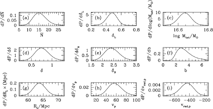
Figure 1: Probability distributions of the expected number of collapsed objects above $M_{min}$, the linear matter overdensity, $\delta_{L}$, the total mass of the SSC, $M_{tot}$, the nonlinear matter overdensity, $\delta$, the cluster overdensity, $\delta_{N}$, the cluster bias, $b$, the Lagrangian radius of the SSC, $R_{L}$, the contribution of the SSC to the peculiar velocity of the LG, $v_{p}$, and the peculiar radial velocity of the outer edge of the SSC, $v_{rad,p}$. $v_{p}$ and $v_{rad,p}$ are plotted in units of ${\rm km\,s^{-1}}$. The distributions assume $N=21$, $M_{min}=1.75\times 10^{14}\,M_{\odot}$, and $R_{E}=51\,{\rm Mpc}$.

$M_{halo}$, on the other hand, is the mass for which ePS-like prescriptions generate the mass function and corresponds roughly to the mass out to the radius within which the matter density is $180$ times the mean density. The relationship between various definitions of mass can easily be calculated (Hu & Kravtsov, 2003). Values of $M_{1625}$ underestimate those of $M_{halo}$ by $\sim 52\%$ (i.e. $M_{halo}=2.1\,M_{1625}$). We estimate errors in these masses to be about $30\%$, resulting primarily from error in the temperature measurement and intrinsic scatter in the $M-T_{X}$ and $M-L_{X}$ relations from equations (10) and (11).

Because the clusters under consideration are very massive and luminous, we ignore the effect of the cluster selection function. The flux of our dimmest cluster is bright enough to be seen even in regions where ROSAT sensitivity is slightly lower (i.e. in the $\sim 1.5\,{\rm deg}$ patch centered at (RA:DEC)$=$(199.295:-34.393)). However, absorption by the galaxy could hide a few additional clusters. On the other hand, because the core of the SSC is clearly more overdense than the region out to $50\,{\rm Mpc}$, our assumption that each cluster represents one halo may not hold there. Multiple clusters in the core may lie within a single halo (or multiple halos in the process of merging). Thus, the number of halos may be somewhat different than the $21$ we assume. Our analysis, however, is independent of the individual masses of these halos and depends only on the minimum halo mass of our sample and the total number of halos. Because the error in our mass measurements is only $30\,\%$, errors in the minimum mass can be described by additional error in the number of clusters being above a fixed threshold. In addition, we expect the variation in $N$ due to errors in $M_{halo}$ to be small. If it turns out that all of our mass estimates are systematically $30\,\%$ too high, then only two clusters below the limit would have made it into our sample undeserved. In §8, we show the dependence of our results on the exact value of $N$.

4 Shapley Overdensity

In Figure 1, we plot the distributions of several quantities calculated through the prescription outlined in §2 or derived from the resulting quantities. Panels (a)-(i) show results for the expected number of collapsed objects above $M_{min}$, the linear matter overdensity, $\delta_{L}$, the total mass of the SSC, $M_{tot}$, the nonlinear matter overdensity, $\delta$, the cluster overdensity, $\delta_{N}$, the cluster bias, $b$, the Lagrangian radius of the SSC, $R_{L}$, the contribution of the SSC to the peculiar velocity of the LG, $v_{p}$, and the peculiar radial velocity of the outer edge of the SSC, $v_{rad,p}$.

The distribution of $\bar{N}$ in panel (a) shows a mean clearly less than our assumed value of $N=21$. This is due to the $(dP/d\delta_{L})\,(d\delta_{L}/d\bar{N})$ factor in equation (7). If, in the absence of information about $N$, each value of $\bar{N}$ were equally likely, we would have $<\bar{N}>=N$. However, including the true prior probability distribution means that lower values of $\bar{N}$ are more likely.

The linear overdensity can be interpreted given the value of $\sigma=\sqrt{S}$ on the scale of the supercluster. For $R=50\,{\rm Mpc}$ ($64\,{\rm Mpc}$), $\sigma\approx 0.23$ ($0.18$). The mean linear overdensity of $\sim 0.47$ in panel (b) represents a $\sim 2.0\sigma$ ($\sim 2.6\sigma$) fluctuation in the overdensity in the region. As a sanity check, we note that the probability of a linear density as high or higher, assuming initial Gaussian fluctuations, is approximately $1/50$ ($1/200$), and there are about $[200\,{\rm Mpc}/50\,{\rm Mpc}]^{3}\sim 60$ ($[200\,{\rm Mpc}/60\,{\rm Mpc}]^{3}\sim 40$) such regions out to the distance of the SSC. So it is not unlikely that we do observe such a region within $200{\rm Mpc}$, nor is it so unlikely that the supercluster remains one of the most overdense regions out to that distance.

Our analysis gives $M_{tot}=(4.4\pm 0.44)\times 10^{16}\,M_{\odot}$ for the mass of the SSC. This is similar to the mass in the region estimated by de Filippis et al. (2005), and only a bit lower than estimates by Reisenegger et al. (2000) and Proust et al. (2006).

Panels (d)-(f) show the probability distributions of the matter overdensity, $\delta$, the cluster overdensity, $\delta_{N}$, and the cluster bias, $b$. The nonlinear overdensity distribution shows $\delta=0.76\pm 0.17$ and $\delta_{N}=2.4\pm 0.32$. Larger values of $\delta$ correspond to lower values of $\delta_{N}$ and $b$ since the number of clusters is fixed and so more matter in the region gives closer agreement between the matter and cluster densities. The bias is $b=3.5\pm 1.4$, however, the distribution is not Gaussian and is skewed toward values higher than its peak at $b\approx 1.6$. This peak value is just over $1-\sigma$ higher than the maximum of the range of $b=1.2$–$1.9$ that Kocevski & Ebeling (2006) estimated (for $\Omega_{M,0}=0.279$) by assuming that their calculation of the peculiar velocity of the LG induced by their sample is equal to the true value. We calculate only a $6\%$ chance that the bias falls into the $b=1.2$–$1.9$ range. For reference, we find that $b=1.5$ corresponds to $\delta\approx 1.2$. The discrepancy in the bias may result from differences between the clusters associated with the SCC and the entire Kocevski & Ebeling (2006) sample. The entire sample includes objects that are less intrinsically luminous (i.e. less massive) than those in the SSC.

5 Shapley Supercluster Dynamics

While we used the spherical collapse model in previous sections to calculate $R_{L}$ corresponding to $R_{E}$ for each value of $\delta_{L}$, we now look at the results from the model in detail about the dynamics of the SSC region. We describe our analysis in §5.1 and possible tests for our results in §5.2.

5.1 The Spherical Collapse Model

The evolution of the physical size $r$ of a region containing mass $M_{tot}$ is described by:

$$\frac{d^{2}s}{da^{2}}=\left(\frac{1}{H\,a}\right)^{2}\,\frac{d^{2}s}{dt^{2}}-\left(\frac{1}{a}+\frac{1}{H}\frac{dH}{da}\right)\,\frac{ds}{da}$$

$$\frac{d^{2}s}{dt^{2}}=H_{i}^{2}\,\left(-\frac{\Omega_{M,i}\,(1+\delta_{i})}{2\,s^{2}}+\Omega_{\Lambda,i}\,s\right),$$ (12)

where $M_{tot}$ is the mass in the region given by equation (9), $s=r/r_{i}$, $r$ is the evolving Eulerian size of the region, and where the evolution of the Hubble parameter is given by the Friedmann equation,

$$H=\frac{1}{a}\,\frac{da}{dt}=H_{0}\,\sqrt{\frac{\Omega_{M,0}}{a^{3}}+\Omega_{\Lambda,0}}\,.$$ (13)

The evolution of the matter and dark energy density parameters ($\Omega_{M}$ and $\Omega_{\Lambda}$, respectively) are given by

$$\Omega_{M}=(1-\Omega_{\Lambda})={\Omega_{M,0}\over\Omega_{M,0}+\Omega_{\Lambda,0}a^{3}}.$$ (14)

Subscripts “0” refer to values today, and subscripts “i” refer to initial values at $a_{i}$. We take $a_{i}=0.01$, set $s_{i}=1$ (i.e. $r=r_{i}$) and $(ds/da)_{i}=(1-\delta_{i}/3)\,(1/a_{i})$ as our initial conditions, and numerically integrate equation (12) up to $a_{f}=1/(1.0388)\approx 0.962$, corresponding to the Hubble flow redshift of A3558.

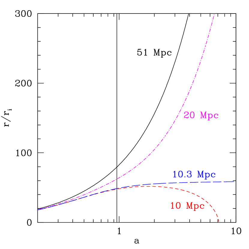
Figure 2: The evolution of spheres around the center of the SSC as a function of the scale factor, $a$, calculated from the spherical collapse model. Results are shown for radii of $51\,{\rm Mpc}$ (solid line), $20\,{\rm Mpc}$ (dot-dashed line), $10.3\,{\rm Mpc}$ (long-dashed line), and $10\,{\rm Mpc}$ (short-dashed line). Since $a=1$ today, values of $a>1$ refer to time in the future. The vertical line denotes the redshift of the SSC. The mean values of the overdensity within the radii shown have been adopted in plotting the trajectories.

In setting $(ds/da)_{i}=(1-\delta_{i}/3)\,(1/a_{i})$, as appropriate for a growing-mode perturbation, we have assumed that the region is not initially expanding with the Hubble flow as in Lokas & Hoffman (2001). The $-\delta_{i}/3$ term accounts for the peculiar velocity of the region due to its overdensity. Since we expect the $\delta_{i}$ to be small, however, the peculiar velocity term will also be small.

The probability distribution for the Lagrangian radius, $R_{L}=r_{i}/\,a_{i}$, is given in panel (g) of Figure 1. The distribution gives $R_{L}=(64\pm 2.0)\,{\rm Mpc}$, indicating that the region of the SSC deviates from the Hubble flow and collapses by only $\sim 20\%$.

The more interesting result from applying the spherical collapse model to the SSC is that the region is still expanding at a radius of $50\,{\rm Mpc}$. While not expanding as fast as the Hubble flow, the SSC has not reached turn-around. Moreover, we find that, due to the repulsive effect of the cosmological constant, the region will never reach turn-around despite its overdensity but will continue to expand forever. This can be seen in the trajectory of the $51\,{\rm Mpc}$ region plotted in Figure 2. Trajectories have also been plotted for the interior regions of the SSC (see §7).

We arrive at the peculiar radial velocity of the region by subtracting the Hubble velocity from the total expansion rate. The distribution in the peculiar radial velocity of the $50\,{\rm Mpc}$ shell, $v_{rad,p}$, is given in panel (h) of Figure 1 and gives $v_{rad,p}=(-437\pm 87)\,{\rm km\,s}^{-1}$. The minus sign indicates that the region is expanding somewhat slower than the $\approx 3600\,{\rm km\,s^{-1}}$ Hubble velocity at that radius.

5.2 Observational Tests of the Model Predictions

Our prediction for the outward velocity of the $50\,{\rm Mpc}$ shell could potentially be tested with the Tully-Fisher relation or by Type Ia supernovae (Masters et al., 2006; Springob et al., 2007; Jha et al., 2007). By determining the distance to an object of a known redshift, one may infer its peculiar velocity by subtracting off the Hubble velocity at its inferred distance. The quantity $v_{rad,p}$ is the radial peculiar velocity with respect to the center of the SSC. Thus, the peculiar velocity of the SSC itself must be accounted for when using the Tully-Fisher relation to measure $v_{rad,p}$. The latest results from Springob et al. (2007) provide a peculiar velocity for A3558, the central cluster of the SSC, of $(2980\pm 859)\,{\rm km\,s}^{-1}$. However, the error on the peculiar velocity of A3558 is too large to constrain $v_{rad,p}$ reliably. Below we explore alternative observational methods for future measurements of the predicted peculiar velocities.

The peculiar velocity of an X-ray cluster can be directly inferred from its contribution to the CMB through the kinetic Sunyaev-Zel’dovich (kSZ) effect in which CMB photons scatter off free elections moving along with the bulk velocity of the cluster. The temperature fluctuation induced in this way by a cluster is given by:

$$\frac{{\Delta}T}{T}=-\tau\,\frac{v}{c},$$ (15)

where $\tau\approx\sigma_{T}\,n_{e}\,R_{c}$ is the optical depth for Thomson scattering of the CMB by free electrons in the cluster, $\sigma_{T}$ is the Thomson cross-section, $n_{e}$ is the number density of electrons in the cluster, $R_{c}$ is its core radius, and $v$ is its peculiar velocity. The minus sign indicates that velocities away from us result in temperature decrements. Because A1644 is on the edge of the SSC (albeit the edge on the sky as opposed to along the line of sight), we use it as a test case to estimate ${{\Delta}T}/{T}$ due to $v_{rad,p}$ of a hypothetical cluster on the $50\,{\rm Mpc}$ shell and positioned along the line of sight to A3558. The radius of A1644 is $\sim 0.7\,{\rm Mpc}$, while its X-ray luminosity is $L_{X}\approx 10^{44}\,{\rm ergs\,s^{-1}}$ and its temperature is about $6\times 10^{7}$K (de Filippis et al., 2005). Accounting for the X-ray luminosity through thermal bremsstrahlung we get $n_{e}\approx 5\times 10^{-4}\,{\rm cm^{-3}}$. If the hypothetical cluster under consideration (whose properties are the same as A1644) is $50\,{\rm Mpc}$ in front of A3558 directly along the line of sight so that $v_{rad,p}$ is also along the line of sight, the CMB temperature fluctuation due to $v_{rad,p}$ would be ${{\Delta}T}/{T}\approx-2\times 10^{-6}$ with ${{\Delta}T}\approx-5\,{\rm\mu\,K}$. Because the peculiar velocity is radially inward toward the center of the SSC, if the cluster is between us and A3558, then this velocity is away from us and results in a temperature decrement.

The SSC as a whole also induces CMB signals through the kSZ effect from to its own peculiar velocity and through the Rees-Sciama effect (Rees & Sciama, 1968). For an overdensity of $\delta=0.76$, the optical depth to electron scattering through the SSC is $\tau=2.3\times 10^{-5}$. The resulting kSZ signal due to the peculiar velocity of the structure is ${{\Delta}T}/{T}\approx-2.1\times 10^{-7}$. In the Rees-Sciama effect, the evolution of the gravitational potential, $\phi=-G\,M_{tot}/R$, during the photon crossing time of the system introduces additional temperature fluctuations of order $\frac{{\Delta}T}{T}\sim\frac{\delta\phi}{c^{2}}$. If the potential becomes deeper (i.e. more negative) as a photon passes through the region, the redshift experienced by the photon on its way out of the potential well is greater than the blueshift it receives on its way in and the CMB in that direction shows a temperature decrement. However, between $z=0.051$ and $z=0.027$ (which spans the light crossing time for the SSC of $\sim[100\,{\rm Mpc}/c]$), the SSC grows from $50.47\,{\rm Mpc}$ to $51.54\,{\rm Mpc}$. For $M_{tot}=4.4\times 10^{16}\,M_{\odot}$, the change in the potential results in ${{\Delta}T}/{T}\approx 8.7\times 10^{-7}$. The kSZ and Rees-Sciama effects due to the SSC as a whole act against each other.

The predicted signal can probed by a number of upcoming CMB observatories such as Planck (http://planck.esa.int), the Arcminute Cosmology Bolometer Array Reciever (http://cosmology.berkeley.edu/group/swlh/acbar), the Atacama Pathfinder Experiment (http://www.mpifr-bonn.mpg.de/div/mm/apex), the South Pole Telescope (http://spt.uchicago.edu), and the Atacama Cosmology Telescope (ACT, http://www.physics.princeton.edu/act). With a temperature noise of $\sim 35\,{\rm\mu\,K}$ per pixel, WMAP is not sufficiently sensitive to detect this effect. On the other hand, ACT has a temperature noise of ${\delta}T\sim 5\,{\rm\mu\,K}$ per pixel and a pixel size of $3\,{\rm arcminutes^{2}}$. At a distance of $(150-50=100)\,{\rm Mpc}$, an A1644-like cluster would take up $\sim 600$ pixels, lowering the detectable level to $\sim 0.2\,{\rm\mu\,K}$. Therefore, the kSZ signal due to this cluster is, in principle, detectable with ACT at the $\sim 26\,\sigma$ level. Though additional sources of error may make this detection more challenging (Sehgal et al., 2005), the major obstacle to measuring this signal is disentangling it from the primary anisotropy that is at least an order-of-magnitude larger and has an identical spectrum. It is also important to note, that some type of distance measure from something like the Tully-Fisher relation or from Type Ia supernovae is still necessary to determine which clusters are on the $50\,{\rm Mpc}$ shell.

6 Contribution to Peculiar Velocity of the Local Group

Figure 3: The radial profile of the SSC. The number of observed clusters, $N$, the matter overdensity, $\delta$, and the amount of excess mass, $\Delta\,M_{tot}$ within $R_{E}$ as functions of $R_{E}$ are plotted in the top three panels. The bottom two panels show the peculiar velocity of the local group due to the overdensity contained within $R_{E}$ and the radial peculiar velocity of the shell with radius $R_{E}$ centered on A3558. Solid lines indicate mean values, while the dashed curves denote $1-\sigma$ bounds due to Poisson fluctuations.

Next we calaculate the contribution of the Shapley Suplercluster to the peculiar velocity of the LG, $v_{p}$, given our result for the SSC mass. The induced velocity in the linear regime is given by (Peebles, 1993)

$$v_{p}=\frac{a\,f\,H}{4\,\pi}\,\int\,\frac{\vec{y}-\vec{x}}{\left|\vec{y}-\vec{x}\right|^{3}}\,\delta(\vec{y})\,d^{3}\vec{y},$$ (16)

where $f=(a/D)\,(dD/da)\approx\Omega_{M}^{0.6}$ and $\vec{y}$ and $\vec{x}$ point from the center of the SSC to each SSC mass element and to the LG, respectively. Because we do not explore the mass distribution within the SSC, we assume a constant value of the overdensity out to $50\,{\rm Mpc}$. The distribution of values for $v_{p}$, reflecting the distribution in the SSC overdensity, is plotted in panel (i) of Figure 1. We find $v_{p}=(55\pm 13)\,{\rm km\,s}^{-1}$, only $(9.0\pm 2.1)\%$ of the $612\,{\rm km\,s}^{-1}$ peculiar velocity of the LG with respect to the CMB (Loeb & Narayan, 2007). This is much less than the value estimated by Kocevski & Ebeling (2006) of $\sim 30\%$. Even $b=1.5$ and the corresponding value of $\delta=1.2$ (see §4) produce only $v_{p}\approx 92\,{\rm km\,s^{-1}}$, but this is almost $3-\sigma$ from our mean value. Thus, we agree qualitatively with Raychaudhury et al. (1991), Reisenegger et al. (2000), and Loeb & Narayan (2007) that the SSC does not contribute very significantly to the peculiar velocity of the LG.

7 Radial Profile

The number of clusters in our sample decreases sharply with radius from the center of the SSC, and the clusters are not numerous enough to adequately sample the entire volume of the SSC. Nonetheless, we can obtain some interesting estimates about the radial distribution of the quantities we investigate by considering subsamples of clusters from Table 1 with distances from the center of the SSC within varying values of $R_{E}$.

Figure 3 shows the radial profiles we calculate for the number of observed clusters, the matter overdensity and the amount of excess mass within $R_{E}$ as functions of $R_{E}$. Also shown are the peculiar velocity of the LG due to the overdensity contained within $R_{E}$ and the radial peculiar velocity of the shell with radius $R_{E}$ centered on A3558. The plot of $N$ vs. $R_{E}$ depicts a step-like function where the value changes in discrete steps as observed clusters from the Table 1 become included in the subsample within $R_{E}$. The discreteness of the limited sample is manifested in the sharp transitions exhibited in the radial profiles of the other quantities in Figure 3. The true profiles are smooth curves that roughly follow those calculated and are bounded by the $\pm 1-\sigma$ error brackets approximately $68\%$ of the time despite the sharp transitions. The uncertainty in the values of $r$, the distance between each cluster and A3558, shown in Table 1, is not included in the errors plotted in the figure.

Since $\Delta\,M_{tot}=4\,\pi\,R_{E}^{3}\,\rho_{M}(z_{SSC})\,\delta$, the plots of $\delta$ and $\Delta\,M_{tot}$ vs. $R_{E}$ are analogous, however, they illustrate two different points. The radial profile of $\delta$ shows a roughly power-law rise in the overdensity as we move toward the center of the SSC. The supercluster becomes quite nonlinear in the region interior to $R_{E}\approx 40\,{\rm Mpc}$. The radial profile of $\Delta\,M_{tot}$, on the other hand, demonstrates that the mass only rises significantly through sharp jumps that correspond to the adding of additional clusters to the subsample. This can also be seen in the plot of $v_{p}$ vs. $R_{E}$ where the profile between jumps is extremely flat. Moreover, while the contribution to the peculiar velocity of the LG rises most rapidly between $R_{E}\approx 30\,{\rm Mpc}$ and $R_{E}\approx 45\,{\rm Mpc}$, $v_{p}$ seems to have leveled off by $R_{E}\approx 50\,{\rm Mpc}$.

The evolution of $v_{rad,p}$ with $R_{E}$ is very mild with its mean varying by only a factor of $\sim 1.5$ over the full range of $R_{E}$ shown. In addition, the $1-\sigma$ errors on $v_{rad,p}$ are large, comparable to the range over which $v_{rad,p}$ varies. However, it is clear that the general trend is toward increasingly negative values of $v_{rad,p}$ as we move toward the center of the SSC. This is what is expected from the spherical collapse model. In addition, by tracing the future of regions at different radii with the spherical collapse model (see §5.1), we determine that the SSC is only a closed system at $R_{E}\approx 10.3$ given the mean of the density probability distribution and at $R_{E}\approx 13$ if $1-\sigma$ fluctuations are considered. The mass enclosed within this radius is comparable to that of a rich X-ray cluster of $\sim 10^{15}M_{\odot}$. The trajectories of spheres with $R_{E}=10\,{\rm Mpc}$, $10.3\,{\rm Mpc}$, $20\,{\rm Mpc}$, and $51\,{\rm Mpc}$ are plotted in Figure 2. The mean values of the overdensity for each of these radii have been adopted in plotting the trajectories.

8 Robustness of Results

In §2, we showed how the matter overdensity in a region can be determined by fitting the mass function in an overdense region to the cluster mass function in the region. However, because of our limited sample, we only fit the normalization of the mass function and relied on the Barkana & Loeb (2004) hybrid model to correctly fit the slope. In this section, we investigate the robustness of our results and their dependence on our sample. In §8.1, we consider the choice of $N$ obtained from the sample, while in §8.2, we turn our attention to the slope of the mass function and ask whether different mass bins within the sample give consistent results.

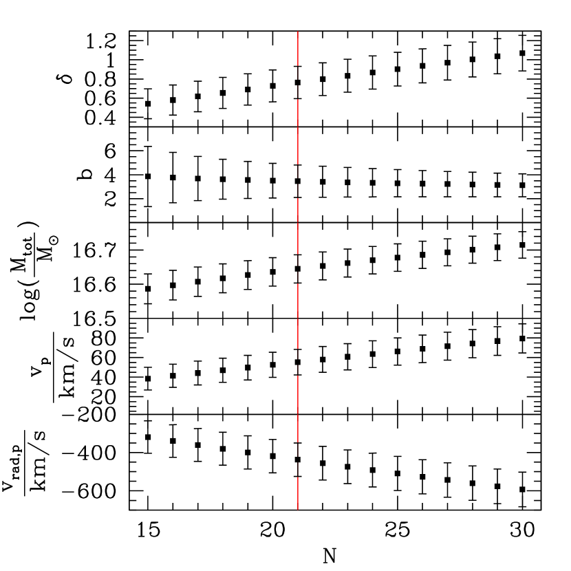
Figure 4: The dependence of the distributions for the nonlinear overdensity, $\delta$, the total mass of the SSC, $M$, the cluster bias, $b$, the contribution of the SSC to the peculiar velocity of the LG, $v_{p}$, and the radial peculiar velocity of the outer edge of the SSC, $v_{rad,p}$, on the value of $N$. The square points represent the mean values of the probability distributions, while the error bars show the $\pm 1-\sigma$ spread. The vertical line denotes $N=21$. $M_{min}=1.75\times 10^{14}\,M_{\odot}$ and $R_{E}=51\,{\rm Mpc}$ are held fixed for all values of $N$.

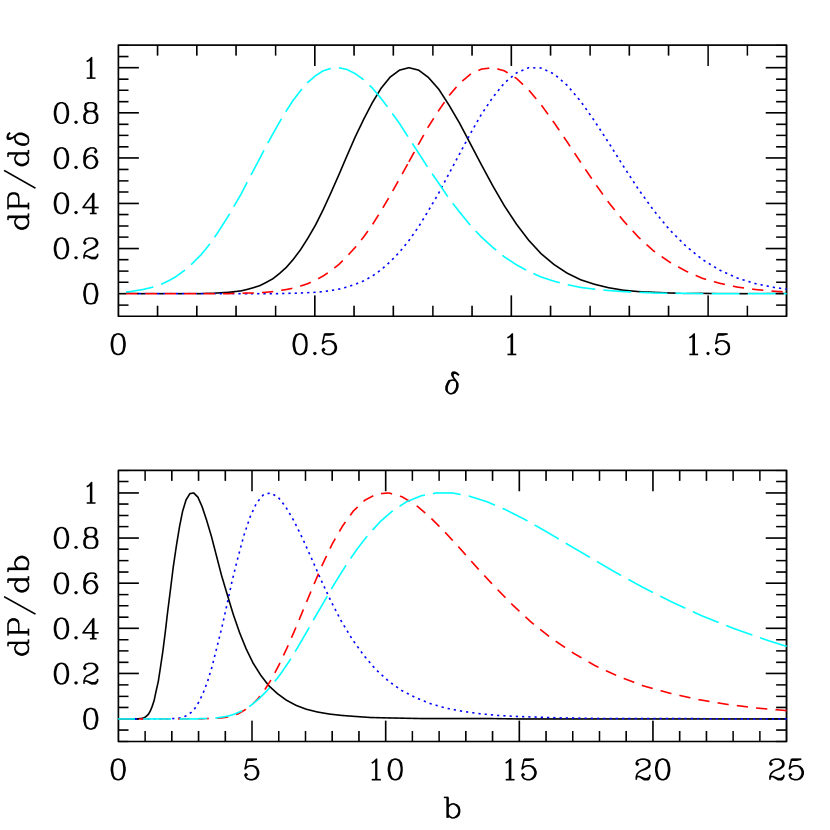
Figure 5: The probability distributions of the matter overdensity, $\delta$, (upper panel) and the cluster bias, $b$, (lower panel) obtained with four different cluster subsamples from Table 1. The solid curve shows the results from the entire sample of $21$ clusters with masses above $1.75\times 10^{14}\,M_{\odot}$ shown in Figure 1. The dotted curve shows the results obtained using the $17$ clusters with masses above $3.5\times 10^{14}\,M_{\odot}$, while the $10$ clusters with masses above $5.5\times 10^{14}\,M_{\odot}$ produced the results denoted by the dashed curve. Finally, the results denoted by the long-dashed curve were derived with only the $4$ clusters with host halo masses above $7.0\times 10^{14}\,M_{\odot}$. The size of the region was fixed at $R_{E}=51\,{\rm Mpc}$ for each distribution.

8.1 Dependence on $N$

The number of collapsed halos, their minimum mass, and their extent are the three key parameters that we extract from our cluster sample for use in our structure formation analysis. Though it is probably correct to identify the number of X-ray luminous clusters with the number of collapsed halos, the two may not be exactly equivalent. In addition, there may be undiscovered objects obscured by galactic absorption. As argued in §3, the error in the mass estimates of each halo from the cluster X-ray properties can be expressed as an additional but small error in the number of halos above a fixed threshold. The same can be said for the extent of the SSC, denoted $R_{E}$. Small errors in the physical position of a cluster with respect to the center of the SSC can be represented as clusters being falsely included or excluded in our fixed selection of $R_{E}$. We thus explore the dependence of our results on the assumed number of collapsed halos.

Figure 4 shows the mean values of $\delta$, $b$, $M$, $v_{rad,p}$, and $v_{p}$ from Figure 1, as well as the $1-\sigma$ errors for different choices of $N$. As $N$ changes, $M_{min}$ and $R_{E}$ are held fixed at the values assumed throughout this paper. The results clearly do not change much as $N$ is varied over a relatively wide range of values.

8.2 Slope of the Mass Function

Checking the fit of the mass function explicitly is equivalent to asking whether samples with higher mass thresholds give consistent results for the overdensity in the SSC. Since there are many more lower mass objects than higher mass ones, significant deviations in the number of higher mass objects may not affect the results obtained using all of the clusters. However, consistency between multiple mass bins shows that the results do not depend on the particular choices we made for our sample.

The probability distributions for the matter overdensity and the cluster bias are shown in Figure 5 calculated using each of four different mass thresholds. These distributions are not completely independent because the lower mass thresholds include all of the objects at higher mass. However, since there is a steep drop-off in the number of objects with mass, the distributions are dominated by objects near the mass threshold. All four mass thresholds give consistent results for the matter overdensity in the SSC, with the distributions clustered around $\delta\sim 0.8$, slightly higher than the mean of the $M_{min}=1.75\times 10^{14}\,M_{\odot}$ distribution. It is important to note that the mass threshold does not correlate with mean overdensity. This is just what we would expect if there is no bias in the number of objects with mass since, according to the model, a single value of the average linear matter overdensity should describe the entire mass function.

On the other hand, we do expect a correlation between the bias and the mass of the objects in the sample. The figure clearly show this correlation as the mean of each bias distribution increases with the mass threshold. This is a manifestation of the fact that more massive clusters are more strongly clustered than less massive ones.

9 Conclusions

We have used the enhanced abundance of X-ray clusters to calculate the mass in the SSC, based on the ePS-ST model (Barkana & Loeb, 2004). We constructed a sample of $21$ X-ray luminous clusters within a radius of $51\,{\rm Mpc}$ in halos with masses above $M_{min}=1.75\times 10^{14}\,M_{\odot}$. We then calculated probability distributions for the matter density contrast of the SSC region, the cluster bias for our sample, and the mass of the SSC. We demonstrated that even mild values of the overdensity in a region can result in a significant over-abundance of massive clusters. We found a mass of $M=(4.4\pm 0.44)\times 10^{16}\,M_{\odot}$ for the SSC. Our results are in good agreement with previous results (Reisenegger et al., 2000; de Filippis et al., 2005; Proust et al., 2006), though we found that the cluster bias is probably higher than that estimated by Kocevski & Ebeling (2006).

We then used the spherical collapse model to investigate the dynamics of the SSC. We found that the comoving size of the region has only collapsed by about $20\%$ from its initial value. Moreover, we concluded that the SSC is not bound at a radius of $51\,{\rm Mpc}$, despite the significant mass in the region. The repulsive effect of the cosmological constant provides the extra push against gravity that will keep the region from ever collapsing. The outer shell is moving radially away from the center with a velocity only $(437\pm 87)\,{\rm km\,s}^{-1}$ slower than the $\approx 3600\,{\rm km\,s^{-1}}$ Hubble velocity at that radius. This prediction could be tested with better Tully-Fisher data from SSC galaxies, or future CMB observations.

We also calculated the contribution of the SSC to the peculiar velocity of the LG, $v_{p}=(55\pm 13)\,{\rm km\,s}^{-1}$. This value amounts to only $(9.0\pm 2.1)\%$ of the LG peculiar motion, much smaller than a recent estimate by Kocevski & Ebeling (2006) and more in agreement with Raychaudhury et al. (1991), Reisenegger et al. (2000), and Loeb & Narayan (2007).

Despite the uncertainty in investigating the interior of the SSC using smaller subsamples of cluster, exploring the radial profiles of $\delta$, $v_{p}$, and $v_{rad,p}$ indicated convergence, i.e. that we have included all of the mass in the region in excess of the universal average that contributes to the peculiar velocity of the LG. Moreover, while the $50\,{\rm Mpc}$ region as a whole is only mildly nonlinear, the interior of the SSC becomes highly nonlinear. The excess mass becomes enough to bind the sphere with radius only $\sim 10\,{\rm Mpc}$.

Finally, we showed that our results are robust to errors in our input parameters and the mass threshold of our cluster sample. Subsamples of clusters with different mass thresholds give consistent results for the overdensity in the region and demonstrate an expected increase in bias with mass.

10 Acknowledgements

We would like to thank C. Jones, K. Masters, R. Narayan, and especially A. Vikhlinin for useful discussions. Thanks also to D. Kocevski for his list of X-ray clusters in the SSC. JM acknowledges support from a National Science Foundation Graduate Research Fellowship. This research was supported in part by Harvard University funds.

References

- Bahcall et al. (2004) Bahcall N. A., Hao L., Bode P., Dong F., 2004, ApJ, 603, 1
- Barkana & Loeb (2004) Barkana R., Loeb A., 2004, ApJ, 609, 474
- Bond et al. (1991) Bond J. R., Cole S., Efstathiou G., Kaiser N., 1991, ApJ, 379, 440
- de Filippis et al. (2005) de Filippis E., Schindler S., Erben T., 2005, A&A, 444, 387
- Ebeling et al. (2002) Ebeling H., Mullis C. R., Tully R. B., 2002, ApJ, 580, 774
- Ettori et al. (1997) Ettori S., Fabian A. C., White D. A., 1997, MNRAS, 289, 787
- Evrard et al. (2002) Evrard A. E., MacFarland T. J., Couchman H. M. P., Colberg J. M., Yoshida N., White S. D. M., Jenkins A., Frenk C. S., Pearce F. R., Peacock J. A., Thomas P. A., 2002, ApJ, 573, 7
- Fabian (1991) Fabian A. C., 1991, MNRAS, 253, 29P
- Haines et al. (2006) Haines C. P., Merluzzi P., Mercurio A., Gargiulo A., Krusanova N., Busarello G., La Barbera F., Capaccioli M., 2006, MNRAS, 371, 55
- Hu & Kravtsov (2003) Hu W., Kravtsov A. V., 2003, ApJ, 584, 702
- Jha et al. (2007) Jha S., Riess A. G., Kirshner R. P., 2007, ApJ, 659, 122
- Kocevski & Ebeling (2006) Kocevski D. D., Ebeling H., 2006, ApJ, 645, 1043
- Komatsu et al. (2008) Komatsu E., Dunkley J., Nolta M. R., Bennett C. L., Gold B., Hinshaw G., Jarosik N., Larson D., Limon M., Page L., Spergel D. N., Halpern M., Hill R. S., Kogut A., Meyer S. S., Tucker G. S., Weiland J. L., Wollack E., Wright E. L., 2008, ArXiv e-prints, 803
- Loeb & Narayan (2007) Loeb A., Narayan R., 2007, ArXiv e-prints, 711
- Lokas & Hoffman (2001) Lokas E. L., Hoffman Y., 2001, ArXiv Astrophysics e-prints
- Masters et al. (2006) Masters K. L., Springob C. M., Haynes M. P., Giovanelli R., 2006, ApJ, 653, 861
- Mo & White (1996) Mo H. J., White S. D. M., 1996, MNRAS, 282, 347
- Muñoz & Loeb (2008) Muñoz J. A., Loeb A., 2008, MNRAS, 385, 2175
- Peebles (1993) Peebles P. J. E., 1993, Principles of physical cosmology. Princeton Series in Physics, Princeton, NJ: Princeton University Press, —c1993
- Proust et al. (2006) Proust D., Quintana H., Carrasco E. R., Reisenegger A., Slezak E., Muriel H., Dünner R., Sodré Jr. L., Drinkwater M. J., Parker Q. A., Ragone C. J., 2006, A&A, 447, 133
- Quintana et al. (1995) Quintana H., Ramirez A., Melnick J., Raychaudhury S., Slezak E., 1995, AJ, 110, 463
- Raychaudhury et al. (1991) Raychaudhury S., Fabian A. C., Edge A. C., Jones C., Forman W., 1991, MNRAS, 248, 101
- Rees & Sciama (1968) Rees M. J., Sciama D. W., 1968, Nat, 217, 511
- Reisenegger et al. (2000) Reisenegger A., Quintana H., Carrasco E. R., Maze J., 2000, AJ, 120, 523
- Sehgal et al. (2005) Sehgal N., Kosowsky A., Holder G., 2005, ApJ, 635, 22
- Sheth et al. (2001) Sheth R. K., Mo H. J., Tormen G., 2001, MNRAS, 323, 1
- Sheth & Tormen (1999) Sheth R. K., Tormen G., 1999, MNRAS, 308, 119
- Springob et al. (2007) Springob C. M., Masters K. L., Haynes M. P., Giovanelli R., Marinoni C., 2007, ApJS, 172, 599
- Vikhlinin (2008) Vikhlinin A., 2008, ArXiv Astrophysics e-prints
- Zhang et al. (2008) Zhang J., Ma C.-P., Fakhouri O., 2008, ArXiv e-prints, 801