Reanalysis of two eclipsing binaries: EE Aqr and Z Vul

Abstract

We study the radial-velocity and light curves of the two eclipsing binaries $EE$ $Aqr$ and $Z$ $Vul$. Using the latest version of the Wilson & Van Hamme (2003) model, absolute parameters for the systems are determined. We find that $EE$ $Aqr$ and $Z$ $Vul$ are near-contact and semi-detached systems, respectively. The primary component of $EE$ $Aqr$ fills about 96% of its ’Roche lobe’, while its secondary one appears close to completely filling this limiting volume. In a similar way, we find fill-out proportions of about 72 and 100% of these volumes for the primary and secondary components of $Z$ $Vul$ respectively. We compare our results with those of previous authors.

Keywords Variable stars- Binaries- Eclipsing binary

1 Introduction

Eclipsing binary stars studies often involve the combination of photometric (light curve) and spectroscopic (mainly, radial velocity curve) data. The analysis of the light-velocity curves enable astronomers to obtain absolute physical parameters describing the system and its components. The physical parameters derived from the photometric and spectroscopic data can help to improve our understanding of physical processes in stars. In view of the importance of $EB$-$EA$ type binary stars in the problem of mass exchange in binaries and in the theory of their evolution, the study of these systems play an important role in finding of the complex initial phases of stellar evolution. In order to understand the physical nature of $EB$ and $EA$ type binaries, two candidates, $EE$ $Aqr$ and $Z$ $Vul$, were selected based on the following criteria: a) the shape of the light curve, b) their photoelectric measurements are not enough and also somewhat the analysis results derived by the previous authors appear to differ from each other. The first, we state their history in literature and then describe our solution method.

1.1 $EE$ $Aqr$

The binary system $EE$ $Aqr$ (HD213863, BD-$20^{\circ}$6454, SAO 191236, $\alpha_{2000}=22^{h}34^{m}41^{s}.87,$ $\delta_{2000}=19^{\circ}51^{\prime}34^{\prime\prime}$) was discovered to be variable by Strohmeier & Knigge (1960). Strohmeier et al. (1962) derived its eclipsing behavior with a orbital period of $0.51$ $d$ and classified it as an Algol (EA) type eclipsing binary. Later, the photoelectric observations were obtained by Williamon (1974), Padalia (1979) and Covino et al. (1988). Williamon (1974) who showed the light curves to be more like that of $\beta$ Lyrae (EB) type with a period of $0.5089951$ $d$ and analyzed these using the method of Russell & Merrill (1952). Thus preliminary photometric orbital parameters of the system were derived. Slightly different orbital parameters were determined by Padalia (1979) for the system using the same method. Russo & Sollazzo (1982) found many inconsistencies in applying the Russell and Merrill (1952) method of solution. Therefore they reanalyzed both $V$ light curves of Williamon (1974) and Padalia (1979) using the Wilson & Devinney (1971) model. They obtained the same results for both light curves while the Russell-Merrill model does not. They found a solution as a semi-detached system. The system has also been studied spectroscopically by Hilditch & King (1988), from which radial-velocities were measured for both components by means of the cross-correlation code VCROSS. The first simultaneous solution of photometric and radial-velocity curves was performed by Covino et al. (1990) based on the Wilson & Devinney (1971) model. Their solution indicated that $EE$ $Aqr$ might be a contact configuration not yet in thermal equilibrium. From 1990 to now, no analysis of light curves and new photometric observations has been reported.

The period variations of the system has studied by Srivastava (1987) who found irregular changes of the order of $\pm 10^{-6}$ $d$ and many observations of the times of minima (Mallama (1980), Covino et al. (1988), Deeg et al.(2003)) so far.

The spectral classes of the components of $EE$ $Aqr$ were given as F0 (Williamon (1974)), FV+A (Padalia (1979)), A8V+(K3-K4)(Russo & Sollazzo (1982)).

1.2 $Z$ $Vul$

The variability of $Z$ $Vul$ (HD181987, $\alpha_{2000}=19^{h}\;21^{m}\\ 39^{s}.11,$ $\delta_{2000}=25^{\circ}34^{\prime}29^{\prime\prime}.45$) was discovered to be an eclipsing binary by Herschel (It has been reported by Astbury, 1909). Plaskett (1920), Petrie (1950), Roman (1956), Popper (1957b) and Cester et al. (1977) determined the spectral type of the components as B3, B4+B6, B5V+A, B3-4V+A2-3III and B2V+A1III respectively. The first researches on the system presented its eclipsing behavior with a orbital period slightly less than $2.5$ $d$ and classified it as an Algol (EA) type eclipsing binary. Cester et al. (1977) analyzed Broglia’s photometric observations (1964) using the $WINK$ program (Wood, 1972) and determined slightly different masses, radii and luminosities for the system with those found in the literature. They found a solution as a semi-detached system.

Peters (1994) presented the first IUE observations to investigate the effect of the cross-section and temperature of the primary on the mass transfer and mass loss in the system. They found that the primary involve with weak winds, originating from the gas stream will strike the primary instead of forming an accretion disk. The lack of H-alpha emission in system supports this proposition.

The first results from far-UV observations obtained by Peters & Polidan (1997) about the nature of the circum stellar material in the system. Their observations showed no infalling from a gas stream. So it is consistent with this fact that the system is sufficiently close and can not establish a disk.

It is recognized that depend on applying present models, we can obtained the same or different results of analyzing light-velocity curves and thus it follows an low or high understanding of stellar evolution. Therefor it is need to research a tool for a better comprehension of the binaries structure and evolutive stage.

In this study the authors adopted the more realistic close binary model based on the Roche model. In order to obtain accurate solutions in this situation, the light curves were analyzed by means of the latest the Wilson’s computer code. The computing code used was developed by the Wilson & Van Hamme code (2003)(here after WV) to determine the parameters of the system. We selected it as our analysis research tool both for its intrinsic virtues and because of some improvements in comparison with earlier code (Wilson & Divinney, 1971). The fourth revision (2003) is improved for example based on Kurucz’s new atmospheres, log g as a parameter (allowing for handling giants, sub-giants, etc., in addition to main sequence stars) so that temperature ranges vary according to log g together with 19 abundances (relative to the sun). Hence we felt it useful to reanalyze these systems and get the most reliable elements with the model of WV, which was developed especially to handel close systems and compare our finding with results of the previous authors.

All the data we analyze in the paper are taken from the literature so that these data appeared to be free from any peculiarities reported by the previous researches. We consider photometric observations of Williamon (1974) (here after WI) and spectroscopic observations of Hilditch & King (1988) (here after HK) for $EE$ $Aqr$ and the photometric observations of Broglia (1964) (here after BR) and spectroscopic observations of Popper (1957b) (here after PO) for $Z$ $Vul$.

The present paper is organized as follows. The assumptions are described in section 2. Photometric solutions of light curves is given in section 3. Spectroscopic solutions of radial velocities curves in section 4. Absolute elements for the primary and secondary components in section 5 and in section 6, we give conclusion.

2 Assumptions

The latest 2003 version of the Wilson program was applied for photometric and spectroscopic solutions. The method assumes the star surfaces to be equipotential and uses a set of curve-dependent or curve-independent parameters that can be adjusted by $LC$ and $DC$ programs: the orbital inclination $i$, surface potentials $\Omega_{1,2}$, the mean surface effective temperatures $T_{1,2}$, the mass ratio $q=m_{2}/m_{1}$, the bandpass luminosities $L_{1,2}$, the wavelength-specific limb darkening coefficients $x_{1,2}$, the bolometric limb darkening coefficients $x_{1,2}(bol)$, the bolometric gravity darkening exponents g_1,2 and the bolometric albedos $A_{1,2}$. Throughout this paper, the subscripts 1 and 2 refer to the primary (hotter) and the secondary (cooler) components, respectively.

For both components of the systems, we used bolometric linear, logarithmic and square root law and the best result was obtained for bolometric logaritmic limb darkening law of Klinglesmith & Sobieski (1970) of the form:

$$I=I_{\circ}(1-x+x\cos\theta-y\cos\theta\ln(\cos\theta)),$$ (1)

where the limb darkening coefficients $x$ and $y$ for both components were fixed to their theoretical values, interpolated using Van Hamme’s (1993) formula which have tabulated in tables 1 and 2.

The gravity darkening exponent from Lucy (1967) and the bolometric albedos from Rucinski (2001) were chosen for convective envelopes ($g=0.32,A=0.5$) and for radiative envelopes ($g=1.0,A=1.0$), which are agreement with the final surface temperature. In order to reduce the number of free parameters these parameters were kept constant during all the iterations. Also it is assumed that this binary system has zero orbital eccentricity ($e=0.0$) and that its rotational and orbital spins are synchronous ($F_{1}=F_{2}=1.0$). Also black body models are employed, and we assume that there is no third light ($l_{3}=0.0$) for both systems.

Table 1 : The limb darkening coefficients for $EE$ $Aqr$

Parameters	Filter B	Filter U	Filter V
$x_{1}(bol)$	0.640	0.640	0.640
$y_{1}(bol)$	0.255	0.255	0.255
$y_{2}(bol)$	0.153	0.153	0.153
$x_{1}$	0.690	0.795	0.788
$x_{2}$	0.800	0.802	0.834
$y_{1}$	0.291	0.328	0.279
$y_{2}$	-0.014	-0.411	-0.189

Table 2 : The limb darkening coefficients for $Z$ $Vul$

Parameters	Filter B	Filter U	Filter V
$x_{1}(bol)$	0.762	0.762	0.762
$x_{2}(bol)$	0.703	0.703	0.703
$y_{1}(bol)$	0.090	0.090	0.090
$y_{2}(bol)$	0.072	0.072	0.072
$x_{1}$	0.434	0.482	0.509
$x_{2}$	0.584	0.615	0.682
$y_{1}$	0.233	0.228	0.275
$y_{2}$	0.290	0.249	0.336

3 Photometric Solutions

Using the photometric data from the WI and BR, we derived the final elements of the systems. Before beginning the analysis, we have chosen some parameters of the systems using the spectroscopic and photometric information as a starting input values.

Initially, the light curve program (LC) was implemented in mode 2 with no third light (based on the spectroscopic observations, HK and PO) corresponding to detached configuration by choosing i, $T_{2}$ (while the temperature of the primary component was assumed from spectroscopic or color data), $\Omega_{1,2}$ and $L_{1}$ as adjustable parameters in UBV filters. The symmetry between the maximums in the light curves indicate the lack of star spots on the components. After a few runs of the LC program an initial set of values was employed as input parameters for the DC program. After a few runs with the differential correction program, we could not obtain the values of the physical parameters with less error, thus making change to mode 5 so that expected from the earlier workers. By several iterations of the $LC$ and $DC$ programs and adjusting the parameters $i,T_{2},\Omega_{1}$ and $L_{1}$ for each filter, finally the solution evolved into a nearcontact configuration for $EE$ $Aqr$ and semi-detached one for $Z$ $Vul$. The results of light curve solutions with the final elements are given in Tables 3 and 4. The theoretical light curves computed with these results are shown in Figures 1 and 2. The agreement between the observed (solid circles) and the theoretical light curves (continuous lines) is quite good.

Table 3 : The photometric parameters of $EE$ $Aqr$

Parameters	This work	This work	This work	Williamon	Padalia	Russo and	Hilditch	Covino et	Covino et
	B Filter	U Filter	V Filter	(1974)	(1979)	Sollazzo	and King	al. (1990)	al. (1990)
	(Johnson)	(Johnson)	(Johnson)			(1982)	(1988)	$BVRI$	$BVRI$&$RV$
$i$	80.5074	81.3365	78.9509	73.71	74.00	76.0	80.5	80.0	80.2
	$\pm$ 0.2975	$\pm$ 0.4360	$\pm$ 0.2379
$q$	0.32	0.32	0.32	0.503	0.500	0.4	0.32	0.332	0.327
	fixed	fixed	fixed
$T_{1}$	7060	7060	7060	8000	8000	8000	7060	7230	7227
	fixed	fixed	fixed
$T_{2}$	4200	3952	4173	4340	4365	4440	4395	4240	4233
	$\pm$ 116	$\pm$ 252	$\pm$ 85
$\Omega_{1}$	2.6178	2.6141	2.6030	3.002	3.003	2.78		2.619	2.568
	$\pm$ 0.0118	$\pm$ 0.0106	$\pm$ 0.0116
$\Omega_{2}$	2.5100	2.5100	2.5100	2.882	2.875	2.68		2.538	2.561
$L_{1}/(L_{1}+L_{2})$	0.9832	0.9950	0.9716	0.966	0.964	0.951	0.952	0.959
$L_{2}/(L_{1}+L_{2})$	0.0168	0.0050	0.0284	0.034	0.036	0.049	0.048	0.041
log g1(CGS)	4.33	4.33	4.33
log g2(CGS)	4.24	4.24	4.24
$r_{1}(pole)$	0.4303	0.4310	0.4330	0.394	0.394		0.434	0.43	0.44
	$\pm$ 0.0021	$\pm$ 0.0019	$\pm$ 0.0021
$r_{1}(point)$	0.5121	0.5139	0.5194	0.469	0.467			0.52	0.54
	$\pm$ 0.0056	$\pm$ 0.0051	$\pm$ 0.0059
$r_{1}(side)$	0.4568	0.4577	0.4603	0.415	0.414			0.46	0.47
	$\pm$ 0.0027	$\pm$ 0.0025	$\pm$ 0.0027
$r_{1}(back)$	0.4765	0.4775	0.4806	0.437	0.435			0.48	0.49
	$\pm$ 0.0033	$\pm$ 0.0030	$\pm$ 0.0033
$r_{2}(pole)$	0.2659	0.2659	0.2659	0.300	0.299		0.262	0.27	0.26
	$\pm$ 0.0025	$\pm$ 0.0017	$\pm$ 0.0032
$r_{2}(point)$	0.3853	0.3853	0.3853	0.406	0.405			0.36	0.33
	$\pm$ 0.0121	$\pm$ 0.0080	$\pm$ 0.0153
$r_{2}(side)$	0.2769	0.2769	0.2769	0.313	0.312			0.28	0.27
	$\pm$ 0.0027	$\pm$ 0.0018	$\pm$ 0.0034
$r_{2}(back)$	0.3096	0.3096	0.3096	0.345	0.345			0.31	0.30
	$\pm$ 0.0027	$\pm$ 0.0018	$\pm$ 0.0034
$\Omega_{in}$	2.5100	2.5100	2.5100
$\Omega_{out}$	2.3114	2.3114	2.3114
$\Sigma$ $\omega(o-c)^{2}$	0.0172	0.0234	0.0156

Table 4 : The photometric parameters of $Z$ $Vul$

Parameters	This work	This work	This work	Popper	Cester et al. (1977)
	B Filter	U Filter	V Filter	(1957b)	B Filter	U Filter	V Filter
	(Johnson)	(Johnson)	(Johnson)		(Johnson)	(Johnson)	(Johnson)
$i$	88.6106	88.5185	88.6478	88	88	88.5	88.9
	$\pm$ 0.0666	$\pm$ 0.0453	$\pm$ 0.0772
$q$	0.43	0.43	0.43		0.43	0.43	0.43
	fixed	fixed	fixed
$T_{1}$	19840	19840	19840		19850	19850	19840
	fixed	fixed	fixed
$T_{2}$	10909	9882	10810		9000	10290	9410
	$\pm$ 25	$\pm$ 32	$\pm$ 27
$\Omega_{1}$	3.7975	3.8512	3.7434
	$\pm$ 0.0106	$\pm$ 0.0083	$\pm$ 0.0119
$\Omega_{2}$	2.7387	2.7387	2.7387
$L_{1}/(L_{1}+L_{2})$	0.8151	0.8869	0.7889		0.962	0.930	0.954
$L_{2}/(L_{1}+L_{2})$	0.1849	0.1131	0.2111		0.038	0.070	0.046
log g1(CGS)	3.87	3.89	3.86
log g2(CGS)	3.49	3.49	3.49
$r_{1}(pole)$	0.2954	0.2908	0.3002
	$\pm$ 0.0009	$\pm$ 0.0007	$\pm$ 0.0011
$r_{1}(point)$	0.3086	0.3031	0.3144
	$\pm$ 0.0011	$\pm$ 0.0008	$\pm$ 0.0013
$r_{1}(side)$	0.3011	0.2962	0.3063
	$\pm$ 0.0010	$\pm$ 0.0007	$\pm$ 0.0012
$r_{1}(back)$	0.3058	0.3006	0.3113
	$\pm$ 0.0011	$\pm$ 0.0008	$\pm$ 0.0012
$r_{2}(pole)$	0.2881	0.2881	0.2881
	$\pm$ 0.0004	$\pm$ 0.0004	$\pm$ 0.0005
$r_{2}(point)$	0.4142	0.4142	0.4142
	$\pm$ 0.0018	$\pm$ 0.0016	$\pm$ 0.0021
$r_{2}(side)$	0.3004	0.3004	0.3004
	$\pm$ 0.0004	$\pm$ 0.0004	$\pm$ 0.0005
$r_{2}(back)$	0.3330	0.3330	0.3330
	$\pm$ 0.0004	$\pm$ 0.0004	$\pm$ 0.0005
$\Omega_{in}$	2.7387	2.7387	2.7387
$\Omega_{out}$	2.4781	2.4781	2.4781
$\Sigma$ $\omega(o-c)^{2}$	0.0039	0.0057	0.0031

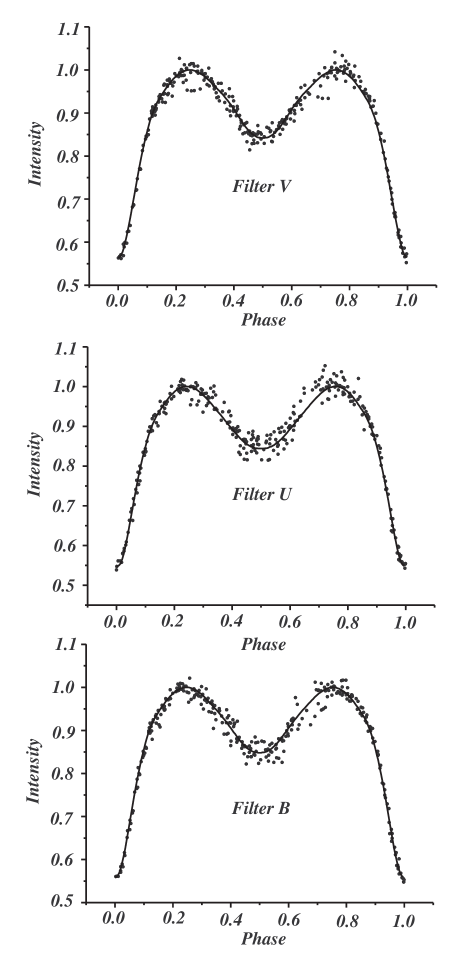
Fig. 1 : The observed and theoretical light curves of $EE$ $Aqr$. Solid circles show the observed data and the theoretical light curves are shown by continuous lines.

Fig. 2 : The observed and theoretical light curves of $Z$ $Vul$. Solid circles show the observed data and the theoretical light curves are shown by continuous lines.

4 Spectroscopic Solutions

Using the radial-velocity data from HK and PO, we derived the orbital elements of the systems. Adjustable parameters were the following: the orbital semi-major axis $a$, the radial velocity of the binary system center of mass $V_{\gamma}$. The results are given in table 5. Using the final elements of the objects, the theoretical radial-velocity curves are shown in Figure 3. The agreement between the observed (solid circles) and the theoretical radial-velocity curves (continuous lines) is quite good.

Table 5 : The spectroscopic parameters

Parameters	$EE$ $Aqr$	$Z$ $Vul$
$V_{\gamma}(Km/s)$	-1.6786	-22.7690
	$\pm$ 0.6520	$\pm$ 0.3952
$a(R_{\odot})$	4.1240	15.8411
	$\pm$ 0.0188	$\pm$ 0.0454

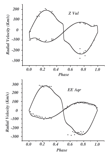
Fig. 3 : The observed and theoretical radial-velocity curves of $EE$ $Aqr$ and $Z$ $Vul$. Solid circles show the observed data and the theoretical radial-velocity curves are shown by continuous lines.

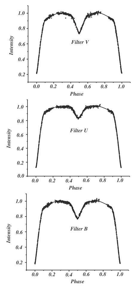
Fig. 4 : The observed and theoretical radial-velocity curves of AV Del. Solid circles show the observed data and the theoretical radial-velocity curve is shown by continuous lines.

5 Absolute Elements

Using the obtained results of the light and radial-velocity curves, we calculate the absolute parameters of the systems. The results are listed in tables 6 and 7. We determine the absolute dimensions using the following formulae:

$$M_{1}/M_{\odot}=f_{1}(M_{1},M_{2},i)(1+q)^{2}/\sin^{3}i,$$ (2)

$$f_{1}(M_{1},M_{2},i)=(M_{2}\sin i)^{3}/(M_{1}+M_{2})^{2},$$ (3)

$$M_{2}/M_{\odot}=q(M_{1}/M_{\odot}),$$ (4)

$$R_{1,2}/R_{\odot}=4.207(M_{1,2}/M_{\odot}(1+q)P^{2}(days))^{1/3}r(side),$$ (5)

$$L_{1,2}/L_{\odot}=(R_{1,2}/R_{\odot})^{2}(T_{1,2}/T_{\odot})^{4},$$ (6)

$$\rho_{1,2}/\rho_{\odot}=(0.01344M_{1,2})/[(M_{1}+M_{2})P^{2}r^{3}_{1,2}],$$ (7)

$$(M_{bol})_{1,2}=42.36-10\log T_{1,2}-5\log(R_{1,2}/R_{\odot}).$$ (8)

Table 6 : The absolute elements of the binary system $EE$ $Aqr$

Parameters	This Work	This Work	This Work	Russo and	Hilditch and	Covino et
	Filter B	Filter U	Filter V	Sollazzo	King (1988)	al. (1990)
	(Johnson)	(Johnson)	(Johnson)	(1982)
$M_{1}/M_{\odot}$	2.761	2.761	2.761	1.9	2.2	2.14
$M_{2}/M_{\odot}$	0.883	0.883	0.883	0.95	0.71	0.70
$L_{1}/L_{\odot}$	6.55	6.55	6.55	9.16		7.8
$L_{2}/L_{\odot}$	0.32	0.25	0.32	0.47		0.33
$R_{1}/R_{\odot}$	1.88	1.88	1.88	1.58	1.75	1.79
$R_{2}/R_{\odot}$	1.18	1.18	1.18	1.21	1.07	1.06
$\rho_{1}/\rho_{\odot}$	0.4123	0.4099	0.4030
$\rho_{2}/\rho_{\odot}$	0.5922	0.5922	0.5922
$M_{1}(bol)$	2.55	2.55	2.53
$M_{2}(bol)$	5.82	6.08	5.85
$f_{1}(M_{1},M_{2},i)$	0.0498	0.0501	0.0490

Table 7 : The absolute elements of the binary system $Z$ $Vul$

Parameters	This Work	This Work	This Work	Popper (1957b)	Cester et al. (1977)
	Filter B	Filter U	Filter V
	(Johnson)	(Johnson)	(Johnson)
$M_{1}/M_{\odot}$	6.209	6.209	6.209	5.4	5.4
$M_{2}/M_{\odot}$	2.670	2.670	2.670	2.3	2.3
$L_{1}/L_{\odot}$	2631.37	2543.85	2720.37	1850	2818
$L_{2}/L_{\odot}$	252.75	170.21	243.75	175	162
$R_{1}/R_{\odot}$	4.77	4.69	4.85	4.7	4.5
$R_{2}/R_{\odot}$	4.89	4.89	4.89	4.7	4.6
$\rho_{1}/\rho_{\odot}$	0.0571	0.0600	0.0543
$\rho_{2}/\rho_{\odot}$	0.0247	0.0247	0.0247
$M_{1}(bol)$	-3.96	-3.93	-4.00	-3.5
$M_{2}(bol)$	-1.42	-0.99	-1.38	-1.0
$f_{1}(M_{1},M_{2},i)$	0.2412	0.2412	0.2412

6 Conclusion

Comparing the new photometric-spectroscopic solutions of the systems with those of given in literature, the present authors can get following conclusions:

1-In our study, we may conclude that the systems are near-contact and semi-detached for $EE$ $Aqr$ and $Z$ $Vul$ respectively. The fillout for the components can be calculated from the following formula:

$$fillout_{1,2}=\frac{\Omega_{in}}{\Omega_{1,2}}\times 100.$$ (9)

Also from the following formulae we calculate $K_{1,2}$ and $a_{1,2}\sin i$ for each of the systems:

$$K_{1,2}=\frac{2\pi a_{1,2}\sin i}{P},$$ (10)

$$a_{1}\sin i=[\frac{GP^{2}f_{1}(M_{1},M_{2},i)}{4\pi^{2}}]^{\frac{1}{3}},$$ (11)

$$a_{2}\sin i=\frac{a_{1}\sin i}{q}.$$ (12)

The derived values of the parameters are given in tables 8 and 9. According to our results, $EE$ $Aqr$ is a near-contact system which the primary and secondary components filling are almost $96\pm 1$ and $100$ percent of their respective critical Roche lobes. Also $Z$ $Vul$ is a semi-detached system that the primary and secondary components filling are almost $72\pm 1$ and $100$ percent of their respective critical Roche lobes. The fillout percentage was not accurately determined in previous workers ($86\pm 3$ and $94\pm 3$ percent according to HK for the primary and secondary components of $EE$ $Aqr$, respectively; no information for ones of $Z$ $Vul$). It seems that fillout obtained from our solutions is appropriate for highly evolved system.

2- According to our synthetic light curves, $EE$ $Aqr$ is $\beta$-Lyrae type and $Z$ $Vul$ is an $Algol$ type system. Also according to the obtained parameters of the systems, we have drawn the configuration of the components using the Binary Maker 2.0 (BradStreet, 1993) software, which are shown in figures 4 and 5.

3- The new values of the velocity amplitudes and the gama velocity differ only slightly from earlier researches.

4- The absolute elements of both components determine the evolutionary state of the systems. Entering the results in the mass-luminosity (M-L), $M_{bol}$-mass (M-M), mass-radius (M-R) and H-R diagrams (the diagrams are displayed in figures 6 and 7, it appears that $EE$ $Aqr$ contains two main-sequence stars with F2IV+K4III spectral type while the primary of $Z$ $Vul$ is still a main-sequence object, and the secondary component is on its way to the giant stage with B2V+B9V spectral type for the primary and secondary respectively (according to tables of Straizys & Kuriliene, 1981). The results are tabulated in table 10 and compared with the results of the pervious authors.

Table 8 : Other elements of the binary system $EE$ $Aqr$

Parameters	This Work	This Work	This Work	Hilditch and
	Filter B	Filter U	Filter V	King (1988)
	(Johnson)	(Johnson)	(Johnson)
$a_{1}\sin i$	0.9876	0.9899	0.9827	0.92
$a_{2}\sin i$	3.0880	3.0951	3.0728	2.85
$K_{1}(Km/s)$	98.2403	98.4678	97.7579	91.3
$K_{2}(Km/s)$	307.1819	307.8929	305.6733	284
$fillout$ $1$(%)	95.882	96.020	96.428	86
$fillout$ $2$(%)	100.000	100.000	100.000	94

Table 9 : Other elements of the binary system $Z$ $Vul$

Parameters	This Work	This Work	This Work	Plaskett (1920)	Popper (1957b)
	Filter B	Filter U	Filter V
	(Johnson)	(Johnson)	(Johnson)
$a_{1}\sin i$	4.7716	4.7714	4.7717
$a_{2}\sin i$	11.0963	11.0958	11.0964
$K_{1}(Km/s)$	98.4167	98.4127	98.4182	96.4	89.8
$K_{2}(Km/s)$	228.8649	228.8557	228.8685	213.7	219.7
$fillout$ $1$(%)	72.118	71.112	73.161
$fillout$ $2$(%)	100.000	100.000	100.000

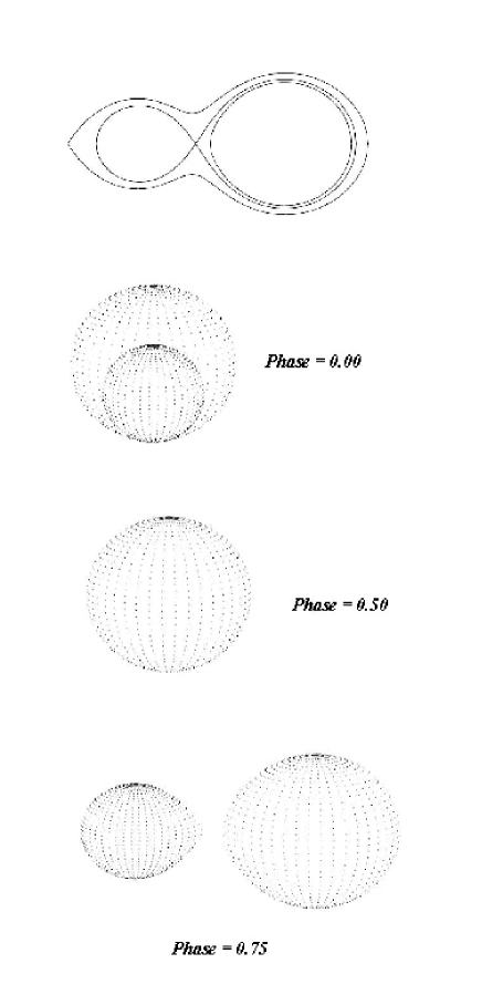
Fig. 5 : Configuration of binary system $EE$ $Aqr$

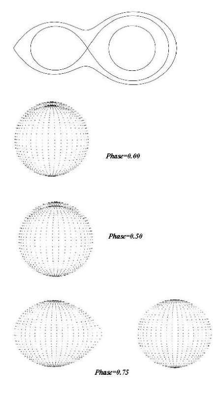
Fig. 6 : Configuration of binary system $Z$ $Vul$

Table 10 : Spectral type of $EE$ $Aqr$ and $Z$ $Vul$

Star	This work	Williamon	Padalia	Russo and	Plaskett	Petrie	Roman	Poper	Cester et al.
		(1974)	(1979)	Sollazzo	(1920)	(1950)	(1956)	(1957b)	(1977)
				(1982)
$EE$ $Aqr$ (primary)	F2 IV	F0	F V	A8 V
$EE$ $Aqr$ (secondary)	K4 III		A	K3-K4
$Z$ $Vul$ (primary)	B2 V				B3	B4	B5 V	B3-4 V	B2 V
$Z$ $Vul$ (secondary)	B9 V				B3	B6	A	A2-3 III	A1 III

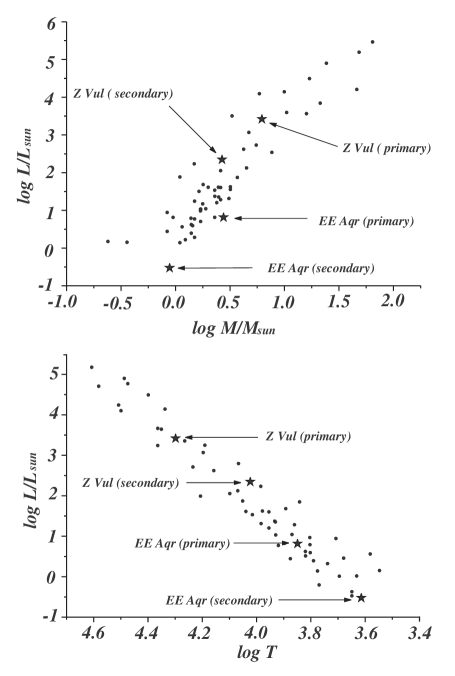
Fig. 7 : M-L and H-R diagram. The location of components are shown with star sign.

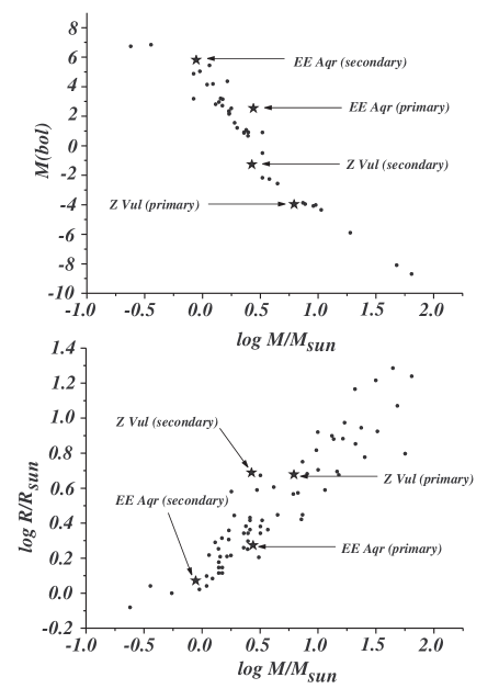
Fig. 8 : M-M and M-R diagram. The location of components are shown with star sign.

Acknowledgements We wish to very thank professor Bahram Khalesseh for his useful comments and discussion at various stage of the work. Also we would like to thank the referee for their comments and suggestions.

References

- (1) Astbury, T.H.: AN. 182, 389 (1909)
- (2) Bradstreet, D.H.: Light curve modeling of eclipsing binary stars, Springer-Verlage, P. 151 (1993)
- (3) Broglia, P.: J. Obs. 47, 99 (1964)
- (4) Cester, B., Fedel, B., Giuricin, G., Mardirossian, F., Pucillo, M.: Astron. Astrophys. 61, 469 (1977)
- (5) Covino, E., Barone, F., Milano, L., Russo, G., Sarna, M.J.: Mon. Not. R. Astron. Soc. 246, 472 (1990)
- (6) Covino, E., Milano, L., de Martino, D., Vittone, A.A.: Astron. Astrophys. Suppl. Ser. 73, 437 (1988)
- (7) Deeg, H.J., Doyle, L.R., Bejar, V.J.S., Blue, J.E., Huver, S.: IBVS. 5470, 1 (2003)
- (8) Hilditch, R.W., King, D.J.: Mon. Not. R. Astron. Soc. 232, 147 (1988)
- (9) Klinglesmith, D.A., Sobieski, S.: Astron. J. 75, 175 (1970)
- (10) Lucy, L.B.: Zeit. Fur Astrophysic. 65, 89 (1967)
- (11) Mallama, A.D.: Astrophys. J. Suppl. Ser. 44, 241 (1980)
- (12) Padalia, T.D.: Astrophys. Space Sci. 62, 477 (1979)
- (13) Peters, G.J.: iue. prop., 4819 (1994)
- (14) Peters, G.J., Polidan, R.S.: American Astron. Soc. 190, 4202 (1997)
- (15) Petrie, R.M.: Pub. Dom. Ap. Obs. Victoria. 8, 319 (1950)
- (16) Plaskett, J.S.: Pub. Dom. Ap. Obs. Victoria. 1, 251 (1920)
- (17) Popper, D.M.: Astrophys. J. 126, 53 (1957b)
- (18) Roman, N.G.: Astrophys. J. 123, 246 (1956)
- (19) Rucinski, S.M.: Astronomical J., 122, 1007 (2001)
- (20) Russell, H.N., Merrill, J.E.: Contrib. Princeton Univ. Observatory. No.26 (1952)
- (21) Russo, G., Sollazzo, C.: Astr. Astrophys. 107, 197 (1982)
- (22) Strayzis, V., Kuriliene, G.: Astrophys. Space Sci. 80, 353 (1981)
- (23) Srivastava, R.K.: Astrophys. Space Sci. 129, 221 (1987)
- (24) Strohmeier, W., Knigge, R., Ott, H.: Veroff. Remeis-Sternw. Bamberg. V. No. 5, 2 (1962)
- (25) Strohmeier, W., Knigge, R.: Veroff. Remeis-Sternw. Bamberg. V. No. 5, 2 (1960)
- (26) Van Hamme, W.: Astron. J. 106, 2096 (1993)
- (27) Williamon, R.M.: Astrophys. J. 79, 1093 (1974)
- (28) Wilson, R.E., Devinney, E.J.: Astrophys. J. 166, 605 (1971)
- (29) Wilson, R.E., Van Hamme, W.: Computing Binary Star Observables (2003)
- (30) Wood, D.B.: A Computer Program for Modelling Non-Spherical Eclipsing Binary Systems, Goddard Space Flight Center, Greenbelt, Maryland, USA (1972)