Physical replicas and the Bose-glass in cold atomic gases

Abstract

We study cold atomic gases in a disorder potential and analyze the correlations between different systems subjected to the same disorder landscape. Such independent copies with the same disorder landscape are known as replicas. While in general these are not accessible experimentally in condensed matter systems, they can be realized using standard tools for controlling cold atomic gases in an optical lattice. Of special interest is the overlap function which represents a natural order parameter for disordered systems and is a correlation function between the atoms of two independent replicas with the same disorder. We demonstrate an efficient measurement scheme for the determination of this disorder-induced correlation function. As an application, we focus on the disordered Bose-Hubbard model and determine the overlap function within perturbation theory and a numerical analysis. We find that the measurement of the overlap function allows for the identification of the Bose-glass phase in certain parameter regimes.

I Introduction

The interplay between disorder and interaction gives rise to a plethora of fundamental phenomena in condensed matter systems. The most predominant examples include spin glasses Binder and Young (1986); Mézard et al. (1987); Young (1998), the superconducting-to-insulator transition in thin superconducting films Finkel’Stein (1994); Fisher (1990), and localization phenomena in fermionic systems such as weak localization and the metal-insulator transition Lee and Ramakrishnan (1985). While the nature of order in spin glasses and its theoretical description is still highly debated Parisi (1979); Mézard et al. (1984); Bray and Moore (1986); Fisher and Huse (1986); Binder and Young (1986); Huse and Fisher (1987); Newman and Stein (1996); Krzakala and Martin (2000); Palassini and Young (2000), a substantial contribution to the understanding of bosons in a disordered medium has been provided by work on the disordered Bose-Hubbard model introduced by Fisher et al. Fisher et al. (1989). The disordered Bose-Hubbard model has recently attracted considerable attention due to its potential realization with cold atomic gases in an optical lattice Damski et al. (2003); Sanpera et al. (2004); Roth and Burnett (2003a, b); Bloch et al. (2007); Lewenstein et al. (2007); Jaksch and Zoller (2004).

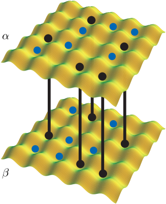
Figure 1: (Colour online) Schematic representation of the implementation of disorder replicas with the cold atomic gases toolbox: Two planes $\alpha$ and $\beta$ with equal disorder realisations, illustrated here for the case of a disorder landscape introduced using a second particle species (black dots), in which additional probe atoms (blue/lighter dots) evolve. The planes can be combined to measure correlation functions, such as the Edwards-Anderson overlap function.

A general challenge in the description of glass phases in disordered media is the absence of a simple order parameter distinguishing the different ground states. This problem becomes evident in the disordered Bose-Hubbard model where the phase diagram is determined by the competition between a superfluid phase, the Mott-insulator, and a Bose-glass phase. While the superfluid phase exhibits a finite condensate fraction and is characterized by off-diagonal long-range order, the Bose glass is only distinguished from the incompressible Mott-insulator by a vanishing excitation gap and a finite compressibility. However, in experiments on cold atomic gases the excitation gap and the compressibility are difficult to determine accurately and are also obscured by the finite harmonic trapping potential. The challenge is therefore to develop measurement schemes allowing for the experimental determination of these observables or to develop new observables to characterize the glass phase. While inaccessible in “real materials,” the Edwards-Anderson order parameter Edwards and Anderson (1975); Binder and Young (1986) is commonly studied analytically and measured numerically to quantify the “order” in a disordered system. It can be expressed as the correlation between independently evolving systems with the same disorder landscape (so-called replicas), or as a correlation of the same system at different temporal measurements. Because the latter depends on an extra variable (temporal measurement window) it is advantageous to study two replicas of the system with the same disorder. Thus, the measurement of this order parameter requires the preparation of several samples with exactly the same disorder landscape, and the subsequent measurement of correlations between these.

We demonstrate that such a procedure is feasible in cold atomic gases allowing one to gain access to characteristic properties of disordered systems naturally hidden in condensed matter systems. The basic idea is to focus on cold atomic gases in an optical lattice: along one direction, the optical lattice is very strong and divides the system into independent two-dimensional (2D) planes Stöferle et al. (2004); Sebby-Strabley et al. (2006); Fölling et al. (2007); Spielman et al. (2007). In addition, the system is subjected to a disorder potential and we are interested in the situation where in each plane the same disorder landscape is realized (see figure 1). Although the atoms in different planes are decoupled, the presence of the same disorder landscape within each plane induces a correlation between the different realizations: this correlation is of special interest in the replica theory of spin glasses and allows one to measure the overlap function, a characteristic property of spin glasses. Furthermore, we show that this correlation function is accessible in experiments on cold gases: The main idea is to quench the motion of the atoms by a strong optical lattice, and combine the different planes into a single one. Subsequently, the particle number occupation within each well carries the information about the correlation function. The possibility for the accurate determination of the particle number within each well of an optical lattice has recently been demonstrated experimentally for the superfluid-Mott-insulator quantum phase transition Campbell et al. (2006).

Note that this measurement scheme for the overlap between system with the same disorder can be applied to any disordered one- or two-dimensional system realized with cold atomic gases in an optical lattice. Of special interest is the realization of spin glasses and their study in the quantum regime. As an application, we focus here on the disordered Bose-Hubbard model and calculate the overlap function analytically in different regimes and compare it with one-dimensional numerical simulations. We find that the overlap function $q$ exhibits a sharp crossover from the Mott-insulating phase with $q\approx 0$ com (a) to the Bose-glass phase with $q\approx p(1-p)$, with $p\in(0,1)$, and thus makes it possible to distinguish the two phases. Because the superfluid phase can be detected via the interference peaks in a time-of-flight measurement, we propose that this novel measurement scheme for the overlap function can be used for a qualitative experimental verification of the phase diagram for the disordered Bose-Hubbard model.

Different implementations of disorder or quasi-disorder in cold atomic gases have been discussed and experimentally realized. Several groups attempted to search for traces of Anderson localization and the interplay of disorder-nonlinear interactions in Bose-Einstein condensates (BECs). The first experiments Lye et al. (2005); Fort et al. (2005); Clément et al. (2005, 2006); Schulte et al. (2005) were performed with laser speckles that had a disorder correlation length larger than the condensate healing length. Localisation effects were thus washed out by interactions. As an alternative, superlattice techniques—which are combinations of several optical potentials with incommensurable spatial periods—were used to produce quasi-disordered potentials with short correlations. This approach allowed the observation of some signatures of the Bose glass by the Florence group Fallani et al. (2007). Only very recently the Palaiseau group has managed to create speckle potentials on the sub-micron scale and directly observe Anderson localisations effects in a BEC released in a one-dimensional waveguide Billy et al. (2008) based on the theoretical predictions of Sanchez-Palencia et al. (2007, 2008). The Florence group reported observations of localisations phenomena in quasi-disordered potentials in BEC of K³⁹, which allows for complete control of the strength atomic interactions using Feshbach resonances Roati et al. (2008). It is worth noting that experimental attempts for local addressability in an optical lattice also offer the possibility to create disorder with correlation lengths comparable to the lattice spacing Lee et al. (2007); Gorshkov et al. (2008). Mixtures of cold gases, on the other hand, provide an alternative approach for the realization of disorder by quenching the motion of one species by a strong optical lattice, which then provides local impurities for the second species Vignolo et al. (2003); Gavish and Castin (2005). While production of 2D planes with equal disorder realisations follows naturally if the disorder is implemented with laser speckles, we also show how such a system can be realized in the case of disorder induced by a mixture of atomic gases.

In section II, we start with a detailed description of the disordered Bose-Hubbard model and the different disorder realizations. After a short review of the phase diagram of the disordered Bose-Hubbard model, we provide the definition of the overlap function $q$ characterizing the disorder-induced correlations between independent realizations of the system. In section III, we describe in detail the preparation of the system and the subsequent measurement scheme for the overlap function. In section IV, we determine the overlap for the disordered Bose-Hubbard model via perturbation theory for physically-relevant limits and compare the result with numerical simulations of the one-dimensional system. Details of the calculations are presented in the appendices.

II Bose-Hubbard model with disorder

Cold atomic gases subjected to an optical lattice are well described by the Bose-Hubbard model Jaksch et al. (1998); Schulte et al. (2005)

$$H=-J\sum_{\langle ij\rangle}b_{i}^{{\dagger}}b_{j}+\frac{U}{2}\sum_{i}n_{i}(n_{i}-1)-\sum_{i}(\mu-\Delta_{i})n_{i},$$ (1)

with $b^{{\dagger}}_{i}$ ($b_{i}$) the bosonic creation (annihilation) operator and $n_{i}=b_{i}^{{\dagger}}b_{i}$ the particle number operator at the lattice site $i$. The first term describes the kinetic energy of the atoms with hopping energy $J$ between nearest-neighbour sites, the second term accounts for the onsite interaction between the atoms, and the third term describes the disorder potential with random-site off-sets $\Delta_{i}$ of the chemical potential $\mu$.

The disorder potential $\{\Delta_{i}\}$ can be generated via different methods Lye et al. (2005); Fort et al. (2005); Clément et al. (2005); Fallani et al. (2007); Vignolo et al. (2003); Gavish and Castin (2005) and is determined by a probability distribution $P(\delta)$ describing the probability of having an onsite shift with strength $\delta$. The mean square of the disorder distribution

$$\Delta^{2}=\int d\delta\>\delta^{2}P(\delta)$$ (2)

gives rise to a characteristic energy scale $\Delta$ of the disorder potential (note that the mean energy shift of the disorder potential is absorbed in the definition of the chemical potential). In addition, the disorder potential is characterized by a correlation length. Here, we are interested in short-range disorder with the disorder in different wells independent of each other. The probability distribution $P(\delta)$ and its correlation length depend on the source of the disorder potential, which varies depending on the microscopic implementation in cold gases. The most promising possibilities in order to produce disorder with short correlation length involve the use of laser speckle patterns and mixtures of different cold atomic gases. While first experiments with laser speckles had a disorder correlation length larger than the lattice spacing Lye et al. (2005); Fort et al. (2005), experimental efforts towards local addressability in an optical lattice also offer the possibility for the creation of disorder with a correlation length comparable to the lattice spacing, as well as Gaussian probability distributions Lee et al. (2007); Gorshkov et al. (2008). Alternatively, a disorder potential can also be created in mixtures of cold atomic gases in optical lattices Günter et al. (2006); Ospelkaus et al. (2006) by quenching the motion of one species. Then, the disorder correlation length is of the order of the Wannier function, which can be smaller than the lattice spacing due to the strong lattice that quenches the motion of the disorder species, whilst the probability distribution becomes bimodal with $\Delta_{i}=\pm\Delta$; here we are primarily interested in such a short ranged disorder with $\Delta_{i}$ being independent in the different wells. Note that both Gaussian disorder, as well as bimodal disorder generally give rise to different physical phenomena in glass physics and thus both are interesting in their own right.

The zero-temperature phase diagram of the Hamiltonian  (1) was first studied by Fisher et al. Fisher et al. (1989) where three different phases were discussed: the superfluid, the Mott-insulator, and the Bose-glass phases. In the two-dimensional regime of interest here, the superfluid phase appears for large hopping energies $J\gtrsim U,\Delta$ and is characterized by off-diagonal (quasi) long-range order (finite superfluid condensate) and a linear excitation spectrum giving rise to a finite compressibility. On the other hand, for dominating interaction energies $U\gg\Delta,J$ the ground state corresponds to an incompressible Mott-insulator phase with an excitation gap and a commensurate filling factor, i.e., the averaged particle number in a single well $\langle n_{i}\rangle\in\mathrm{N}$ is an integer. While the quantum phase transition from the superfluid to the Mott-insulator has been experimentally identified Greiner et al. (2002), the disorder potential gives rise to an additional Bose-glass phase characterized by a vanishing excitation gap and finite compressibility; see figure 2 for a sketch of the phase diagram. The details of the phase diagram have been studied via analytical methods in the regime of Anderson localization Gavish and Castin (2005); Kuhn et al. (2005); de Martino et al. (2005); Lugan et al. (2007a) and in other regimes via numerical methods such as quantum Monte Carlo Scalettar et al. (1991), density matrix renormalization group (DMRG) Rapsch et al. (1999), dynamical mean-field theory Byczuk et al. (2005), and analytical methods Yukalov et al. (2007); Krutitsky et al. (2008). Furthermore, recent interests focused also on the appearance of alternative phases for different disorder types in the Bose-Hubbard model, e.g., off-diagonal disorder giving rise to a Mott-glass phase Sengupta and Haas (2007) while random onsite interactions can give rise to a Lifshits glass Lugan et al. (2007b).

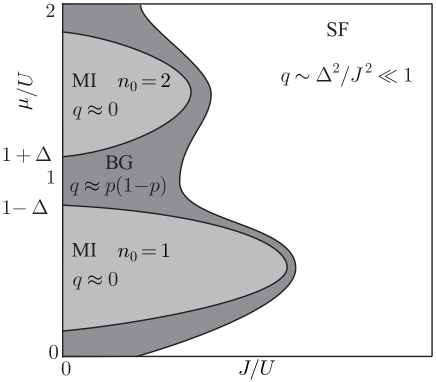
Figure 2: Sketch of the phase diagram for the disordered Bose-Hubbard model: the Mott-insulator (MI) appears for integer filling and the overlap function $q$ vanishes for small hopping $J/U\ll 1$, while in the Bose-glass phase (BG) the overlap function approaches a finite value $q=p(1-p)$ with $p\in(0,1)$ characterizing the bimodal disorder distribution (see section IV). Consequently a measurement of the overlap allows for a clear distinction between the Bose-glass and the Mott-insulator phase in this regime. In turn, the superfluid phase (SF) is characterized by off-diagonal long-range order resulting in coherence peaks in a time of flight experiment.

The superfluid phase in the absence of disorder is experimentally identified via a measurement of the coherence peaks characterizing the condensate fraction, while the transition to a Mott-insulating phase is characterized by the disappearance of these interference patterns and as well as a change in the behaviour of excitations Greiner et al. (2002); Stöferle et al. (2004). However, the identification of the Bose-glass phase in the presence of disorder requires an additional observable allowing for the distinction between the Mott-insulator and the Bose-glass, where the condensate fraction vanishes. Such an additional property is known from spin-glass theory as the Edwards-Anderson order parameter Edwards and Anderson (1975); Binder and Young (1986) which appears as an order parameter in the mean-field theory on spin glasses Parisi (1983). In the present situation with a disordered Bose-Hubbard model, its generalization leads to

$$q_{\scriptscriptstyle EA}=[\left(\langle n_{i}\rangle-n\right)^{2}]_{av}=[\langle n_{i}\rangle^{2}]_{av}-\left([\langle n_{i}\rangle]_{av}\right)^{2}\,,$$ (3)

where $n=[\langle n\rangle_{i}]_{av}$ denotes the mean particle density in the sample. It is important to note the different averages involved in the definition of the order parameter $q_{\scriptscriptstyle EA}$: for a fixed disorder realization, the average $\langle...\rangle$ denotes the thermodynamic average over the ground state of the system, while $[...]_{av}$ describes the disorder average over different disorder realizations. While the experimental determination of this quantity in the Bose-Hubbard model requires an exact state tomography of the system for each lattice site, a simpler and alternative route is obtained by preparing two systems with the same disorder landscape and measuring the correlations between these two decoupled systems: the remaining correlation is disorder induced and disappears for weak disorder. This so-called overlap function $q$ between the two systems realized with the same disorder landscape takes the form

$$q=[\langle n_{i}^{\alpha}\rangle\langle n_{i}^{\beta}\rangle]_{av}-[\langle n_{i}^{\alpha}\rangle]_{av}[\langle n_{i}^{\beta}\rangle]_{av}$$ (4)

and where $\alpha$ and $\beta$ describe the two different systems with the same disorder. This definition follows in close analogy of the mean-field order parameter in the replica theory of spin glasses Parisi (1983).

III Measurement of the overlap function

In this section we outline the key process of this work, i.e., the basic experimental procedure by which physical replicas can be prepared and used to measure the overlap function $q$ defined in (4). This consists of three essential steps: (1) initial preparation of disorder replicas, (2) introduction of probe atoms and (3) the measurement process, involving recombination of the replicas and spectroscopy to measure the overlap itself. At no stage do we assume individual addressability of lattice sites, but rather consider global operations and the measurement of global quantities.

III.1 Initial preparation of disorder replicas

We consider a situation in which atoms are confined to a three-dimensional optical lattice, which is particularly deep along the $z$-direction, so that an array of planes with 2D lattice potentials are formed in the $x$–$y$ plane, with no tunneling between the planes. Each of these 2D planes of the potential can be divided into two subplanes, again along the $z$-direction, by adding a superlattice of half the original period which can be controllably switched on and off Sebby-Strabley et al. (2006); Fölling et al. (2007). The resulting two subplanes then constitute our replicas, and our goal is that these pieces should have the same disorder realisation.

In the case of disorder generated optically (using, e.g., speckle patterns) the different layers exhibit the same disorder landscape for a suitable orientation of the lasers. However, for a disorder induced by a second species, the replicas must be produced in several steps. We start with a two-species mixture in the undivided plane. A fast ramping up of the optical lattice depth within the plane for the disorder species results in a Poissonian distribution of particles in the lattice. The next step is then a filtering procedure removing singly-occupied sites and keeping only doubly-occupied and unoccupied sites (which are distributed randomly). Such a filtering procedure has been achieved in recent experiments where atoms are combined to Feshbach molecules, and atoms remaining unpaired are removed from the system using a combination of microwave and optical fields that is energy-selective based on the molecular binding energy Winkler et al. (2006). Finally, the superlattice is applied adiabatically providing a double-layer structure, where exactly one atom of the disorder species is transferred to each of the two subplanes. The result is two planes with a random distribution of atoms of the “disorder species,” with an exact copy in each subplane, i.e., a replica of the random disorder pattern. This is illustrated in figure 1.

Interactions between atoms of a probe species and the disorder species can now be adiabatically increased, or the probe species otherwise adiabatically introduced to the system (e.g., using spin-dependent lattices or superlattices). This results in two replicas of the same system, which we label $\alpha$ and $\beta$, with atoms in each replica evolving independently according to their system Hamiltonian in the same disorder potential. We again reiterate that the superlattice separating the replicas should be deep, so that there is no tunnelling between the replicas. The only correlations between the two should thus be determined by the identical disorder realisations.

III.2 Measurement process

To measure the overlap $q$ as given by (4) we need to compute correlation functions that compare the state of probe atoms in the two replicas $\alpha$ and $\beta$. In each case, the correlation functions can be computed if we measure the joint probability distribution for occupation numbers in the two replicas (this is discussed in detail below). In particular, we need to determine the joint probability of having $n$ particles in layer $\alpha$ and $m$ particles in layer $\beta$ at a given lattice site, denoted by $p_{nm}$, and the probability of having $n$ particles in layer $\alpha$, $\beta$ at a given lattice site, denoted by $p_{n}^{\alpha,\beta}$ (both depicted in figure 3). We thus first freeze the state in each replica by ramping the lattice suddenly to deeper values in all three directions, so that tunnelling no longer occurs. We can then measure the different possible configurations of particles occupying individual lattice sites in the layers $\alpha$ and $\beta$ (see figures 3–5).

This is done in two steps: First, the layers are combined so that at each site each initial eigenstate involving different occupation numbers in the two replicas becomes a superposition of degenerate states involving the total number of atoms spread over motional states in a single well (see figure 4, section III.2.2 below). The final state is, of course, strongly dependent on the combination process, as well as the initial state before the combination of the layers. However, we need only determine the fraction of lattice sites with a total of $n$ particles, denoted $p_{n}$, which is unchanged provided that the lattice is deep within each plane, to prevent tunnelling of atoms. The relative frequency with which each final configuration $p_{n}$ occurs can then be measured based on the different spectroscopic energy shifts arising from different numbers of atoms in the final well, and different distributions of atoms over the motional states (see figure 5, section III.2.3 below). This involves weak coupling of atoms to an auxiliary internal state, similar to that performed in Campbell et al. (2006). We show that the set of possible final states given an initial configuration can be distinguished spectroscopically from the set of states corresponding to initial configurations giving different contributions to $p_{n}$, and thus we can reconstruct the original joint probability distribution $p_{nm}$ prior to combining the layers. The reduced probabilities $p_{n}^{\alpha,\beta}$ can be determined from similar spectroscopy without first combining the layers, allowing the full overlap function $q$ to be constructed. Below we give further details of each step in this procedure.

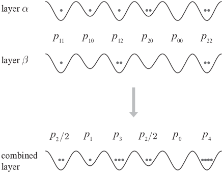
Figure 3: A sample system illustrating the required joint and combined system probabilities involved in the measurement scheme before and after combining the two layers respectively. Top: The individual layers $\alpha$ and $\beta$ and the corresponding joint probability $p_{nm}$ at each site. Bottom: Combined layer and the corresponding combined system probability $p_{n}$ at each site. Note that this is only a guide, because after combining the layers the particles are spread across multiple motional states (not depicted).

III.2.1 Quantities that need to be measured

We need to measure two quantities to determine the overlap $q$, namely $[\langle\hat{q}_{1}\rangle]_{av}$, where

$$\hat{q}_{1}=\frac{1}{L}\sum_{i}n_{i}^{\alpha}n_{i}^{\beta}$$ (5)

with $\alpha\neq\beta$ and $L$ is the total number of lattice sites, corresponding to the density-density correlations between the two layers, and $[\langle\hat{q}^{\alpha}_{2}\rangle]_{av}$, $[\langle\hat{q}^{\beta}_{2}\rangle]_{av}$, where

$$\hat{q}_{2}^{\alpha,\beta}=\frac{1}{L}\sum_{i}n_{i}^{\alpha,\beta},$$ (6)

corresponding to the average density of each layer. Then we can express

$$q=[\langle\hat{q}_{1}\rangle]_{av}-[\langle\hat{q}^{\alpha}_{2}\rangle]_{av}[\langle\hat{q}^{\beta}_{2}\rangle]_{av}.$$ (7)

The disorder average should be performed by repeated measurements of the quantum average for different realisations of the disorder com (b). In general, one can expect that a measurement on $n_{i}$ and $n_{j}$ for large separation between sites $i$ and $j$ is independent of each other, and consequently the summation over lattice sites automatically performs a statistical quantum average com (c). In the following, we are interested in small filling factors such that lattice sites with three or more particles are rare and can be neglected in all three phases of the system.

First we focus on measurement of $[\langle\hat{q}_{2}^{\alpha}\rangle]_{av}[\langle\hat{q}_{2}^{\beta}\rangle]_{av}$, i.e., the second term of the overlap in (4). If the layers are prepared as discussed above, the symmetry $(1/L)\sum_{i}\langle n_{i}^{\alpha}\rangle=(1/L)\sum_{i}\langle n_{i}^{\beta}\rangle$ is preserved and thus we can measure the average over two replicas, $[\langle\hat{q}_{2}\rangle]^{2}$ where com (d)

$$\hat{q}_{2}=\frac{1}{2}(\hat{q}_{2}^{\alpha}+\hat{q}_{2}^{\beta})=\frac{1}{2L}\sum_{i}(n_{i}^{\alpha}+n_{i}^{\beta}).$$ (8)

For the average density we obtain:

$$\langle\hat{q}_{2}\rangle=\frac{1}{2L}\sum_{i}\langle n_{i}^{\alpha}\rangle+\langle n_{i}^{\beta}\rangle=\frac{1}{2}\sum_{n}n(p_{n}^{\alpha}+p_{n}^{\beta}),$$ (9)

where $p_{n}^{\alpha,\beta}=N_{n}^{\alpha,\beta}/L$ with $N_{n}^{\alpha,\beta}$ the number of sites with $n$ particles in layers $\alpha,\beta$, and thus

$$\langle\hat{q}_{2}\rangle=\frac{1}{2}(p_{1}^{\alpha}+p_{1}^{\beta}+2p_{2}^{\alpha}+2p_{2}^{\beta}).$$ (10)

Next we consider the measurement of $[\langle\hat{q}_{1}\rangle]$ i.e., the first part of the overlap in (4). In this case the density-density correlations can be expressed as

$$\frac{1}{L}\sum_{i}\langle n_{i}^{\alpha}n_{i}^{\beta}\rangle=\sum_{n}nmp_{nm},$$ (11)

where $p_{nm}=N_{nm}/L$ with $N_{nm}$ the total number of sites with $n$ particles in layer $\alpha$ and $m$ particles in layer $\beta$, and thus, keeping terms up to two particles in total over the replicas at a given site

$$\langle\hat{q}_{1}\rangle=\frac{1}{L}\sum_{i}\langle n_{i}^{\alpha}n_{i}^{\beta}\rangle=p_{11}+2(p_{12}+p_{21})+4p_{22}.$$ (12)

Now consider $p_{n}=N_{n}/L$, with $N_{n}$ the total number of particles from both layers, which can be measured by combining both layers (described in detail in section III.2.2) and subsequently applying a similar scheme to the one presented in Campbell et al. (2006) (described in detail in section III.2.3). Using the following equations that relate both $p_{n}$ and $p_{n}^{\alpha,\beta}$ to $p_{nm}$

$$\begin{array}[]{llllll}p_{1}&=&p_{01}+p_{10}&p_{1}^{\alpha}&=&p_{10}+p_{12}+p_{11},\\ p_{2}&=&p_{20}+p_{02}+p_{11}&p_{1}^{\beta}&=&p_{01}+p_{21}+p_{11},\\ p_{3}&=&p_{12}+p_{21}&p_{2}^{\alpha}&=&p_{20}+p_{21}+p_{22},\\ p_{4}&=&p_{22}&p_{2}^{\beta}&=&p_{02}+p_{12}+p_{22},\end{array}$$

we can show that $p_{11}=\frac{1}{2}(p_{1}^{\alpha}+p_{1}^{\beta}-p_{1}-p_{3})$ which in conjunction with $p_{3}=p_{12}+p_{21}$ and $p_{4}=p_{22}$ gives all necessary terms. Then,  (12) simplifies to

$$\langle\hat{q}_{1}\rangle=\frac{1}{2}(p_{1}^{\alpha}+p_{1}^{\beta}-p_{1})+\frac{3}{2}p_{3}+4p_{4}.$$ (13)

Finally, note that $\hat{q}_{2}$ as given in  (10), can also be expressed as $\langle\hat{q}_{2}\rangle=\frac{1}{2}\sum_{n}np_{n}$.

In the following two sections we show how to measure these conditional probabilities by combining the two replicas together, and performing spectroscopy where a single atom is coupled to a different internal state. In section III.2.2 we describe the process of combining the two layers into a single one whilst in section III.2.3 we describe a similar scheme to the one presented in Campbell et al. (2006) that can be used to distinguish different occupation numbers.

III.2.2 Combining Layers

We now describe in more detail the process of combining the two layers into a single one and determine the resulting joint state for the different possible initial configurations. The combination of the layers is achieved by lowering the potential barrier that separates both layers (switching off the superlattice). Specifically, we now determine the final (after completely lowering the barrier) state for each of the different initial configurations of particles (prior to lowering the barrier).

After the superlattice is removed and layers are combined, the system is described by the Hamiltonian

$$H_{\rm\scriptscriptstyle comb} = \sum_{k\in\{0,1\}}\left[\epsilon_{k}n_{k}+\frac{U_{kk}}{2}n_{k}(n_{k}-1)\right]+2U_{01}n_{0}n_{1},$$

where $U_{kl}=2\omega_{\perp}a\int dz|w_{k}(z)|^{2}|w_{l}(z)|^{2}$, with $a$ the scattering length, $\omega_{\perp}$ the transverse trapping frequency, $w_{k}(z)$ the Wannier functions for band $k$, and $\epsilon_{k}$ the band energy ($k,l\in\{0,1\}$). The expression for $U_{kl}$ is a special case of the general 3D expression

$$U=\frac{4\pi\hbar^{2}a}{m}\int dxdydz|w_{0}(x)|^{4}|w_{0}(y)|^{4}|w_{k}(z)|^{2}|w_{l}(z)|^{2},$$

where $w_{0}(x)$ and $w_{0}(y)$ are the Wannier functions for the lowest motional state in the 2D replica plane $(x,y)$, with the additional assumption of an isotropic and deep lattice potential in the replica plane characterized by the frequency $\omega_{\perp}$.

States which are initially nondegenerate will evolve adiabatically to the corresponding eigenstate of the Hamiltonian in (III.2.2), provided the barrier is lowered slowly with respect to the energy separation between the (nondegenerate) eigenstates. However, we note that some of the initial states are doubly degenerate due to the equal single particle energies in the two layers. Thus when the barrier is lowered these degenerate states become coupled to each other (because the single particle states change time dependently) and the final state will evolve into a process-dependent superposition of the different corresponding eigenstates of the Hamiltonian in (III.2.2). However, this poses no problem for our measurement scheme since the states that are initially degenerate contribute equally to the probabilities we are trying to measure. Moreover, for a given initial configuration it is not necessary to know the full final state, in fact it is sufficient to know only the possible corresponding final eigenstates of the Hamiltonian in (III.2.2) (with the same number of particles as the initial configuration) that contribute to the final state. Figure 4 depicts all the different possible states before and after combining the layers for up to a maximum of four particles in total.

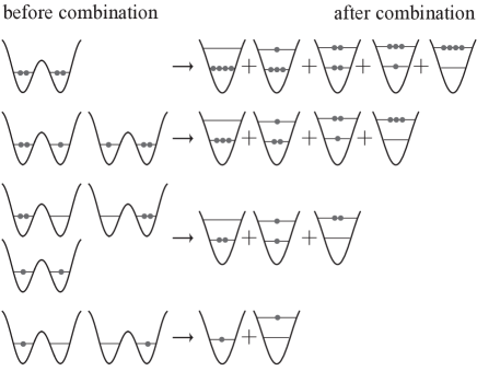
Figure 4: Analysis of the process of combining the two initial replicas, showing possible states with at most double occupation (dots) in a given well before combination of the layers (left hand side), and the resulting possible states after combination of the layers (right hand side). Note that here ‘$+$’ indicates a general superposition with unspecified coefficients, as these are dependent on the precise time dependence of system dynamics during combination. Knowledge of these coefficients is not necessary in the measurement scheme presented here.

In the next section we show how the different configurations for a given particle number can be measured and thus the total occupation numbers determined.

III.2.3 Number Distribution Characterization

We now investigate a scheme similar to the one presented in Campbell et al. (2006) that uses density-dependent energy shifts to spectroscopically distinguish different particle numbers at each site of the combined layer (see section III.2.2 above) resulting in a measurement of $p_{n}$. The measurement of $p_{n}^{\alpha,\beta}$ follows from the same spectroscopic analysis, but performed on each individual layer $\alpha$, $\beta$ before combining the layers. Such a scheme has already been implemented experimentally and was utilized to observed the Mott-insulating shell structure that arises due to a harmonic trapping potential commonly present in cold atomic gases experiments Campbell et al. (2006).

We begin with all atoms in an internal state $a$, and investigate the weak coupling of particles to a second internal state $b$ (with at most one particle transferred). Due to the difference in interaction energy between particles of species $a$ and $b$, and particles solely of species $a$ there is an energy shift between the “initial” state (all particles of species $a$) and “final” state (one particle of species $b$ and all others particles of species $a$). Thus different initial particle numbers can be distinguished by the energy shift (corresponding to the Raman detuning at which the transfer is resonant), provided the shift is different for the different particle numbers. Since particles in the combined layer can be spread across multiple motional states (see section III.2.2 above), different energy shifts occur for different configurations of the same number of particles. Whilst we find that the energy shifts of some of the configurations (of the same number of particles) are identical or very similar, there are other configurations having substantially different energy shifts. Thus we have to check that the energy shifts for all configurations of a given number of particles can be distinguished from energy shifts of configurations corresponding to a different total number of particles. To this end we now present a detailed calculation of the energy shifts arising from all the different initial configurations of particles and show in which cases the total number of particles can be distinguished.

Let $a_{k}^{\dagger}$ and $b_{k}^{\dagger}$ denote the creation operators for particles of species $a$ and $b$, respectively, in band $k$ where $k\in\{0,1\}$. Then the Raman coupling between the two internal states $a$ and $b$ is described by an effective Hamiltonian (within a rotating-wave approximation)

$$H_{\rm\scriptscriptstyle RC}=\frac{\Omega(t)}{2}(a^{\dagger}_{0}b_{0}+a^{\dagger}_{1}b_{1}+\textrm{H.c.})-\Delta(t)(b_{0}^{\dagger}b_{0}+b_{1}^{\dagger}b_{1}),$$ (15)

where $\Delta(t)$ is the Raman detuning, $\Omega(t)$ the effective two-photon Rabi frequency, and we have assumed that $\Omega(t)\ll\Delta^{\prime}$ where $\Delta^{\prime}$ are the detunings of the lasers from the atomic excited state. In what follows we assume that $\int\Omega(t)dt\ll\pi$, i.e., weak coupling to internal state $b$ and that the two lasers creating the Raman transition are running waves with equal wave vectors. Note that processes in which the internal state and the band would change do not occur provided the Raman detuning and effective two-photon Rabi frequency are smaller than the band separation.

The onsite interaction energy for atoms of species $a$ and $b$ in the lowest two bands is described by the following Hamiltonian

$$H_{\rm\scriptscriptstyle int} = \sum_{i\in\{a,b\}}\bigg{[}\frac{U_{00}^{ii}}{2}n_{0}^{i}(n_{0}^{i}-1)+\frac{U_{11}^{ii}}{2}n_{1}^{i}(n_{1}^{i}-1)$$

$$+2U_{01}^{ii}n_{0}^{i}n_{1}^{i}\bigg{]}+U_{00}^{ab}n_{0}^{a}n_{0}^{b}+U_{11}^{ab}n_{1}^{a}n_{1}^{b}+U_{01}^{ab}\left[n_{0}^{a}n_{1}^{b}\right.$$

$$\left.+n_{1}^{a}n_{0}^{b}+(a_{0}^{\dagger}a_{1}b_{1}^{\dagger}b_{0}+a_{1}^{\dagger}a_{0}b_{0}^{\dagger}b_{1}+\textrm{H.c.})\right],$$

where

$$U_{kl}^{ij}=2\omega_{\perp}a_{ij}\int dz|w_{k}(z)|^{2}|w_{l}(z)|^{2},$$ (17)

with $a_{ij}$ the scattering length between two particles in internal states $i$ and $j$ ($i,j\in\{a,b\}$), $\omega_{\perp}$ the transverse trapping frequency, and $w_{k}(z)$ the Wannier functions corresponding to band $k$ ($k,l\in\{0,1\}$). Note we have also introduced the particle number operators $n_{k}^{a}=a_{k}^{\dagger}a_{k}$ and $n_{k}^{b}=b_{k}^{\dagger}b_{k}$. We further make the assumption that the lattice is very deep so that we can approximate all the Wannier functions by simple harmonic oscillator eigenfunctions. This assumption of a deep lattice gives the following simplified expressions $2U_{01}^{ij}=U_{00}^{ij}$ and $U_{11}^{ij}=(3/4)U_{00}^{ij}$.

Using (LABEL:hamiltonian_two_bands_two_species) we now explicitly compute the energy shift $\Delta E=E_{f}-E_{i}$ associated with the processes $|i\rangle\rightarrow|f\rangle$, where $|i\rangle$ is the initial state corresponding to all particles of species $a$ and having energy $E_{i}$, and $|f\rangle$ is the final state corresponding to one particle transferred to internal state $b$ and having energy $E_{f}$. Clearly, $\Delta E$ depends on how the particles are initially distributed in the lower and higher bands after combining the two layers (see the right hand side of figure 4). There are two different cases to be considered; either all particles are initially in the same band (this is the situation in Campbell et al. (2006)) or particles are initially in both bands. In the latter case it is then possible that particles in either band are transferred to internal state $b$ and since these different possible resulting states are coupled by the interaction Hamiltonian in (LABEL:hamiltonian_two_bands_two_species) the final resulting state is a superposition of these, corresponding to an eigenstate of the Hamiltonian in (LABEL:hamiltonian_two_bands_two_species).

For example, let us consider a total initial number of two particles as depicted in figure 5. The different initial and final states are most conveniently expressed in the occupation number basis $|N_{0}^{a},N_{1}^{a};N_{0}^{b},N_{1}^{b}\rangle$ with $N_{0}^{a,b}$ ($N_{1}^{a,b}$) the number of particles of species $a$, $b$ in the lower (higher) band at a given lattice site. First consider the case where both particles are initially in the lower or higher bands corresponding to the initial states $|2,0;0,0\rangle$ or $|0,2;0,0\rangle$ (see top and bottom of figure 5). The corresponding final states are given by $|1,0;1,0\rangle$ and $|0,1;0,1\rangle$, and the corresponding energy shifts are $\Delta E/U_{00}^{aa}=\epsilon-1$ and $\Delta E/U_{00}^{aa}=\frac{3}{4}(\epsilon-1)$, where we have defined $\epsilon\equiv U_{00}^{ab}/U_{00}^{aa}$. Next we consider the case where there is a particle in each band initially corresponding to the initial state $|1,1;0,0\rangle$ (see middle of figure 5). Then the corresponding final states are the eigenstates of the Hamiltonian in (LABEL:hamiltonian_two_bands_two_species) in the subspace corresponding to one particle of species $a$ and one particle of species $b$ given by $|1,1\rangle_{\pm}\equiv(1/\sqrt{2})\left(|0,1;1,0\rangle\pm|1,0;0,1\rangle\right)$, with eigenenergies $E_{+}/U_{00}^{aa}=\epsilon$ and $E_{-}/U_{00}^{aa}=0$. The associated energy shifts for these two possible final states are $\Delta E/U_{00}^{aa}=\epsilon-1$ and $\Delta E/U_{00}^{aa}=-1$ respectively. Note that the Raman transition only couples the state $|1,1\rangle_{+}$ to the initial state $|1,1;0,0\rangle$ with a matrix coupling element $\Omega_{fi}=\sqrt{2}$, where $\Omega_{fi}\equiv\langle f|H_{\rm\scriptscriptstyle RC}|i\rangle$, while for the state $|1,1\rangle_{-}$ we find $\Omega_{fi}=0$. Figure 5 summarizes the different possible configurations for a total of two particles together with the corresponding energy shift $\Delta E$ and matrix coupling element $\Omega_{fi}$. We note that the energy shifts, $\Delta E$, for the different final states to which the initial states couple (i.e., $\Omega_{fi}\neq 0$) are very similar, this is of advantage since our scheme needs only to distinguish energy shifts for different total particle numbers.

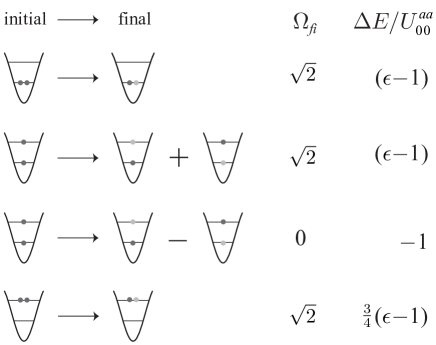
Figure 5: Illustration of the number distribution characterization within the two layers for states with two particles in the combined layer. On the left are all possible initial configurations of two particles of species $a$ in the combined lattice (dark-coloured circles) and the corresponding final states with one particle each of species $a$ and $b$ (light-coloured circles). On the right we list the respective coupling matrix elements, $\Omega_{fi}$, and energy shifts, $\Delta E/U_{00}^{aa}$, for each of the configurations on the left.

Similarly, we can determine the energy shifts and coupling matrix elements for other numbers of particles. If all particles are initially in the lower or higher state corresponding to the initial states $|N_{0}^{a},0;0,0\rangle$ or $|0,N_{1}^{a};0,0\rangle$, the corresponding final states are given by $|N_{0}^{a}-1,0;1,0\rangle$ and $|0,N_{1}^{a}-1;0,1\rangle$. The corresponding energy shifts are then given by $\Delta E/U_{00}^{aa}=(N_{0}^{a}-1)(\epsilon-1)$ and $\Delta E/U_{00}^{aa}=\frac{3}{4}(N_{1}^{a}-1)(\epsilon-1)$, and the matrix coupling element in each case is $\Omega_{fi}=\sqrt{N_{0}^{a}}$ and $\Omega_{fi}=\sqrt{N_{1}^{a}}$ respectively. For other initial configurations with $m$ particles in the lower band and $n$ particles in the higher band the corresponding final states are found by diagonalizing the Hamiltonian in  (LABEL:hamiltonian_two_bands_two_species) in the appropriate particle subspace. This always results in a pair of eigenstates denoted $|m,n\rangle_{\pm}$ with eigenenergy $E_{\pm}^{(m,n)}$ and using these expressions the energy shift $\Delta E$ and coupling matrix elements $\Omega_{fi}$ can be directly determined. For a total initial number of three and four particles the expressions for $|m,n\rangle_{\pm}$, $E_{\pm}^{(m,n)}$, $\Delta E$ and $\Omega_{fi}$ are given in appendix  A.1 and A.2, respectively, for all the different initial configurations. In table 1 we list the results for up to a maximum number of four particles; the first column lists the different initial configurations and corresponding final states, the second column lists the corresponding matrix coupling elements $\Omega_{fi}$ and the third column lists the associated energy shifts $\Delta E$.

It is possible to distinguish different occupation numbers for specific ranges of $\epsilon$ if the energy shifts for different total numbers of particles are distinct. The desired range of $\epsilon$ is then between points where any energy shifts for different total number of particles would coincide (e.g., $\epsilon=1$) com (e). For a specific example we consider the value $\epsilon=0.98$ (corresponding to scattering length values in Campbell et al. (2006)) and give numerical values for the matrix coupling elements $\Omega_{fi}$ and the energy shifts $\Delta E$ in columns four and five, respectively, in table 1. Then, to a high accuracy, the determination of $p_{n}$ is obtained by applying the coupling between the different internal states $a$ and $b$ for a short time $t_{n}=\Delta t/\sqrt{n}$ at all resonant frequencies in table 1 with total number of particles $n$ (ignoring the resonances with small and vanishing couplings $\Omega_{fi}$). The total number of transferred particles is then proportional to $p_{n}$ and efficiently avoids problems arising from non-adiabatic combination of the layers.

Table 1: Resonant energies and coupling strengths for the transfer of single atoms in the combined layer to a different internal state. Column one lists the different initial configurations and the corresponding final states up to a maximum number of four particles. In the second and third column we list the matrix coupling elements $\Omega_{fi}$ and energy shifts $\Delta E$, respectively, corresponding to the different initial configurations in the first column. The states $|m,n\rangle_{\pm}$ are listed in the text and appendices together with the corresponding eigenenergies $E_{\pm}^{(m,n)}$ and coupling matrix elements $\eta_{\pm}^{(m,n)}$. The last two columns give numerical values of $\Omega_{fi}$ and $\Delta E$ for the specific value $\epsilon=0.98$.

$|i\rangle\rightarrow|f\rangle$	$\Omega_{fi}$	$\Delta E/U_{00}^{aa}$	$\Omega_{fi}$	$\Delta E/U_{00}^{aa}$
$|1,0;0,0\rangle\rightarrow|0,0;1,0\rangle$	1	0	1	0
$|0,1;0,0\rangle\rightarrow|0,0;0,1\rangle$	1	0	1	0
$|2,0;0,0\rangle\rightarrow|1,0;1,0\rangle$	$\sqrt{2}$	$\frac{3}{4}(\epsilon-1)$	1.4	-.018
$|2,0;0,0\rangle\rightarrow|1,0;1,0\rangle$	$\sqrt{2}$	$(\epsilon-1)$	1.4	-.024
$|1,1;0,0\rangle\rightarrow|1,1\rangle_{+}$	$\sqrt{2}$	$(\epsilon-1)$	1.4	-.024
$|1,1;0,0\rangle\rightarrow|1,1\rangle_{-}$	0	-1	0	-1
$|3,0;0,0\rangle\rightarrow|2,0;1,0\rangle$	$\sqrt{3}$	$2(\epsilon-1)$	1.7	-.049
$|2,1;0,0\rangle\rightarrow|2,1\rangle_{+}$	$\sqrt{3}$	$2(\epsilon-1)$	1.7	-.049
$|2,1;0,0\rangle\rightarrow|2,1\rangle_{-}$	0	$\frac{\epsilon}{2}-2$	0	-1.5
$|1,2;0,0\rangle\rightarrow|1,2\rangle_{+}$	$\eta_{+}^{(1,2)}$	$E_{+}^{(1,2)}-3$	1.7	-.29
$|1,2;0,0\rangle\rightarrow|1,2\rangle_{-}$	$\eta_{-}^{(1,2)}$	$E_{-}^{(1,2)}-3$	-.0034	-1.8
$|0,3;0,0\rangle\rightarrow|0,2;0,1\rangle$	$\sqrt{3}$	$\frac{3}{2}(\epsilon-1)$	1.7	-.037
$|4,0;0,0\rangle\rightarrow|3,0;1,0\rangle$	$\sqrt{4}$	$3(\epsilon-1)$	2	-.073
$|3,1;0,0\rangle\rightarrow|3,1\rangle_{+}$	$\sqrt{4}$	$3(\epsilon-1)$	2	-.073
$|3,1;0,0\rangle\rightarrow|3,1\rangle_{-}$	0	$\epsilon-3$	0	-2.0
$|2,2;0,0\rangle\rightarrow|2,2\rangle_{+}$	$\eta_{+}^{(2,2)}$	$E_{+}^{(2,2)}-\frac{23}{4}$	2.0	-0.070
$|2,2;0,0\rangle\rightarrow|2,2\rangle_{-}$	$\eta_{-}^{(2,2)}$	$E_{-}^{(2,2)}-\frac{23}{4}$	-.0031	-2.0
$|1,3;0,0\rangle\rightarrow|1,3\rangle_{+}$	$\eta_{+}^{(1,3)}$	$E_{+}^{(1,3)}-\frac{15}{4}$	2.0	1.4
$|1,3;0,0\rangle\rightarrow|1,3\rangle_{-}$	$\eta_{-}^{(1,3)}$	$E_{-}^{(1,3)}-\frac{15}{4}$	-.0054	-.52
$|0,4;0,0\rangle\rightarrow|0,3;0,1\rangle$	$\sqrt{4}$	$\frac{9}{4}(\epsilon-1)$	2	-.055

IV Overlap Function in the Disordered Bose-Hubbard model

In this section we determine the overlap function $q$ [see (4)] in the disorder Bose-Hubbard model, both analytically and numerically. We focus on a bimodal disorder potential $\Delta_{i}=\pm\Delta$ with the probability distribution $P(\Delta)=1-P(-\Delta)=p$, which is the appropriate description for the chosen disorder implementation (see discussion in earlier sections). In the following, we present the modifications due to the presence of a weak ($\Delta<U/2$) bimodal disorder potential, and the prediction for the overlap function within the different phases (see figure 2). It follows from this constraint that we do not enter the compressible disordered phase, and hence the system will always have a unique ground state. Thus, the ground states in two exact copies $\alpha$, $\beta$ of the system (i.e. same disorder distribution) are the same, and consequently $\langle n_{i}^{\alpha}\rangle=\langle n_{i}^{\beta}\rangle$. We therefore expect a Sherrington-Kirkpatrick-type behaviour for the overlap Sherrington and Kirkpatrick (1975), i.e. the overlap between any two copies will always be the same, and thus the overlap function $q$ can in fact be calculated using (3).

While the above is a self-evident statement for a replica-symmetric system such as the one we examine here, it may no longer be true for systems thought to exhibit replica-symmetry breaking (e.g. a classical spin glass type model Parisi (1983), or quantum systems with extended interactions Giamarchi et al. (2001)). For the latter type of system, measurement of the overlap function using physical replicas (see section III) is thought to yield different values for the overlap depending on $\alpha$ and $\beta$, the defining signature of replica symmetry-breaking.

In section IV.1 we analytically calculate the overlap function, for the various phases of the disorder Bose-Hubbard model (1), whilst in section  IV.2 we present results for the overlap function from numerical simulation of the one-dimensional system.

IV.1 Analytical determination of the overlap function

Starting with the limit of vanishing hopping $J=0$, (1) reduces to an onsite Hamiltonian and the ground state is given by $|\Omega\rangle=\Pi_{i}|\Omega\rangle_{i}$ with $|\Omega\rangle_{i}$ the lowest energy state within each site $i$. This lowest energy states takes the form $|\Omega\rangle_{i}=|n_{i}\rangle$ with $|n_{i}\rangle$ being a state with fixed particle number $n_{i}$ at site $i$, with $n_{i}$ subject to the constraint

$$U\left(n_{i}-1\right)<\mu-\Delta_{i}<Un_{i}.$$ (18)

For a weak bimodal disorder potential ($\Delta<U/2$), we have to distinguish two different cases.

First, for a chemical potential within the range $U(n_{0}-1)+\Delta<\mu<Un_{0}-\Delta$ the above constraint in (18) is fulfilled independently of the site parameter $i$ for the integer value $n_{0}$, i.e., at each site the ground state is characterized by the integer particle density $[\langle n_{i}\rangle]_{av}=n_{0}$ and we obtain a Mott-insulator (MI) phase (see figure 2). Furthermore, the overlap parameter vanishes identically in this limit, i.e., $q=0$ for a Mott-insulator at $J=0$.

Second, for chemical potentials in the range $Un_{0}-\Delta<\mu<Un_{0}+\Delta$, the particle number at sites with different disorder potential $\Delta_{i}$ differs by a single particle, i.e., at each site with disorder potential $\Delta_{i}=\Delta$ the particle number is determined by $n_{0}$, while at sites with disorder potential $\Delta_{i}=-\Delta$ the lowest energy state is characterized by $n_{0}+1$ particles. Therefore, the averaged particle density and the overlap parameter take the form

$$[\langle n_{i}\rangle]_{av}=n_{0}+(1-p)\hskip 28.45274ptq=p(1-p).$$ (19)

This situation corresponds to the disorder-induced Bose-glass (BG) phase (see figure 2) and the ground state is characterized by nonhomogeneous filling. Similarly to the case of the MI phase, the particle number is fixed over a finite range of the chemical potential and thus the BG is incompressible. In contrast to the MI phase, the BG phase is characterized by a non-vanishing overlap parameter dependent on $p$.

Next, we focus on small hopping, $J\ll U,\Delta,\mu$, and determine the overlap function using perturbation theory. We seek a unitary transformation of the form $U=e^{-iS}$ which transforms the total Hamiltonian in (1) to an effective Hamiltonian having the same eigenspectrum but acting only in the space of the unperturbed eigenstates. Using this unitary transformation we can directly determine the corrections due to hopping in perturbation theory by computing $\langle\Omega|\tilde{n}_{i}|\Omega\rangle$ where $\tilde{n}_{i}\equiv U^{\dagger}n_{i}U$. Details are given in appendix  B.

We start with the Mott-insulator and consider the leading order (non-vanishing) correction to the overlap function which occurs at fourth order due to a site (disorder) independent density, $\langle\Omega|n_{i}|\Omega\rangle=n_{0}$ (using $|\Omega\rangle_{i}=|n_{0}\rangle$ in the MI). To lowest order in perturbation theory the overlap is then given by

$$q=J^{4}\left([\langle\tilde{A}_{2}\rangle^{2}]_{av}-[\langle\tilde{A}_{2}\rangle]_{av}^{2}\right),$$ (20)

where

$$\tilde{A}_{2}=-\frac{1}{2}[S_{1},[S_{1},n_{i}]],$$ (21)

with

$$S_{1}=-i\sum_{\langle jk\rangle}c_{jk}|\Omega\rangle\langle\phi_{jk}|+\textrm{H.c.}$$ (22)

and $|\phi_{jk}\rangle=|n_{0}+1\rangle_{j}|n_{0}-1\rangle_{k}\Pi_{l\neq ij}|n_{0}\rangle_{l}$. Using these expressions it is straightforward to compute the expectation value of the density correction

$$\langle\tilde{A}_{2}\rangle=n_{0}(n_{0}+1)\sum_{\langle j(i)\rangle}\left(\frac{1}{(E_{0}-E_{ij})^{2}}-\frac{1}{(E_{0}-E_{ji})^{2}}\right),$$ (23)

where $E_{0}-E_{ij}=-U+\Delta_{j}-\Delta_{i}$. It is now straightforward to calculate the disorder averages and the overlap is given by

$$q=64(n_{0}(n_{0}+1))^{2}p(1-p)z(z+1)\frac{J^{4}U^{2}\Delta^{2}}{(U^{2}-4\Delta^{2})^{4}},$$ (24)

where $z$ is the number of nearest neighbours.

Next we turn to the Bose-glass phase and consider the leading order (non-vanishing) correction to the overlap function which occurs here at second order. The expression for the overlap in lowest-order perturbation theory is then given by

$$q=q_{0}+J^{2}\left([\langle n_{i}\rangle\langle\tilde{A}_{2}\rangle]_{av}-[\langle n_{i}\rangle]_{av}[\langle\tilde{A}_{2}\rangle]_{av}\right),$$ (25)

where $q_{0}=p(1-p)$ (the overlap at zero hopping), $\tilde{A}_{2}$ and $S_{1}$ are as given above for the MI phase but with

$$|\Omega\rangle=\prod_{l}\left[d_{l}|n_{0}+1\rangle_{l}+(1-d_{l})|n_{0}\rangle_{l}\right]$$ (26)

and

$$\begin{split}|\phi_{jk}\rangle=\left[d_{j}|n_{0}+2\rangle_{j}+(1-d_{j})|n_{0}+1\rangle_{j}\right][d_{k}|n_{0}\rangle_{k}\\ +(1-d_{k})|n_{0}-1\rangle_{k}]\Pi_{l\neq jk}[d_{l}|n_{0}+1\rangle_{l}+(1-d_{l})|n_{0}\rangle_{l}],\end{split}$$

where $d_{j,k,l}$ $(1-d_{j,k,l})$ is zero (one) for $\Delta_{j,k,l}=\Delta$ ($\Delta_{j,k,l}=-\Delta$). Again, using these expressions it is straightforward to compute the expectation value of the density correction and for $n_{0}\geq 1$ we obtain

$$\langle\tilde{A}_{2}\rangle=\sum_{\langle j(i)\rangle}\left(\frac{\gamma_{ij}^{2}}{(E_{0}-E_{ij})^{2}}-\frac{\gamma_{ji}^{2}}{(E_{0}-E_{ji})^{2}}\right),$$ (27)

where

$$E_{0}-E_{ij}=-U(1-d_{i}+d_{j})+\Delta_{j}-\Delta_{i}$$ (28)

and

$$\gamma_{ij} = (d_{i}\sqrt{n_{0}+2}$$

$$+(1-d_{i})\sqrt{n_{0}+1})(d_{j}\sqrt{n_{0}+1}+(1-d_{j})\sqrt{n_{0}}).$$

Once again a straightforward calculation of the disorder averages gives the following expression ($n_{0}\geq 1$) for the overlap:

$$q=p(1-p)\left(1-J^{2}\frac{(n_{0}+1)^{2}U(U-2\Delta)+\Delta^{2}}{2\Delta^{2}(U-\Delta)^{2}}\right).$$ (30)

An analogous calculation for $n_{0}=0$ gives

$$q=p(1-p)\left(1-\frac{J^{2}}{2\Delta^{2}}\right)$$ (31)

which corresponds to the $U\rightarrow 0$ limit of (30).

When the effects of hopping dominate, the bosonic atoms are in the superfluid phase (see figure 2). Then, the influence of weak disorder on the superfluid phase can be studied within a generalized mean-field approach. In analogy to the Gross-Pitaevskii formalism, we replace the bosonic operators $b_{i}$ in the Hamiltonian (1) by a local complex field $\psi_{i}$, and minimize the corresponding free energy functional $H(\psi_{i})$. The effect of disorder is to produce fluctuations in the local density. Hence we make the ansatz $\psi_{i}=e^{i\phi}\sqrt{n_{0}+\delta n_{i}}$ where $n_{0}$ is the homogeneous density in the absence of disorder and $\delta n_{i}\propto\Delta_{i}$ is the disorder induced density fluctuation. Introducing the notation $\delta n=[\delta n_{i}]_{av}$ as the disorder-averaged density fluctuation, the particle density reduces to $[\langle n_{i}\rangle]_{av}=n_{0}+\delta n$. We substitute this ansatz into $H(\psi_{i})$, expand $\psi_{i}$ for small fluctuations, $\delta n_{i}\ll n_{0}$ (see appendix C) and minimize the resulting expression in (74) at fixed particle number, which is equivalent to requiring $[\delta n_{i}]_{av}=0$. Note that for large dimension and thus a large number of nearest neighbours we may replace

$$\sum_{\langle j(i)\rangle}\delta n_{j}\approx z\delta n.$$ (32)

Using this relation and self-consistently solving for the density fluctuations $\delta n_{i}$ (see appendix C) gives the overlap function

$$q=\left(\frac{4n_{0}\Delta}{2Un_{0}+zJ}\right)^{2}p(1-p),$$ (33)

where $n_{0}=(\mu+Jz)/U+\frac{1}{2}$.

In summary, we find that in the limit of small hopping $J/U\ll 1$, the overlap signals a sharp crossover between the Mott-insulator with $q\approx 0$ and the Bose-glass with $q\approx p(1-q)$, see figure 2. In turn, the superfluid phase is characterized by off-diagonal long range order giving rise to coherence peaks in a time of flight picture. Consequently, the overlap and the coherence peaks in time of flight allow for a clear identification of the phases in the disordered Bose-Hubbard model. However, we would like to point out that the overlap function behaves smoothly across the phase transition and consequently is not suitable for the precise determination of the exact location of the phase transition.

IV.2 Numerical results

We have simulated the disordered Bose-Hubbard model (1) in 1D using a number-conserving algorithm based on time-dependent matrix product states Vidal (2003, 2004). In the matrix product state representations, we reduce the Hilbert space by retaining only the $\chi$ most significant components in a Schmidt-decomposition of the state at each possible bipartite splitting of the system. States in 1D can be efficiently represented in this way, with relatively small $\chi$ giving essentially unity overlap between the represented state and the actual state. The simulations both serve as a check for the perturbation theory, and allow computation of the overlap function beyond the perturbation limit from the microscopic model.

Because we consider the regime $2\Delta<U$, the system remains incompressible and does not enter the disordered glass phase. Therefore we do not expect replica-symmetry breaking to occur. For our simulations, the presence of replica-symmetry is equivalent to convergence to a unique ground-state for any given disorder independent of initial conditions. The overlap function can then be computed as

$$q=\frac{1}{L}\sum_{i}\langle n_{i}\rangle^{2}-\overline{n}^{2}$$ (34)

where $\overline{n}$ is the density of the system. Computation of the overlap function can be simplified in this way as $L^{-1}\sum_{i}\langle n_{i}\rangle$ self-averages to $[\langle n_{i}\rangle]_{av}$ for sufficiently large systems, which in turn self-averages to $\overline{n}$.

The ground states used in (34) are computed by imaginary-time evolution, c.f. Vidal (2004), of the 1D Bose-Hubbard-model given by (1) with a randomly-chosen bimodal distribution, and different impurity strengths $2\Delta$. The lattice size is $L=64$, representative of current experimental capabilities, and we compute the overlap as a function of $\Delta$ for several different values of $U/J$ and the fraction of impurity-occupied sites, $p$. In figure 6 we display results for $U/J=10$ and $p=0.5$. We have performed convergence tests in the time step, the duration of imaginary-time evolution, the number of disorder realizations, and the number of retained states $\chi$. We find that the overlap function converged even for surprisingly small values of $\chi\sim 20$ states in the large $U/J$ limit (Mott-insulator or Bose-glass regime). Regarding the number of disorder realizations for each value of $\Delta$, we find that whilst $10$ random realizations of bimodal disorder are not sufficient to narrow the error down, $20$ realizations suffice. Much of the observed fluctuations in the value of the overlap function for a given $\Delta$ stem from the fact that we allow the number of impurities in each realization to fluctuate around the mean $Lp$. Conversely, in our simulation data we observe different disorder realizations with the same number of impurities having overlaps closer to each other than the error bars is figure 6 would suggest.

As shown in figure 6, we generally found very good agreement between numerical simulations and perturbation theory in its region of validity. For the Mott-insulator regime (commensurate filling factor) this is the regime where $2\Delta\ll U$. We observe the breakdown of our second-order perturbation theory as $\Delta$ approaches $U/2=5J$, which is caused by energy-degeneracy of adjacent impurity- and non-impurity occupied sites when $\Delta=U/2$. In the Bose-glass regime, breakdown of perturbation theory sets in for low $\Delta$, as degeneracy occurs there for $\Delta=0$.

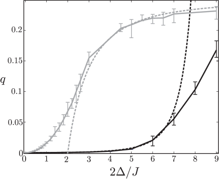
Figure 6: Overlap function $q$ as a function of impurity strength $\Delta$ in the Mott-insulating phase at filling factor $n_{0}=1$ (black lines) and in the Bose-glass phase for $n_{0}=0$ (grey lines). In both cases, the impurity probability is $p=0.5$ and $U/J=10$, for $L=64$. Simulation results (solid lines) are shown versus results from perturbation theory (dashed lines). Much of the variation in the simulated overlap function is due to the fact that we allow the number of impurities to fluctuate around the value given by $Lp$ in each particular disorder realization. Note that the perturbation result in the Mott-insulator diverges as $\Delta$ approaches $U$ due to energy degeneracy [c.f.  (24)]. In the Bose-glass phase, second-order perturbation theory yields a divergence as $\Delta$ approaches $0$, again due to energy degeneracy [c.f. (31)].

V Conclusion

We have shown how the Bose-glass phase can be identified by measuring the overlap function characterizing the correlations between disorder replicas, i.e., systems having identical disorder landscape. We have described a procedure to create disorder replicas using cold atomic gases in an optical lattice, focusing on the case of disorder induced by a second atomic species. A scheme to measure the overlap has been presented, which involves the characterization of the occupation numbers in both the individual replicas and the joint system, where both replicas have been combined. Specifically, we have shown that after combining the replicas together, particles can be distributed across multiple motional states and we explained in detail how to determine the occupation number distribution in this situation. Using perturbation theory we have calculated the overlap for weak hopping and have shown the different behaviours exhibited in the Mott-insulator and Bose glass phases; these results are in good agreement with the results from a one-dimensional numerical simulation. In the opposite limit of very large hopping we also obtain analytical results for the overlap within a mean-field-theory treatment.

Applying our proposed measurement scheme for the overlap to other types of disordered models Giamarchi et al. (2001); Parisi (1983) would provide interesting insights to characteristic properties of disorder-induced quantum phases, such as the possible appearance of broken ergodicity and different degenerate ground states. Of particular interest would be the quantum spin glass where the overlap corresponds to the Edwards-Anderson order parameter which has been conjectured to exhibit replica symmetry breaking Parisi (1983), i.e., the results for the overlap depend on the particular replica. Our method could also give novel insights into physics of systems that possess multiple metastable states, such as ultracold dipolar gases Menotti et al. (2007) or quantum emulsions Roscilde and Cirac (2007); in particular statistics of overlaps of such metastable states could be measured. In addition to equilibrium properties considered here, the dynamics of the overlap might also posses an interesting behaviour, and could be measured in a similar setup. In one-dimension the time evolution of the overlap could be determined numerically Vidal (2004).

Appendix A Energy shifts and couplings for three and four particles

In the following two sections we determine expressions for the eigenstates and eigenenergies of  (LABEL:hamiltonian_two_bands_two_species), i.e., $|m,n\rangle_{\pm}$ and $E_{\pm}^{(mn)}$ and associated energy shifts and couplings for all possible initial configurations of three and four particles. Note that the case where all particles are in the lowest or highest energy band has already been explained in section III.2.3 and will not be discussed here further.

A.1 Three Particles

We consider the two different configurations described by the initial states i) $|2,1;0,0\rangle$ and ii) $|1,2;0,0\rangle$.

For case i) the two eigenstates are given by

$$|2,1\rangle_{+} = \frac{1}{\sqrt{3}}(|2,0;0,1\rangle+\sqrt{2}|1,1;1,0\rangle),$$ (35)

$$|2,1\rangle_{-} = \frac{1}{\sqrt{3}}(-\sqrt{2}|2,0;0,1\rangle+|1,1;1,0\rangle)$$ (36)

with eigenenergies $E_{+}^{(2,1)}=2\epsilon+1$ and $E_{-}^{(2,1)}=\epsilon/2+1$ respectively. We see that only the state $|2,1\rangle_{+}$ couples to the initial state $|2,1;0,0\rangle$, with a matrix coupling element of $\Omega_{fi}=\sqrt{3}$, whilst for the state $|2,1\rangle_{-}$ we find $\Omega_{fi}=0$. The energy shifts for the two different possible processes are given by $\Delta E/U_{00}^{aa}=2(\epsilon-1)$ and $\Delta E/U_{00}^{aa}=\frac{\epsilon}{2}-2$.

For case ii) the two eigenstates are given by

$$|1,2\rangle_{\pm} = \frac{1}{\sqrt{1+(\gamma_{\pm}^{(1,2)})^{2}}}\left(\gamma_{\pm}^{(1,2)}|0,2;1,0\rangle+|1,1;0,1\rangle\right),$$

where

$$\gamma_{\pm}^{(1,2)} = \frac{-1-\epsilon\pm\sqrt{33\epsilon^{2}+2\epsilon+1}}{4\sqrt{2}\epsilon},$$ (38)

and with eigenenergies

$$E_{\pm}^{(1,2)} = \epsilon+1\pm\frac{1}{8}\sqrt{33\epsilon^{2}+2\epsilon+1}+\frac{1}{8}(\epsilon-1).$$

In this case both states $|1,2\rangle_{\pm}$ have nonzero coupling to the state $|1,2;0,0\rangle$ given by

$$\Omega_{fi} = \eta_{\pm}^{(1,2)}\equiv\langle 1,2|_{\pm}H_{\rm\scriptscriptstyle RC}|1,2;0,0\rangle$$

$$= \frac{1}{\sqrt{1+(\gamma_{\pm}^{(1,2)})^{2}}}(\gamma_{\pm}^{(1,2)}+\sqrt{2}).$$

The energy shifts for the two different possible processes are given by $\Delta E/U_{00}^{aa}=E_{\pm}^{(1,2)}-3$.

A.2 Four Particles

We consider the three different configurations described by the initial states i) $|3,1;0,0\rangle$, ii) $|2,2;0,0\rangle$ and iii) $|1,3;0,0\rangle$.

For case i) the eigenstates are given by

$$|3,1\rangle_{+} = \frac{1}{\sqrt{4}}(|3,0;0,1\rangle+\sqrt{3}|2,1;1,0\rangle),$$ (41)

$$|3,1\rangle_{-} = \frac{1}{\sqrt{4}}(-\sqrt{3}|3,0;0,1\rangle+|2,1;1,0\rangle),$$ (42)

with eigenenergies $E_{+}^{(3,1)}=3(\epsilon+1)$ and $E_{-}^{(3,1)}=\epsilon+3$, respectively. We see that only the state $|3,1\rangle_{+}$ couples to the initial state $|3,1;0,0\rangle$, with a matrix coupling element of $\Omega_{fi}=\sqrt{4}$, whilst for the state $|3,1\rangle_{-}$ we find $\Omega_{fi}=0$. The energy shifts for the two different possible processes are given by $\Delta E/U_{00}^{aa}=3(\epsilon-1)$ and $\Delta E/U_{00}^{aa}=\epsilon-3$.

For case ii) the eigenstates are given by

$$|2,2\rangle_{\pm} = \frac{1}{\sqrt{1+(\gamma_{\pm}^{(2,2)})^{2}}}\left(\gamma_{\pm}^{2,2}|1,2;1,0\rangle+|2,1;0,1\rangle\right),$$

where

$$\gamma_{\pm}^{(2,2)} = \frac{-1+\epsilon\pm\sqrt{65\epsilon^{2}-2\epsilon+1}}{8\epsilon},$$ (44)

and with eigenenergies

$$E_{\pm}^{(2,2)} = 3+2\epsilon\pm\sqrt{65\epsilon^{2}-2\epsilon+1}-\frac{1}{8}(1+\epsilon).$$

In this case, generally both states $|2,2\rangle_{\pm}$ have nonzero coupling to the state $|2,2;0,0\rangle$ given by

$$\Omega_{fi} = \eta_{\pm}^{(2,2)}\equiv\langle 2,2|_{\pm}H_{\rm\scriptscriptstyle RC}|2,2;0,0\rangle$$

$$= \sqrt{\frac{2}{1+(\gamma_{\pm}^{(2,2)})^{2}}}(\gamma_{\pm}^{(2,2)}+1).$$

The energy shifts for the two different possible processes are given by $\Delta E/U_{00}^{aa}=E_{\pm}^{(2,2)}-\frac{23}{4}$.

For case iii) the eigenstates are given by

$$|1,3\rangle_{\pm} = \frac{1}{\sqrt{1+(\gamma_{\pm}^{(1,3)})^{2}}}\left(\gamma_{\pm}^{(1,3)}|0,3;1,0\rangle+|1,2;0,1\rangle\right),$$

where

$$\gamma_{\pm}^{(1,3)} = \frac{-1-\epsilon\pm\sqrt{13\epsilon^{2}+2\epsilon+1}}{2\sqrt{3}\epsilon},$$ (48)

and with eigenenergies

$$E_{\pm}^{(1,3)} = 3+2\epsilon\pm\sqrt{13\epsilon^{2}+2\epsilon+1}-\frac{1}{4}(2+\epsilon).$$

In this case, generally both states $|1,3\rangle_{\pm}$ have nonzero coupling to the state $|1,3;0,0\rangle$ given by

$$\Omega_{fi} = \eta_{\pm}^{(1,3)}\equiv\langle 1,3|_{\pm}H_{\rm\scriptscriptstyle RC}|1,3;0,0\rangle$$

$$= \frac{1}{\sqrt{1+(\gamma_{\pm}^{(1,3)})^{2}}}(\gamma_{\pm}^{(1,3)}+\sqrt{3}).$$

The energy shifts for the two different possible processes are given by $\Delta E/U_{00}^{aa}=E_{\pm}^{(2,2)}-\frac{15}{4}$.

Appendix B Perturbation Theory

In this section we derive the corrections to the overlap function due to small hopping in perturbation theory following closely the method presented in Cohen-Tannoudji et al. (1992). We start with the zero hopping Hamiltonian $H_{0}$ with ground state $|\Omega\rangle$ and eigenenergy $E_{0}$. We treat the hopping Hamiltonian, $JH_{1}$ with $H_{1}=-\sum_{\langle i,j\rangle}b_{i}^{\dagger}b_{j}$, which has eigenstates denoted by $|\phi_{ij}\rangle$ and eigenenergies denoted by $E_{ij}$ in perturbation theory. We proceed by determining a unitary transformation that transforms the total Hamiltonian $H=H_{0}+JH_{1}$ into an effective Hamiltonian $H^{\prime}$ with the identical eigenspectrum but acting only in the unperturbed Hilbert space of the state $|\Omega\rangle$. The required unitary transformation may be written as $U=e^{-iS}$ and can be determined consistently to any order by writing $S=JS_{1}+J^{2}S_{2}+\cdots$. We assume that $S$ has only non-diagonal matrix elements which connect the unperturbed ground state $|\Omega\rangle$ and the excited states $|\phi_{ij}\rangle$. Using the unitary transformation we can directly calculate the correction to the particle density due to the hopping by computing $\langle\Omega|\tilde{n}_{i}|\Omega\rangle$ where $\tilde{n}_{i}\equiv U^{\dagger}n_{i}U$. We show in the following sections that it is sufficient to determine $S$ to first order. Moreover, it is straightforward to show that to first order the matrix elements of $S$, i.e. $S_{1}$, are given by

$$\langle\Omega|iS_{1}|\phi_{ij}\rangle=\frac{\langle\Omega|V|\phi_{ij}\rangle}{E_{0}-E_{ij}}$$ (51)

B.1 Mott-insulator

In this section we derive the leading order correction to the overlap function for small hopping in perturbation theory for the MI phase. We begin by expanding $S$ to fourth order and calculate the average corrected density to be

$$\langle\tilde{n}_{i}\rangle=\langle n_{i}\rangle+\sum_{j=1}^{4}J^{j}\langle A_{j}\rangle,$$ (52)

where

$$A_{1} = [S_{1},n_{i}],$$ (53)

$$A_{2} = [S_{2},n_{i}]-\frac{1}{2}[S_{1},[S_{1},n_{i}]],$$ (54)

$$A_{3} = [S_{3},n_{i}]-\frac{1}{2}\left([S_{1},[S_{2},n_{i}]]+[S_{2},[S_{1},n_{i}]]\right)$$ (55)

$$-\frac{1}{6}[S_{1},[S_{1},[S_{1},n_{i}]]],$$

$$A_{4} = [S_{4},n_{i}]-\frac{1}{2}[S_{2},[S_{2},n_{i}]]+\frac{1}{24}[S_{1},[S_{1},[S_{1},[S_{1},n_{i}]]]]$$ (56)

$$-\frac{1}{2}\left([S_{1},[S_{3},n_{i}]]+[S_{3},[S_{1},n_{i}]]\right).$$

First, note that since we have chosen $S$ to have no diagonal matrix elements $\langle[S_{n},n_{i}]\rangle=0$ to all orders.

We now calculate the first part of the overlap function as given in  (3) and find

$$[\langle\tilde{n}_{i}\rangle^{2}]_{av} = [\langle n_{i}\rangle^{2}]_{av}+J^{2}[\langle n_{i}\rangle\langle A_{2}\rangle]_{av}+J^{3}[\langle n_{i}\rangle\langle A_{3}\rangle]_{av}$$ (57)

$$+J^{4}[(\langle n_{i}\rangle\langle A_{4}\rangle+\langle A_{2}\rangle^{2}]_{av}+\mathcal{O}(J^{5}).$$

Similarly, for the second term of the overlap in (3) we obtain the following expression

$$[\langle\tilde{n}_{i}\rangle]_{av}^{2} = [\langle n_{i}\rangle]_{av}^{2}+J^{2}[\langle n_{i}\rangle]_{av}[\langle A_{2}\rangle]_{av}$$

$$+J^{3}[\langle n_{i}\rangle]_{av}[\langle A_{3}\rangle]_{av}$$

$$+J^{4}([\langle n_{i}\rangle]_{av}[\langle A_{4}\rangle]_{av}$$

$$+[\langle A_{2}\rangle]_{av}^{2})+\mathcal{O}(J^{5}).$$

Using $\langle n_{i}\rangle=n_{0}$ we obtain the following expression for the overlap

$$q = [\langle\tilde{n}_{i}\rangle^{2}]_{av}-[\langle\tilde{n}_{i}\rangle]_{av}^{2},$$ (59)

$$= J^{4}\left([\langle A_{2}\rangle^{2}]_{av}-[\langle A_{2}\rangle]_{av}^{2}\right)+\mathcal{O}(J^{5}).$$

Note that because $\langle n_{i}\rangle=n_{0}$ at all lattice sites (independent of the disorder) the second- and third-order contributions cancel.

To determine the required commutators $[S_{1},[S_{1},n_{i}]]$ we write $S_{1}$ and $n_{i}$ as projectors

$$S_{1} = -i\sum_{\langle jk\rangle}c_{jk}|\Omega\rangle\langle\phi_{jk}|+\textrm{H.c.},$$ (60)

$$n_{i} = n_{0}|\Omega\rangle\langle\Omega|+n_{0}\sum_{\langle jk\rangle\neq i}|\phi_{jk}\rangle\langle\phi_{jk}|$$ (61)

$$+(n_{0}+1)\sum_{\langle j(i)\rangle}|\phi_{ij}\rangle\langle\phi_{ij}|$$

$$+(n_{0}-1)\sum_{\langle j(i)\rangle}|\phi_{ji}\rangle\langle\phi_{ji}|,$$

where

$$c_{jk}=\frac{\langle\Omega|V|\phi_{jk}\rangle}{E_{0}-E_{jk}},$$ (62)

$$|\Omega\rangle=\prod_{i}|n_{0}\rangle_{i},$$ (63)

and

$$|\phi_{jk}\rangle=|n_{0}+1\rangle_{j}|n_{0}-1\rangle_{k}\prod_{l\neq i,j}|n_{0}\rangle_{l}.$$ (64)

Using these expressions it is straightforward to compute the expectation value of the density correction

$$\langle A_{2}\rangle=n_{0}(n_{0}+1)\sum_{\langle j(i)\rangle}\left(\frac{1}{(E_{0}-E_{ij})^{2}}-\frac{1}{(E_{0}-E_{ji})^{2}}\right),$$ (65)

where $E_{0}-E_{ij}=-U+\Delta_{j}-\Delta_{i}$.

B.2 Bose-glass

In this section we derive the leading order correction to the overlap function for small hopping in perturbation theory for the BG phase. Again we consider the corrected density $\langle\tilde{n}_{i}\rangle$ as given in (52) but only up to second order in $J$. Again we have $\langle[S_{n},n_{i}]\rangle=0$ because we have chosen $S$ to have no diagonal matrix elements. Thus the overlap to second order is given by

$$q = [\langle\tilde{n}_{i}\rangle^{2}]_{av}-[\langle\tilde{n}_{i}\rangle]_{av}^{2}$$

$$= q_{0}-J^{2}\left([\langle n_{i}\rangle\langle A_{2}\rangle]_{av}-[\langle n_{i}\rangle]_{av}[\langle A_{2}\rangle]_{av}\right)+\mathcal{O}(J^{3}),$$

where $q_{0}=[\langle n_{i}\rangle^{2}]_{av}-[\langle n_{i}\rangle]_{av}^{2}$ is the overlap at zero hopping derived in section IV.1. Since $\langle n_{i}\rangle$ is now site dependent the second-order contribution does not vanish.

To determine the required commutators $[S_{1},[S_{1},n_{i}]]$ we again write $S_{1}$ and $n_{i}$ as projectors

$$S_{1} = -i\sum_{\langle jk\rangle}c_{jk}|\Omega\rangle\langle\phi_{jk}|+\textrm{H.c.},$$ (67)

$$n_{i} = (n_{0}+d_{i})|\Omega\rangle\langle\Omega|+(n_{0}+d_{i})\sum_{\langle jk\rangle\neq i}|\phi_{jk}\rangle\langle\phi_{jk}|$$ (68)

$$+(d_{i}(n_{0}+2)+(1-d_{i})(n_{0}+1))\sum_{\langle j(i)\rangle}|\phi_{ij}\rangle\langle\phi_{ij}|$$

$$+(d_{i}n_{0}+(1-d_{i})(n_{0}-1))\sum_{\langle j(i)\rangle}|\phi_{ji}\rangle\langle\phi_{ji}|,$$

where

$$c_{jk}=\frac{\langle\Omega|V|\phi_{jk}\rangle}{E_{0}-E_{jk}},$$ (69)

with

$$|\Omega\rangle=\prod_{l}[d_{l}|n_{0}\rangle_{l}+(1-d_{l})|n_{0}+1\rangle_{l}]$$ (70)

and

$$|\phi_{jk}\rangle = [d_{j}|n_{0}+2\rangle_{j}+(1-d_{j})|n_{0}+1\rangle_{j}][d_{k}|n_{0}\rangle_{k}$$ (71)

$$+(1-d_{k})|n_{0}-1\rangle_{k}]$$

$$\times\Pi_{l\neq jk}[d_{l}|n_{0}+1\rangle_{l}+(1-d_{l})|n_{0}\rangle_{l}]$$

where $d_{j,k,l}$ ($1-d_{j,k,l}$) is zero (one) for $\Delta_{j,k,l}=\Delta$ ($\Delta_{j,k,l}=-\Delta$). Again, using these expressions it is straightforward to compute the expectation value of the density correction and for $n_{0}\geq 1$ we obtain

$$\langle A_{2}\rangle=\sum_{\langle j(i)\rangle}\left(\frac{\gamma_{ij}^{2}}{(E_{0}-E_{ij})^{2}}-\frac{\gamma_{ji}^{2}}{(E_{0}-E_{ji})^{2}}\right)$$ (72)

where

$$\gamma_{ij} = \left(d_{i}\sqrt{n_{0}+2}+(1-d_{i})\sqrt{n_{0}+1}\right)\left(d_{j}\sqrt{n_{0}+1}\right.$$ (73)

$$+\left.(1-d_{j})\sqrt{n_{0}}\right)$$

and $E_{0}-E_{ij}=-U[d_{i}+(1-d_{j})]+\Delta_{j}-\Delta_{i}$.

Appendix C Mean Field Theory

We replace the annihilation operators $b_{i}$ in the Hamiltonian in  (1) by the mean field $\psi_{i}=e^{i\phi}\sqrt{n_{0}+\delta n_{i}}$ and expand the fluctuations $\delta n_{i}\ll n_{0}$ up to second order to obtain

$$H(\delta n_{i}) = -\frac{J}{4n_{0}}\sum_{\langle ij\rangle}\delta n_{i}\delta n_{j}-\frac{1}{2}(\delta n_{j}^{2}+\delta n_{i}^{2})$$ (74)

$$+\frac{U}{2}\sum_{i}\delta n_{i}^{2}+(2n_{0}-1)\delta n_{i}$$

$$-\sum_{i}(\mu+zJ-\Delta_{i})\delta n_{i}+\mathcal{O}(\delta n_{i}^{3}).$$

Next, we minimize (74) at fixed particle number which is equivalent to requiring $[\delta n_{i}]_{av}=0$. Using (32) and consistently solving gives

$$\delta n_{i}=\frac{\Delta(2p-1)-\Delta}{U+\frac{zJ}{2n_{0}}}.$$ (75)

Finally, then the overlap can be expressed in terms of these fluctuations as follows

$$q = [\langle n_{i}\rangle^{2}]_{av}-[\langle n_{i}\rangle]_{av}^{2}$$ (76)

$$= [\delta n_{i}^{2}]_{av}-[\delta n_{i}]_{av}^{2}.$$

Substituting (75) into  (76) and performing the disorder average for a bimodal distribution gives the result in (33) for the overlap function $q$.

References

- Binder and Young (1986) K. Binder and A. P. Young, Spin glasses: Experimental facts, theoretical concepts and open questions, Rev. Mod. Phys. 58, 801 (1986).
- Mézard et al. (1987) M. Mézard, G. Parisi, and M. A. Virasoro, Spin Glass Theory and Beyond (World Scientific, Singapore, 1987).
- Young (1998) A. P. Young, ed., Spin Glasses and Random Fields (World Scientific, Singapore, 1998).
- Finkel’Stein (1994) A. M. Finkel’Stein, Suppression of superconductivity in homogeneously disordered systems, Physica B 197, 636 (1994).
- Fisher (1990) M. P. A. Fisher, Quantum phase transitions in disordered two-dimensional superconductors, Phys. Rev. Lett. 65, 923 (1990).
- Lee and Ramakrishnan (1985) P. A. Lee and T. V. Ramakrishnan, Disordered electronic systems, Rev. Mod. Phys. 57, 287 (1985).
- Parisi (1979) G. Parisi, Infinite number of order parameters for spin-glasses, Phys. Rev. Lett. 43, 1754 (1979).
- Mézard et al. (1984) M. Mézard, G. Parisi, N. Sourlas, G. Toulouse, and M. Virasoro, Nature of the Spin-Glass Phase, Phys. Rev. Lett. 52, 1156 (1984).
- Bray and Moore (1986) A. J. Bray and M. A. Moore, Scaling theory of the ordered phase of spin glasses, in Heidelberg Colloquium on Glassy Dynamics and Optimization, edited by L. Van Hemmen and I. Morgenstern (Springer, New York, 1986), p. 121.
- Fisher and Huse (1986) D. S. Fisher and D. A. Huse, Ordered phase of short-range Ising spin-glasses, Phys. Rev. Lett. 56, 1601 (1986).
- Huse and Fisher (1987) D. A. Huse and D. S. Fisher, Pure states in spin glasses, J. Phys. A 20, L997 (1987).
- Newman and Stein (1996) C. Newman and D. L. Stein, Non-mean-field behavior of realistic spin glasses, Phys. Rev. Lett. 76, 515 (1996).
- Krzakala and Martin (2000) F. Krzakala and O. C. Martin, Spin and link overlaps in 3-dimensional spin glasses, Phys. Rev. Lett. 85, 3013 (2000).
- Palassini and Young (2000) M. Palassini and A. P. Young, Nature of the spin glass state, Phys. Rev. Lett. 85, 3017 (2000).
- Fisher et al. (1989) M. P. A. Fisher, P. B. Weichman, G. Grinstein, and D. S. Fisher, Boson localization and the superfluid-insulator transition, Phys. Rev. B 40, 546 (1989).
- Damski et al. (2003) B. Damski, J. Zakrzewski, L. Santos, P. Zoller, and M. Lewenstein, Atomic Bose and Anderson Glasses in Optical Lattices, Phys. Rev. Lett. 91, 080403 (2003).
- Sanpera et al. (2004) A. Sanpera, A. Kantian, L. Sanchez-Palencia, J. Zakrzewski, and M. Lewenstein, Atomic Fermi-Bose Mixtures in Inhomogeneous and Random Lattices: From Fermi Glass to Quantum Spin Glass and Quantum Percolation, Phys. Rev. Lett. 93, 040401 (2004).
- Roth and Burnett (2003a) R. Roth and K. Burnett, Ultracold bosonic atoms in two-colour superlattices, J. Opt. B 5, S50 (2003a).
- Roth and Burnett (2003b) R. Roth and K. Burnett, Superfluidity and interference pattern of ultracold bosons in optical lattices, Phys. Rev. A 67, 031602 (2003b).
- Bloch et al. (2007) I. Bloch, J. Dalibard, and W. Zwerger, Many-Body Physics with Ultracold Gases (2007), (arXiv:cond-mat/0704.3011).
- Lewenstein et al. (2007) M. Lewenstein, A. Sanpera, V. Ahufinger, B. Damski, A. Sen, and U. Sen, Ultracold atomic gases in optical lattices: mimicking condensed matter physics and beyond, Adv. Phys. 56, 243 (2007).
- Jaksch and Zoller (2004) D. Jaksch and P. Zoller, The cold atom Hubbard toolbox, Ann. Phys. 315, 52 (2004).
- Edwards and Anderson (1975) S. F. Edwards and P. W. Anderson, Theory of spin glasses, J. Phys. F: Met. Phys. 5, 965 (1975).
- Stöferle et al. (2004) T. Stöferle, H. Moritz, C. Schori, M. Köhl, and T. Esslinger, Transition from a Strongly Interacting 1D Superfluid to a Mott Insulator, Phys. Rev. Lett. 92, 130403 (2004).
- Sebby-Strabley et al. (2006) J. Sebby-Strabley, M. Anderlini, P. S. Jessen, and J. V. Porto, Lattice of double wells for manipulating pairs of cold atoms, Phys. Rev. A 73, 033605 (2006).
- Fölling et al. (2007) S. Fölling, S. Trotzky, P. Cheinet, M. Feld, R. Saers, A. Widera, T. Müller, and I. Bloch, Direct observation of second-order atom tunnelling, Nature 448, 1029 (2007).
- Spielman et al. (2007) I. B. Spielman, W. D. Phillips, and J. V. Porto, Mott-Insulator Transition in a Two-Dimensional Atomic Bose Gas, Phys. Rev. Lett. 98, 080404 (2007).
- Campbell et al. (2006) G. K. Campbell, J. Mun, M. Boyd, P. Medley, A. E. Leanhardt, L. G. Marcassa, D. E. Pritchard, and W. Ketterle, Imaging the Mott Insulator Shells by Using Atomic Clock Shifts, Science 313, 649 (2006).
- com (a) Note that our overlap function is defined as the averaged squared deviation from the mean. That is why, while the overlap of the two Mott replicas is indeed perfect, our overlap function, defined via deviations, is zero.
- Lye et al. (2005) J. E. Lye, L. Fallani, M. Modugno, D. S. Wiersma, C. Fort, and M. Inguscio, Bose-Einstein Condensate in a Random Potential, Phys. Rev. Lett. 95, 070401 (2005).
- Fort et al. (2005) C. Fort, L. Fallani, V. Guarrera, J. E. Lye, M. Modugno, D. S. Wiersma, and M. Inguscio, Effect of Optical Disorder and Single Defects on the Expansion of a Bose-Einstein Condensate in a One-Dimensional Waveguide, Physical Review Letters 95, 170410 (2005).
- Clément et al. (2005) D. Clément, A. F. Varón, M. Hugbart, J. A. Retter, P. Bouyer, L. Sanchez-Palencia, D. M. Gangardt, G. V. Shlyapnikov, and A. Aspect, Suppression of Transport of an Interacting Elongated Bose-Einstein Condensate in a Random Potential, Phys. Rev. Lett. 95, 170409 (2005).
- Clément et al. (2006) D. Clément, A. F. Varón, J. A. Retter, L. Sanchez-Palencia, A. Aspect, and P. Bouyer, Experimental study of the transport of coherent interacting matter-waves in a 1D random potential induced by laser speckle, New J. Phys. 8, 165 (2006).
- Schulte et al. (2005) T. Schulte, S. Drenkelforth, J. Kruse, W. Ertmer, J. Arlt, K. Sacha, J. Zakrzewski, and M. Lewenstein, Routes Towards Anderson-Like Localization of Bose-Einstein Condensates in Disordered Optical Lattices, Phys. Rev. Lett. 95, 170411 (2005).
- Fallani et al. (2007) L. Fallani, J. E. Lye, V. Guarrera, C. Fort, and M. Inguscio, Ultracold Atoms in a Disordered Crystal of Light: Towards a Bose Glass, Phys. Rev. Lett. 98, 130404 (2007).
- Billy et al. (2008) J. Billy, V. Josse, Z. Zuo, A. Bernard, B. Hembrecht, P. Lugan, D. Clément, L. Sanchez-Palencia, P. Bouyer, and A. Aspect, Direct observation of Anderson localization of matter waves in a controlled disorder, Nature 453, 891 (2008).
- Sanchez-Palencia et al. (2007) L. Sanchez-Palencia, D. Clément, P. Lugan, P. Bouyer, G. V. Shlyapnikov, and A. Aspect, Anderson Localization of Expanding Bose-Einstein Condensates in Random Potentials, Phys. Rev. Lett. 98, 210401 (2007).
- Sanchez-Palencia et al. (2008) L. Sanchez-Palencia, D. Clément, P. Lugan, P. Bouyer, and A. Aspect, Disorder-induced trapping versus Anderson localization in Bose Einstein condensates expanding in disordered potentials, New J. Phys. 10, 045019 (2008).
- Roati et al. (2008) G. Roati, C. D’Errico, L. Fallani, M. Fattori, C. Fort, M. Zaccanti, G. Modugno, M. Modugno, and M. Inguscio, Anderson localization of a non-interacting Bose Einstein condensate, Nature 453, 895 (2008).
- Lee et al. (2007) P. J. Lee, M. Anderlini, B. L. Brown, J. Sebby-Strabley, W. D. Phillips, and J. V. Porto, Sublattice Addressing and Spin-Dependent Motion of Atoms in a Double-Well Lattice, Phys. Rev. Lett. 99, 020402 (2007).
- Gorshkov et al. (2008) A. V. Gorshkov, L. Jiang, M. Greiner, P. Zoller, and M. D. Lukin, Coherent Quantum Optical Control with Subwavelength Resolution, 100, 093005 (2008).
- Vignolo et al. (2003) P. Vignolo, Z. Akdeniz, and M. P. Tosi, The transmittivity of a Bose Einstein condensate on a lattice: interference from period doubling and the effect of disorder, J. Phys. B. 36, 4535 (2003).
- Gavish and Castin (2005) U. Gavish and Y. Castin, Matter-Wave Localization in Disordered Cold Atom Lattices, Phys. Rev. Lett. 95, 020401 (2005).
- Jaksch et al. (1998) D. Jaksch, C. Bruder, J. I. Cirac, C. W. Gardiner, and P. Zoller, Cold Bosonic Atoms in Optical Lattices, Phys. Rev. Lett. 81, 3108 (1998).
- Günter et al. (2006) K. Günter, T. Stöferle, H. Moritz, M. Köhl, and T. Esslinger, Bose-Fermi Mixtures in a Three-Dimensional Optical Lattice, Phys. Rev. Lett. 96, 180402 (2006).
- Ospelkaus et al. (2006) S. Ospelkaus, C. Ospelkaus, O. Wille, M. Succo, P. Ernst, K. Sengstock, and K. Bongs, Localization of Bosonic Atoms by Fermionic Impurities in a Three-Dimensional Optical Lattice, Phys. Rev. Lett. 96, 180403 (2006).
- Greiner et al. (2002) M. Greiner, O. Mandel, T. Esslinger, T. W. Hänsch, and I. Bloch, Quantum phase transition from a superfluid to a Mott insulator in a gas of ultracold atoms, Nature 415, 39 (2002).
- Kuhn et al. (2005) R. C. Kuhn, C. Miniatura, D. Delande, O. Sigwarth, and C. A. Müller, Localization of Matter Waves in Two-Dimensional Disordered Optical Potentials, Phys. Rev. Lett. 95, 250403 (2005).
- de Martino et al. (2005) A. de Martino, M. Thorwart, R. Egger, and R. Graham, Exact Results for One-Dimensional Disordered Bosons with Strong Repulsion, Phys. Rev. Lett. 94, 060402 (2005).
- Lugan et al. (2007a) P. Lugan, D. Clément, P. Bouyer, A. Aspect, and L. Sanchez-Palencia, Anderson localization of bogolyubov quasiparticles in interacting bose-einstein condensates, Phys. Rev. Lett. 99, 180402 (2007a).
- Scalettar et al. (1991) R. T. Scalettar, G. G. Batrouni, and G. T. Zimanyi, Localization in interacting, disordered, Bose systems, Phys. Rev. Lett. 66, 3144 (1991).
- Rapsch et al. (1999) S. Rapsch, U. Schollwöck, and W. Zwerger, Density matrix renormalization group for disordered bosons in one dimension, Europhys. Lett. 46, 559 (1999).
- Byczuk et al. (2005) K. Byczuk, W. Hofstetter, and D. Vollhardt, Mott-Hubbard Transition versus Anderson Localization in Correlated Electron Systems with Disorder, Phys. Rev. Lett. 94, 056404 (2005).
- Yukalov et al. (2007) V. I. Yukalov, E. P. Yukalova, K. V. Krutitsky, and R. Graham, Bose-Einstein-condensed gases in arbitrarily strong random potentials, Phys. Rev. A 76, 053623 (2007).
- Krutitsky et al. (2008) K. V. Krutitsky, M. Thorwart, R. Egger, and R. Graham, Ultracold bosons in lattices with binary disorder, Phys. Rev. A 77, 053609 (2008).
- Sengupta and Haas (2007) P. Sengupta and S. Haas, Quantum Glass Phases in the Disordered Bose-Hubbard Model, Phys. Rev. Lett. 99, 050403 (2007).
- Lugan et al. (2007b) P. Lugan, D. Clément, P. Bouyer, A. Aspect, and L. Lewenstein, M. Sanchez-Palencia, Ultracold bose gases in 1d disorder: From lifshits glass to bose-einstein condensate, Phys. Rev. Lett. 98, 170403 (2007b).
- Parisi (1983) G. Parisi, Order parameter for spin-glasses, Phys. Rev. Lett. 50, 1946 (1983).
- Winkler et al. (2006) K. Winkler, G. Thalhammer, F. Lang, R. Grimm, J. Hecker Denschlag, A. J. Daley, A. Kantian, H. P. Büchler, and P. Zoller, Repulsively bound atom pairs in an optical lattice, Nature 441, 853 (2006).
- com (b) Note that in some situations, quantum averaging can be exploited to assist in producing disorder averages, see B. Paredes, F. Verstraete, and J. I. Cirac, Phys. Rev. Lett 95, 140501 (2005).
- com (c) For small systems it may be necessary to improve the statistics by a repetition of the measurement.
- com (d) In case the occupation number distribution in each replica is not equal, each should be individually addressed and measured, e.g., using a magnetic field gradient during the measurement.
- com (e) These points can easily be determined analytically by equating energy shifts for different total particle numbers (as given in Table 1) and solving for .
- Sherrington and Kirkpatrick (1975) D. Sherrington and S. Kirkpatrick, Solvable model of a spin glass, Phys. Rev. Lett. 35, 1792 (1975).
- Giamarchi et al. (2001) T. Giamarchi, P. Le Doussal, and E. Orignac, Competition of random and periodic potentials in interacting fermionic systems and classical equivalents: The Mott glass, Phys. Rev. B 64, 245119 (2001).
- Vidal (2003) G. Vidal, Efficient Classical Simulation of Slightly Entangled Quantum Computations, Phys. Rev. Lett. 91, 147902 (2003).
- Vidal (2004) G. Vidal, Efficient Simulation of One-Dimensional Quantum Many-Body Systems, Phys. Rev. Lett. 93, 040502 (2004).
- Menotti et al. (2007) C. Menotti, C. Trefzger, and M. Lewenstein, Metastable states of a gas of dipolar bosons in a 2d optical lattice, Phys. Rev. Lett. 98, 235301 (2007).
- Roscilde and Cirac (2007) T. Roscilde and J. I. Cirac, Quantum emulsion: A glassy phase of bosonic mixtures in optical lattices, Phys. Rev. Lett. 98, 190401 (2007).
- Cohen-Tannoudji et al. (1992) C. Cohen-Tannoudji, J. Dupont-Roc, and G. Grynberg, Atom Photon Interactions: Basic Processes and Applications (John Wiley & Sons Inc, New York, 1992).