THE LORENTZ INTEGRAL TRANSFORM (LIT) METHOD

Abstract

The LIT approach is reviewed both for inclusive and exclusive reactions. It is shown that the method reduces a continuum state problem to a bound-state-like problem, which then can be solved with typical bound-state techniques. The LIT approach opens up the possibility to perform ab initio calculations of reactions also for those particle systems which presently are out of reach in conventional approaches with explicit calculations of many-body continuum wave functions. Various LIT applications are discussed ranging from particle systems with two nucleons up to particle systems with seven nucleons.

I Introduction

Ab initio calculations are a central element of few-body physics. The only input in such calculations is a well defined Hamiltonian. In nonrelativistic nuclear physics one then solves the Schrödinger – or equivalent – equations without introducing any approximation. In order to calculate cross sections for reactions, where final or initial states are scattering states in the continuum, one is faced with the problem of an ab initio calculation of such continuum states. It is well known that already the calculation of a three-body continuum wave function is quite difficult and that today a complete four-body calculation, with all possible break-up channels open, is out of reach. However, the problem of a many-body continuum state calculation can be circumvented if one uses the Lorentz integral transform (LIT) method ELO94 . In fact the LIT approach allows the ab initio calculation of reaction cross sections, where a many-body continuum is involved, without requiring the knowledge of the generally complicated many-body continuum wave function. The scattering problem is reduced to a calculation of a localized function with an asymptotic boundary condition similar to a bound-state wave function. Such an approach was already proposed by Efros in 1985, but with the Stieltjes instead of the Lorentz integral transform Efr85 . However, it has been found that the application of the Stieltjes transform is problematic since it leads to serious inversion problems Stieltjes .

The LIT method has been applied to various electroweak cross sections in the nuclear mass range from A=3 to A=7. Among the applications are the first realistic ab initio calculations of the nuclear three- and four-body total photoabsorption cross sections ELOT00 ; Doron06 , as well as of the inelastic neutral current neutrino scattering off ⁴He GN07 . In addition first ab initio calculations have been performed for the total photoabsorption cross sections of ^4,6He and ^6,7Li with semirealistic forces 4-body ; 6-body ; 7-body . Other applications were carried out for the inelastic inclusive electron scattering cross section (see e.g. ee'97 ; ee'05 ; ee'08 ). Besides inclusive electroweak reactions also LIT calculations of exclusive reactions have been performed, namely for ⁴He$(\gamma,n)^{3}$He and ⁴He$(\gamma,p)^{3}$H Sofia1 , ⁴He$(e,e^{\prime}p)^{3}$H Sofia2 , and ⁴He$(e,e^{\prime}d)d$ Diego . Further applications and a detailed description of the LIT method are presented in a recent review article ELOB07 .

The paper is organized as follows. In section II the general form of inclusive and exclusive cross sections of a particle system induced by an external probe is outlined. Sections III and IV describe the LIT approach for inclusive and exclusive response functions, respectively. In section V various LIT applications are discussed.

II Structure of electroweak cross sections

Perturbation-induced reactions can be divided in inclusive and exclusive processes. In the former case the final state of the particle system is not observed. In the latter case the final state is at least partially observed, like e.g. in an $(e,e^{\prime}p)$ reaction, where besides the scattered electron also an outgoing proton with energy $E_{p}$ and scattering angle $\Omega_{p}=(\theta_{p},\Phi_{p})$ is detected.

Inclusive cross sections of perturbation-induced reactions have the following general form (see e.g. textbook )

$${\frac{d^{2}\sigma}{d\omega d\Omega_{ext}}}=\alpha_{\rm ext}\sum_{i=1}^{M}f_{i}(\omega,q,\theta_{ext})R_{i}(\omega,q)\,,$$ (1)

where $\omega$ and $q$ and are energy and momentum transfer of the external probe to the particle system, $\Omega_{ext}=(\theta_{ext},\phi_{ext})$ denotes the scattering angle of the external probe, $\alpha_{\rm ext}$ is a constant characteristic for the external probe, and $f_{i}$ are kinematic functions. The functions $R_{i}$ describe the various responses of the particle system to the external probe and thus contain information about the dynamics of the particle system. They are defined as follows

$$R_{i}(\omega,q)=\sum\!\!\!\!~{}\!\!\!\!\!\!\!\!\int_{f}\,\,|\langle f|\Theta_{i}|0\rangle|^{2}\delta(\omega-(E_{f}-E_{0}))\,.$$ (2)

Here $E_{0}$ and $|0\rangle$ are ground state energy and wave function of the particle system under consideration, $E_{f}$ and $|f\rangle$ denote final state energy and wave function of the final particle system, and $\Theta_{i}$ is the operator inducing the response function $R_{i}$.

As an example for an exclusive cross section we consider the $(e,e^{\prime}p)$ case, here one has

$${\frac{d^{3}\sigma}{d\omega d\Omega_{e}d\Omega_{p}}}=\alpha_{\rm ext}\sum_{i=1}^{N}f_{i}(\omega,q,\theta_{e})g_{i}(\phi_{p})r_{i}(\omega,q,\theta_{p},E_{p})\,,$$ (3)

where the $\phi_{p}$ dependence of the cross sections is described by the known functions $g_{i}(\phi_{p})$. Exclusive response functions $r_{i}$ do not have such a simple form as the inclusive functions $R_{i}$. For their definition we refer to textbook , here we only mention that transition matrix elements from the ground state $|0\alpha\rangle$ to a specific final state $|f\beta\rangle$,

$$T^{\alpha\beta}_{0f,i}=\langle f\beta|\Theta_{i}|0\alpha\rangle\,,$$ (4)

are their essential ingredients, where $\alpha$ and $\beta$ stand for additional quantum numbers of initial and final state wave functions.

The following relation between the inclusive $R_{i}$ of (1) and the exclusive $r_{i}$ of (3) holds:

$$R_{i}(\omega,q)=\int d\Omega_{p}dE_{p}g_{i}(\phi_{p})r_{i}(\omega,q,\theta_{p},E_{p})\,.$$ (5)

Note that the number of exclusive response functions is generally greater than the number of inclusive ones ($N>M$), since the integration over the azimuthal angle of the outgoing particle can yield zero, i.e. the integration over $\phi_{p}$ in the $(e,e^{\prime}p)$ example above.

With additional polarization degrees of freedom for beam and/or target and/or outgoing particles many more additional inclusive and exclusive response functions can be defined (see e.g. the deuteron case in pol_deuteron ).

III Calculation of inclusive responses with the LIT method

As already mentioned, with the LIT method one avoids the explicit calculation of scattering wave functions. Instead, for the calculation of $R_{i}$ of (2) one proceeds in the following way. One first calculates the ground state wave function $|0\rangle$ of the particle system in question. Then one solves the equation

$$(H-E_{0}-\sigma_{R}-i\sigma_{I})|\tilde{\Psi}_{i}\rangle=\Theta_{i}|0\rangle\,,$$ (6)

where $H$ is the Hamiltonian of the particle system and $\sigma_{R/I}$ are parameters, whose meaning is explained below. Since the eigenvalues of $H$ have to be real the homogeneous version of (6) has only the trivial solution $\tilde{\Psi}_{i}=0$ and thus (6) has a unique solution. In addition, due to the asymptotically vanishing ground state wave function $|0\rangle$ also the right-hand-side of (6) vanishes asymptotically. Therefore, and because of the complex energy $E_{0}-\sigma_{R}-i\sigma_{I}$, $\tilde{\Psi}_{i}$ has a similar asymptotic boundary condition as a bound state. It means that $\tilde{\Psi}_{i}$ is a so-called localized function, i.e. square-integrable with a norm $\langle\tilde{\Psi}_{i}|\tilde{\Psi}_{i}\rangle$. This has very important consequences: even if the aim is a calculation of a reaction cross section in the continuum, one is not confronted with a scattering state problem any more, in fact one needs to apply only bound-state techniques for the solution of (6).

The key point of the LIT method consists in the fact that the Lorentz integral transform L_i of the response function $R_{i}$,

$${\rm L}_{i}(\sigma_{R},\sigma_{I},q)=\int R_{i}(\omega,q)\,{\mathcal{L}}(\omega,\sigma_{R},\sigma_{I})\,d\omega$$ (7)

is related to the norm $\langle\tilde{\Psi}_{i}|\tilde{\Psi}_{i}\rangle$, which can be obtained from the solution of (6). In fact one has

$${\rm L}_{i}(\sigma_{R},\sigma_{I},q)=\langle\tilde{\Psi}_{i}(\sigma_{R},\sigma_{I},q)|\tilde{\Psi}_{i}(\sigma_{R},\sigma_{I},q)\rangle$$ (8)

($q$ dependence of ${\rm L}_{i}$ and $\tilde{\Psi}_{i}$ will be dropped in the following). In (7) ${\mathcal{L}}$ is a Lorentzian centered at $\sigma_{R}$ with a width $\Gamma=2\sigma_{I}$:

$${\mathcal{L}}(\omega,\sigma_{R},\sigma_{I})={\frac{1}{(\omega-\sigma_{R})^{2}+\sigma_{I}^{2}}}\,.$$ (9)

Now also the meaning of the parameters $\sigma_{R/I}$ becomes evident: $\sigma_{I}$ represents a kind of energy resolution, while with $\sigma_{R}$ a given energy range can be scanned.

With the above equations the principle idea of the LIT method can be explained: one solves the LIT equation (6) for many values of $\sigma_{R}$ and a fixed $\sigma_{I}$, calculates L${}_{i}(\sigma_{R},\sigma_{I}=$const), and then one inverts the transform in order to determine $R_{i}(\omega,q)$.

Before coming to the inversion we first want to derive the relation (8). Starting from the definition of L_i in (7) one has

$${\rm L}_{i}(\sigma_{R},\sigma_{I})=\int d\omega{\frac{R_{i}(\omega,q)}{(\omega-\sigma_{R})^{2}+\sigma_{I}^{2}}}=\int d\omega{\frac{R_{i}(\omega,q)}{(\omega-\sigma_{R}+\sigma_{I})(\omega-\sigma_{R}-\sigma_{I})}}\,.$$ (10)

Using (2) and carrying out the integration in $d\omega$ one gets

$${\rm L}_{i} = \int d\omega{\frac{\sum\!\!\!\!~{}\!\!\!\!\!\int_{\,\,f}\,\langle 0|\Theta_{i}^{\dagger}|f\rangle\langle f|\Theta_{i}|0\rangle}{(\omega-\sigma_{R}+\sigma_{I})(\omega-\sigma_{R}-\sigma_{I})}}\delta(\omega-(E_{f}-E_{0}))$$ (11)

$$= \sum\!\!\!\!~{}\!\!\!\!\!\!\!\int_{\,\,\,f}\langle 0|\Theta_{i}^{\dagger}(E_{f}-E_{0}-\sigma_{R}+i\sigma_{I})^{-1}|f\rangle\langle f|(E_{f}-E_{0}-\sigma_{R}-i\sigma_{I})^{-1}\Theta_{i}|0\rangle.$$

Then one replaces $E_{f}$ by the Hamilton operator $H$ and uses the closure property of the eigenstates of the Hamiltonian ($\sum\!\!\!\!~{}\!\!\!\!\!\int_{\,\,f}\,\,|f\rangle\langle f|=1$):

$${\rm L}_{i} = \langle 0|\Theta_{i}^{\dagger}(H-E_{0}-\sigma_{R}+i\sigma_{I})^{-1}(H-E_{0}-\sigma_{R}-i\sigma_{I})^{-1}\Theta_{i}|0\rangle$$ (12)

$$\equiv \langle\tilde{\Psi}_{i}|\tilde{\Psi}_{i}\rangle$$

with

$$|\tilde{\Psi}_{i}\rangle=(H-E_{0}-\sigma_{R}-i\sigma_{I})^{-1}\Theta_{i}|0\rangle\,.$$ (13)

One sees that relation (8) is indeed obtained and that $\tilde{\Psi}_{i}$ fulfills (6).

The standard LIT inversion method consists in the following ansatz for the response function

$$R_{i}(\omega^{\prime},q)=\sum_{m=1}^{M_{\rm max}}c_{m}\chi_{m}(\omega^{\prime},\alpha_{j})\,,$$ (14)

here the argument $\omega$ of $R_{i}$ is replaced by $\omega^{\prime}=\omega-\omega_{th}$, where $\omega_{th}$ is the break-up threshold of the reaction into the continuum. In case of LIT contributions attributed to bound states due to, e.g., elastic transitions, one can easily subtract such contributions in order to obtain an “inelastic” LIT (see ELOB07 ). The $\chi_{m}$ are given functions with nonlinear parameters $\alpha_{j}$. Normally the following basis set is taken

$$\chi_{m}(\omega^{\prime},\alpha_{j})=\omega^{\prime\alpha_{1}}\exp(-{\frac{\alpha_{2}\omega^{\prime}}{m}})\,.$$ (15)

Substituting such an expansion into the right hand side of (7) one obtains

$${\rm L}_{i}(\sigma_{R},\sigma_{I})=\sum_{m=1}^{M_{\rm max}}c_{m}\tilde{\chi}_{m}(\sigma_{R},\sigma_{I},\alpha_{j})\,,$$ (16)

where

$$\tilde{\chi}_{m}(\sigma_{R},\sigma_{I},\alpha_{j})=\int_{0}^{\infty}d\omega^{\prime}{\frac{\chi_{m}(\omega^{\prime},\alpha_{j})}{(\omega^{\prime}-\sigma_{R})^{2}+\sigma_{I}^{2}}}\,\,.$$ (17)

For given values of $\alpha_{j}$ and $M_{\rm max}$ the linear parameters $c_{m}$ are determined from a best fit of L${}_{i}(\sigma_{R},\sigma_{I})$ of (16) to the calculated L${}_{i}(\sigma_{R},\sigma_{I})$ of (8) for a fixed $\sigma_{I}$ and a number of $\sigma_{R}$ points much larger than $M_{\rm max}$. In addition one should vary the various nonlinear parameter $\alpha_{j}$ over a sufficiently large range. The parameter $\alpha_{1}$, however, can in general be determined from the known threshold behavior of the response function. One has to increase $M_{\rm max}$ up to the point that a stable inversion result is found for some range of $M_{\rm max}$ values, which then can be taken as final inversion result. Note, however, that a too large value of $M_{\rm max}$ might lead to an oscillatory behavior of $R_{i}$. The origin for such an unphysical behavior lies in the precision of the calculated L_i. If the precision is further increased, higher and higher $M_{\rm max}$ values can in principle be used in the inversion (see also Diego2 ).

One can repeat the whole procedure with a second $\sigma_{I}$ value. Of course, the inversion should lead to the same $R_{i}$ result as with the previous $\sigma_{I}$. The basis set $\chi_{m}$ can also be modified in order to take into account narrow structures like resonances (see section V.A). More information concerning the inversion and alternative inversion methods are found in Diego2 .

IV Calculation of exclusive responses with the LIT method

For the exclusive response function $r_{i}$ one has to evaluate T-matrix elements of the type given in (4). One starts the LIT calculation using the general form of the final state wave function for the considered break-up channel Goldb ,

$$|\Psi_{f}^{-}(E_{f})\rangle=|\Phi_{f}(E_{f})\rangle+(E_{f}-H-i\eta)^{-1}V|\Phi_{f}(E_{f})\rangle\,,$$ (18)

where $|\Phi(E_{f})\rangle$ is a so-called channel function (with proper antisymmetrization) given in general by the fragment bound states times their relative free motion and $V$ is the sum of potentials acting between particles belonging to different fragments. Thus the transition matrix element $T_{0f,i}$ (additional quantum numbers are dropped) takes the following form

$$T_{0f,i} = \langle\Psi(E_{f})|\Theta_{i}|0\rangle$$ (19)

$$= \langle\Phi(E_{f})|\Theta_{i}|0\rangle+\langle\Phi(E_{f})|V(E_{f}-H+i\eta)^{-1}|0\rangle\,.$$

The first term of the right-hand-side is the so-called Born term ($T^{\rm Born}_{0f,i}$), which can be evaluated without greater problems. The second term ($T^{\rm FSI}_{0f,i}$) depends on the final state interaction and its evaluation is much more difficult. However, using the LIT approach, one can proceed as follows. One rewrites $T^{\rm FSI}_{0f,i}$ in a spectral representation,

$$T^{\rm FSI}_{0f,i}=\sum_{n}(E_{f}-E_{n})F_{0f,i}(E_{f},E_{n})+\int_{E_{th}}^{\infty}(E_{f}-E^{\prime}+i\eta)^{-1}F_{0f,i}(E_{f},E^{\prime})dE^{\prime}$$ (20)

with

$$F_{0f,i}(E_{f},E^{\prime})=\sum\!\!\!\!~{}\!\!\!\!\!\!\!\int_{\,\,\Psi_{\gamma}}\langle\Phi(E_{f})|V|\Psi_{\gamma}\rangle\langle\Psi_{\gamma}|\Theta_{i}|0\rangle\delta(E_{f}-E^{\prime})\,.$$ (21)

The function $F_{0f,i}$ has a similar form as an inclusive response function $R_{i}$, therefore one can apply an analogous LIT method as in the inclusive case, however left- and right-hand sides are not identical, hence two LIT equations are obtained:

$$(H-\sigma_{R}-i\sigma_{I})|\tilde{\Psi}_{i}\rangle=\Theta_{i}|0\rangle\,,\qquad(H-\sigma_{R}-i\sigma_{I})|\tilde{\Psi}_{V}\rangle=V|\Phi(E_{f})\rangle\,.$$ (22)

The first one is essentially the same as (6). The second equation has a different right-hand side, but with the important feature to vanish asymptotically for a nuclear potential $V$. Therefore the equation can again be solved with a bound-state technique. In case of an additional Coulomb interaction, one may use Coulomb wave functions instead of the free motion $|\Phi_{f}\rangle$ if only two of the fragments carry charge.

Having calculated $\tilde{\Psi}_{i}$ and $\tilde{\Psi}_{V}$ one evaluates the overlap $\langle\tilde{\Psi}_{V}|\tilde{\Psi}_{i}\rangle$, which is identical to the LIT of the function $F_{0f,i}$, and hence $F_{0f,i}$ is obtained by the inversion of the LIT. The FSI part of the T-matrix element is then given by

$$T^{\rm FSI}_{0f,i}(E_{f})=-i\pi F_{0f,i}(E_{f},E_{f})+\mathcal{P}\int_{E_{th}^{-}}^{\infty}(E_{f}-E^{\prime})^{-1}F_{0f,i}(E_{f},E^{\prime})dE^{\prime}$$ (23)

and the sum of $T^{\rm FSI}_{0f,i}$ and the simpler Born term $T^{\rm Born}_{0f,i}$ leads to the total result for the transition matrix element.

As shown in ELOB07 the LIT formalism for exclusive reactions can be reformulated such that only a solution for $\tilde{\Psi}_{i}$ is requested, while $\tilde{\Psi}_{V}$ is not needed. Both possibilities have been used in Lapiana , where the $d(e,e^{\prime}p)n$ reaction has been calculated as a test case for the exclusive LIT formalism.

V Application of the LIT method

As we have shown in the previous sections the main point of the LIT approach consists in the fact that a scattering state problem is reduced to a bound-state-like problem. In other words the calculation of continuum wave functions is not required, instead one has to solve equations which can be solved with bound-state techniques. For A$>$2 the calculation of continuum wave functions is difficult or today even impossible, thus, with the LIT method, one can extend the range of calculations to considerably larger A. In fact one may conclude the following: if one is able to carry out a bound-state calculation for a given particle system then the LIT approach opens up the possibility to perform calculations for continuum reactions with this particle system. In principle one is not restricted to use a specific bound-state technique, but in most LIT calculations an expansion of ground state $|0\rangle$ and LIT function $|\tilde{\Psi}\rangle$ in hyperspherical harmonics (HH) is employed. Information concerning such expansions is given in ELOB07 , here we only want to mention that the realistic LIT applications for A=3 have been performed with the CHH technique CHH , whereas the realistic (semirealistic) applications for A=4 (A$>$4) have been carried out with the EIHH approach EIHH .

For the solution of the LIT equation (6) the Lanczos method is used in most cases Lanczos . In this context it should be pointed out that the LIT method is different from an approach where a so-called Lanczos response $R_{\rm Lanc}$ is introduced, which is essentially a LIT with small $\sigma_{I}$, which, however, is directly interpreted – without any inversion – as a response function (for more details see ELOB07 ).

V.1 Simple example: deuteron photodisintegration

In order to illustrate how the method works we first apply the LIT approach to a very simple physical problem, namely to the total deuteron photoabsorption cross section in unretarded dipole approximation. In this case the cross section is given by

$$\sigma_{\gamma}^{d}(\omega)=4\pi^{2}\alpha\omega R_{\gamma}^{d}(\omega)\,,$$ (24)

where $\alpha$ is the fine structure constant, $\omega$ is the energy of the photon absorbed by the deuteron, and $R_{\gamma}^{d}(\omega)$ denotes the response function defined as

$$R_{\gamma}^{d}(\omega)=\sum\!\!\!\!~{}\!\!\!\!\!\!\!\!\int_{f}\,\,|\langle f|\Theta|0\rangle|^{2}\delta(\omega-E_{np}-E_{d})\,.$$ (25)

Here $E_{d}$ and $|0\rangle$ are the deuteron bound state energy and wave function, while $E_{np}$ and $|f\rangle$ denote relative kinetic energy and wave function of the outgoing $np$ pair for a given two-nucleon Hamiltonian $H$:

$$(H+E_{d})|0\rangle=0\,,\qquad(H-E_{np})|f\rangle=0\,.$$ (26)

The transition operator $\Theta$ is defined by

$$\Theta=\sum_{i=1}^{2}z_{i}\tau_{i}^{3}\,,$$ (27)

where $z_{i}$ and $\tau_{i}^{3}$ are the third components of position and isospin coordinates of the i-th nucleon. The LIT of $R_{\gamma}^{d}$ is given by

$${\rm L}_{\gamma}^{d}(\sigma_{R},\sigma_{I})=\sum_{k=1}^{3}\langle\tilde{\Psi}_{k}|\tilde{\Psi}_{k}\rangle=\int R_{\gamma}^{d}(\omega)\,{\mathcal{L}}(\omega,\sigma_{R},\sigma_{I})\,d\omega\,,$$ (28)

where $k=1,2,3$ correspond to different partial waves of the final state, namely ${}^{3}P_{0}$, ${}^{3}P_{1}$, and ${}^{3}P_{2}-^{3}F_{2}$.

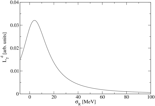
Figure 1: LIT L${}_{\gamma}^{d}$ with $\sigma_{I}$=10 MeV.

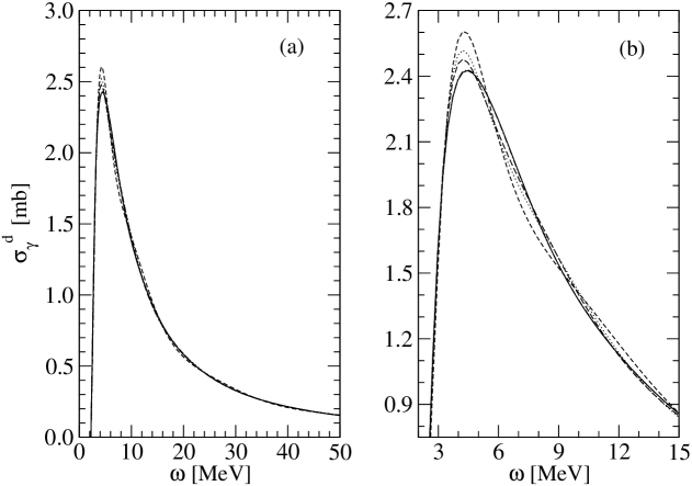
Figure 2: $\sigma_{\gamma}^{d}$ from inversion of L${}_{\gamma}^{d}$ of Fig. 1, up to 50 MeV (a) and in peak region (b), with various $M_{\rm max}$ values: 10 (short dashed), 15 (dotted), 20 (long dashed), 25 (solid), 26 (dash-dotted).

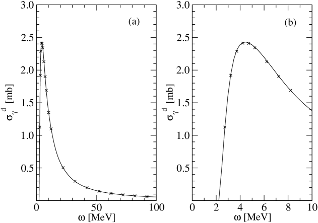
Figure 3: Total deuteron photoabsorption cross section up to 50 MeV (a) and in peak region (b): LIT result (solid) and from calculation with explicit $np$ continuum wave functions (crosses).

First we consider deuteron photodisintegration with a realistic NN interaction. In the already mentioned review article of the LIT method ELOB07 , such a case has been investigated using the AV14 NN potential AV14 . The L${}_{\gamma}^{d}$ result is shown in Fig. 1, while the corresponding inversion results are illustrated in Fig. 2. For the inversion one observes a nice stability range of the results for all the shown $M_{\rm max}$ values in the whole considered energy range, except for the peak region, where the inversion becomes stable only for higher $M_{\rm max}$. One notes that the $M_{\rm max}$ values 25 and 26 lead essentially to identical results.

In Fig. 3 the final inversion result ($M_{\rm max}$=25) is compared with the corresponding cross section of a conventional calculation with explicit $np$ continuum wave functions ELOB07 . One finds an excellent agreement between the two calculations showing that one can reach high-precision results with the LIT method.

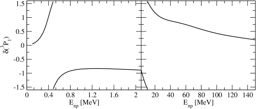
Figure 4: Phase shift ${}^{3}P_{1}$ of fictitious $np$ system at low (left) and higher (right) energies.

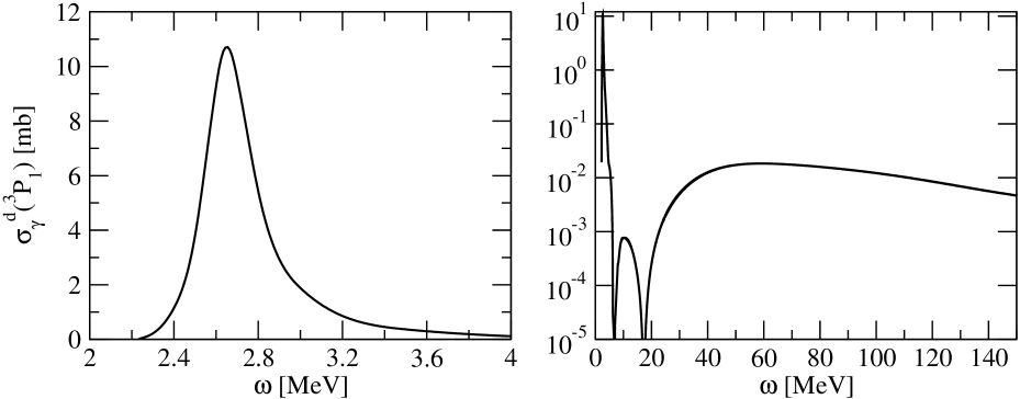
Figure 5: As Fig. 4 but for photodisintegration cross section.

Further LIT calculations for the deuteron total photoabsorption cross sections have already been discussed in JISP ; WL08 . For the aim of the present discussion, i.e. the way of working of the LIT method, WL08 is particularly interesting. It is a case study for a fictitious $np$ system with a low-lying and narrow resonance in the ${}^{3}P_{1}$ nucleon-nucleon partial wave (obtained by an additional attractive term, for details see WL08 ). The results of a conventional calculation with the fictitious $np$ system for the ${}^{3}P_{1}$ phase shifts and the “deuteron photoabsorption cross section” to the ${}^{3}P_{1}$ final state are shown in Figs. 4 and 5, respectively. The ${}^{3}P_{1}$ phase shifts exhibit two resonances, at $E_{np}=0.48$ MeV and at about $E_{np}=10.5$ MeV. The low-energy resonance leads to the dominant structure of the photoabsorption cross section, a pronounced peak at a photon energy of 2.65 MeV with a width $\Gamma$ of 270 keV, while the second resonance only shows up as a rather tiny peak, which is more than four orders of magnitude smaller than the first peak.

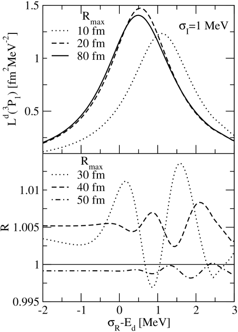
Figure 6: LIT L${}^{d}_{\gamma}(^{3}P_{1})$ of fictitious $np$ system in first resonance region with $\sigma_{I}=1$ MeV and various values of $R_{\rm max}$ (top) and ratio R=L${}^{d}_{\gamma}(R_{\rm max})/L^{d}_{\gamma}(R_{\rm max}=80$ fm) (bottom).

For the LIT calculation of the photoabsorption cross section of the fictitious $np$ system the inversion basis set $\chi_{m}$ (15) is modified to account for the resonant structure, to this end the functions $\chi_{m}$ are relabeled: $\chi_{m}\rightarrow\chi_{m+1}$. In addition a new $\chi_{1}$ is defined,

$$\chi_{1}(E_{np},\alpha_{i})={\frac{1}{(E_{np}-E_{\rm res})^{2}+({\frac{\Gamma}{2}})^{2}}}\left({\frac{1}{1+\exp(-1)}}-{\frac{1}{1+\exp((E_{np}-\alpha_{3})/\alpha_{3})}}\right)\,,$$ (29)

where $E_{\rm res}\equiv\alpha_{4}$, $\Gamma\equiv\alpha_{5}$ and $\alpha_{3}$ are additional nonlinear parameters.

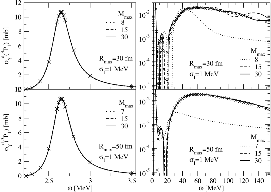
Figure 7: $\sigma^{d}_{\gamma}(^{3}P_{1})$ of fictitious $np$ system from inversion of L${}^{d}_{\gamma}(^{3}P_{1},\sigma_{I}=1$ MeV, $R_{\rm max})$ with various $M_{\rm max}$ values and $R_{\rm max}=30$ fm (top) and 50 fm (bottom) in first resonance region (left) and beyond (right); also shown results of a conventional calculation with explicit $np$ continuum wave functions (crosses).

The reason for such a LIT case study with a resonance lies in the results of a previous LIT calculation for the (e,e’) longitudinal and transverse form factors of ⁴He Sonia07 , where a resonance in the Coulomb monopole transition was obtained, but its width could not be determined. In the case study it is shown that for a proper resolution of a resonant structure it is very important to take into account the LIT function $\tilde{\Psi}$ up to rather large distances WL08 . This has been checked (i) by solving (6) imposing at a two-nucleon distance $r=R_{\rm max}$ an asymptotic boundary condition which leads to a strong fall-off of $\tilde{\Psi}(^{3}P_{1})$ and (ii) by calculating the norm $\langle\tilde{\Psi}(^{3}P_{1})|\tilde{\Psi}(^{3}P_{1})\rangle$ only in the range from $r=0$ to $r=R_{\rm max}$. In Fig. 6 we show the results for such a calculation choosing $\sigma_{I}=1$ MeV. One notes that for a rather precise result, with errors below about 1%, one has to take $R_{\rm max}\geq 30$ fm. A further increase of $R_{\rm max}$ to 50 fm leads to a reduction of the relative error by about a factor ten. In Fig. 7 the inversions results with $R_{\rm max}=30$ and 50 fm are depicted in comparison to the result of the direct calculation. One observes that for both $R_{\rm max}$ values the resonance cross section is described with high accuracy. Differences between the two cases become evident in the region of the second maximum and at higher energy. In fact with $R_{\rm max}=30$ fm one finds only a reasonably good description, while a considerable improvement is obtained with $R_{\rm max}=50$ fm.

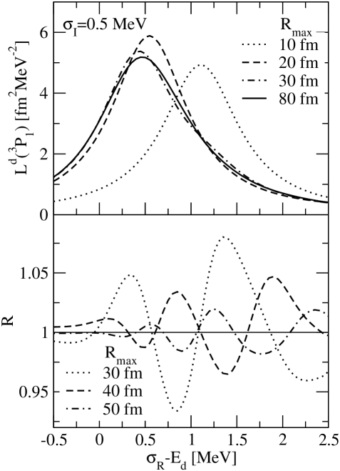
Figure 8: As Fig. 6 but with $\sigma_{I}=0.5$ MeV

As next point we consider the reduction of $\sigma_{I}$ from 1 MeV to 0.5 MeV. As shown in Fig. 8 one finds an enhancement of the relative error of $L_{\gamma}^{d}$ by at least a factor of five in comparison to the corresponding $R_{\rm max}$ values of Fig. 6. The enhancement is easily understood by investigating the asymptotic solution of (6); in the here considered deuteron case it is described by the exponential fall-off $\exp(-r(M\sigma_{I})^{\frac{1}{2}}/\hbar)$, where $M$ is the nucleon mass. It is evident that a smaller $\sigma_{I}$ leads to a longer range LIT function $\tilde{\Psi}$. As discussed in WL08 , for $\sigma_{I}=0.1$ MeV even $R_{\rm max}=$300 fm is not completely sufficient, since only the resonance itself is resolved, but not the cross section at higher energies.

The discussion above seems to infer that it is better to choose a rather large value for $\sigma_{I}$. On the other hand it should also be clear that the width of the resonance $\Gamma$ and the value of $\sigma_{I}$ are correlated. If $\sigma_{I}$ is too large the resonance cannot be resolved. In the case study it has been found that $\sigma_{I}=2$ MeV, about seven times larger than the width $\Gamma$, is still sufficient for a resolution of the resonance. However, in a general case the resonance width is not known beforehand and the question arises what should be the proper value for $\sigma_{I}$ in such a case. As pointed out in WL08 one has to proceed as follows. One performs a LIT calculation with a given $\sigma_{I}$ and compares the result to a LIT with a $\delta$-peak in the response function or cross section. For example, in the here discussed deuteron case one sets

$$R_{\gamma}^{\rm peak}(E_{np})=R^{\rm peak}\delta(E_{np}-E^{\rm peak})\,.$$

The resulting $\delta$-LIT is then given by the Lorentzian function

$${\rm L}^{d}_{\delta}(E^{\rm peak},\sigma_{R},\sigma_{I})=R^{\rm peak}{\mathcal{L}}(E^{\rm peak},\sigma_{R},\sigma_{I})\,,$$

where $R^{\rm peak}$ is chosen such that the peak heights of ${\rm L}^{d}_{\delta}$ and ${\rm L}^{d}_{\gamma}$ are equal.

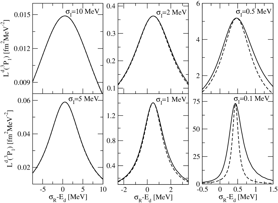
Figure 9: LIT L${}^{\rm d}(^{3}P_{1})$ (full curves) and L${}^{\rm d}_{\delta}$ (dashed curves) of fictitious $np$ system in first resonance region with various $\sigma_{I}$ values and $R_{\rm max}=80$ fm, except for $\sigma_{I}=0.1$ MeV where $R_{\rm max}$=300 fm.

In order to obtain a reliable inversion the actual LIT ${\rm L}^{d}_{\gamma}$ should have a larger width than the $\delta$-LIT ${\rm L}^{d}_{\delta}$. If, on the contrary, they lead to essentially identical results, one has to reduce $\sigma_{I}$ up to the point that the actual LIT is sufficiently different from the corresponding $\delta$-LIT. In Fig. 9 we show such results for the deuteron case study. For $\sigma_{I}$=5 and 10 MeV there are practically no differences between LIT and $\delta$-LIT, while for $\sigma_{I}\leq 2$ MeV differences become visible. As a matter of fact $\sigma_{I}$=2 MeV is sufficient for a reliable inversion and thus one may conclude that in a general case one has to use a $\sigma_{I}$ such that differences between LIT and $\delta$-LIT have at least the same size as in the $\sigma_{I}$=2 MeV case of Fig. 9.

In Fig. 10 we show the final inversion results from WL08 with $R_{\rm max}=$80 fm. One sees that the E1 resonance is precisely described with the LIT method for $\sigma_{I}=0.5$ and 2 MeV, while the peak is somewhat underestimated with $\sigma_{I}=5$ MeV. In the resonance region, with the two lower $\sigma_{I}$ values, essentially the same results are obtained as for the cases of Fig. 7 with $\sigma_{I}$=1 MeV and $R_{\rm max}=$30 and 50 fm. From the comparison one further notes that the case $\sigma_{I}$=2 MeV and $R_{\rm max}=80$ fm leads to even more precise results in the second resonance region, and beyond, than shown in Fig. 7 for $R_{\rm max}=$50 fm.

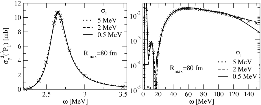
Figure 10: As Fig. 7 but with $R_{\rm max}=80$ fm and $\sigma_{I}=5$, 2, and 0.5 MeV.

V.2 Reactions with $A\geq 3$

Now we turn to realistic applications of the LIT method and consider first the ⁴He total photoabsorption cross section. In fact this is one of the very first LIT applications 4-body , however, initially only performed with semirealistic NN forces. In 4-body it has been found that the calculated cross section shows a considerably more pronounced giant dipole resonance than the most recent experimental data of that time. Such a difference between experiment and an ab initio calculation has led to a renewed experimental interest in the ⁴He photoabsorption cross section. In fact in the meantime three additional experiments have been carried out Nilsson ; Shima ; Nakayama . Finally, in Doron06 the first calculation with realistic NN and 3N forces has also been published. In Fig. 11 we show the theoretical results of Doron06 together with the experimental data. One notes that the 3N force leads to a considerable reduction of the peak cross section. One further sees that there is a very good agreement between theory and the data of Nakayama and also quite a good agreement with the data of Nilsson , while the cross section of Shima shows a completely different behavior. Also shown in the figure are data from experiments performed about 20 years ago.

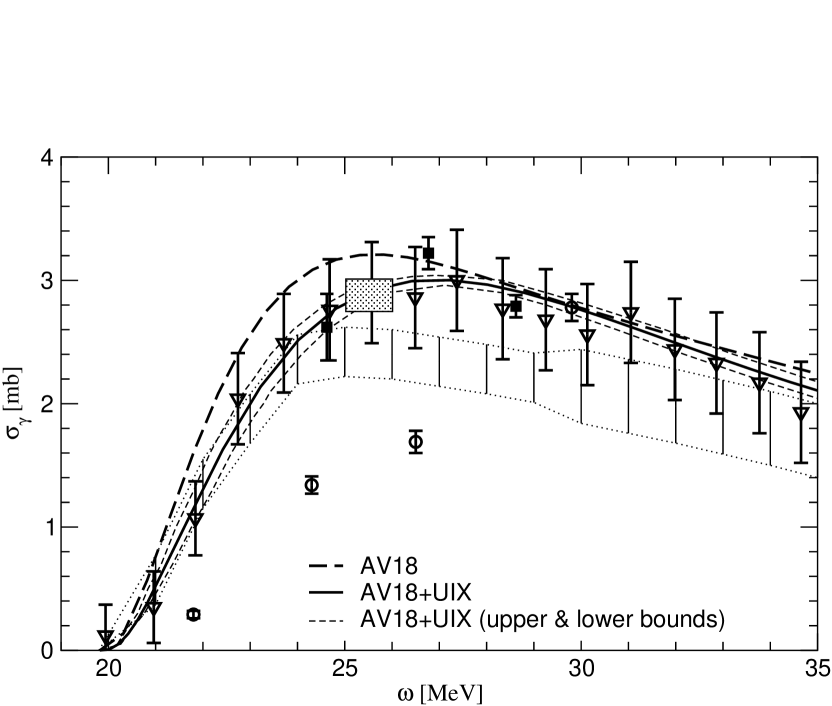
Figure 11: Total ⁴He photoabsorption cross section: LIT calculation with AV18 NN potential only AV18 , and with additional UIX 3N force UIX ; experimental data: squares Nilsson , circles Shima , triangles Nakayama , area between dotted lines Berman ; Feldman , and dotted box Wells .

It should be mentioned that today two other LIT calculations for the ⁴He total photoabsorption cross section are available Sonia_UCOM ; Sofia_NCSM , where different realistic nuclear forces have been used. Essentially, they confirm the results of Doron06 .

In Fig. 12 LIT results for the ⁶Li and ⁶He total photoabsorption cross sections calculated with semirealistic NN forces are shown 6-body . For ⁶Li one finds a single and rather broad cross section peak. On the contrary for ⁶He a very interesting cross section with a double peak becomes apparent in the calculation. This microscopic result can be interpreted as follows. In a cluster picture, with an $\alpha$ core and a di-neutron, the low-energy peak is due to the relative motion of di-neutron and $\alpha$ core. The second peak, however, cannot be obtained in a cluster model, but is explained by the classical E1 giant resonance picture with a collective response of all nucleons (relative motion of protons and neutrons). For ⁶Li, in a cluster model described by an $\alpha$ core plus a deuteron, a similar low-energy peak is missing, because the deuteron knock-out corresponds to an isoscalar transition, which cannot be induced by the isovector dipole operator (27). On the other hand a transition to the antibound ${}^{1}S_{0}(np)$ plus $\alpha$ core is possible. The nucleus ⁶Li exhibits a considerably larger width of the giant dipole peak than ⁶He. In fact in the former a break-up into two three-body nuclei is possible (³H$-^{3}$He), while a similar break-up of ⁶He is not induced by the dipole operator, since the ³H$-^{3}$H pair has no dipole moment. The experimental ⁶He and ⁶Li photoabsorption cross sections are not yet well settled (see 6-body ) and therefore not shown here.

Figure 12: ⁶Li and ⁶He total photoabsorption cross sections with various semirealistic NN potential models: AV4’ AV4' , MN MN , and MTI-III MT .

Figure 13: ⁷Li total photoabsorption cross section with semirealistic NN potential model AV4’, experimental data from Ahrens .

In Fig. 13 we depict the LIT calculation for the ⁷Li total photoabsorption cross section 7-body , in comparison to experimental data Ahrens . It is worthwhile to mention that the experimental cross section has not been determined by summing up the various channel cross sections, but in a single experiment by the “diminution of photon flux” method. Like ⁶Li also ⁷Li has a giant dipole resonance peak with a rather large width. The comparison of experimental and theoretical results shows quite a good agreement, though only a semirealistic NN force has been used in the LIT calculation. Of course, it would be very interesting to have even more precise data and also a calculation with realistic nuclear forces.

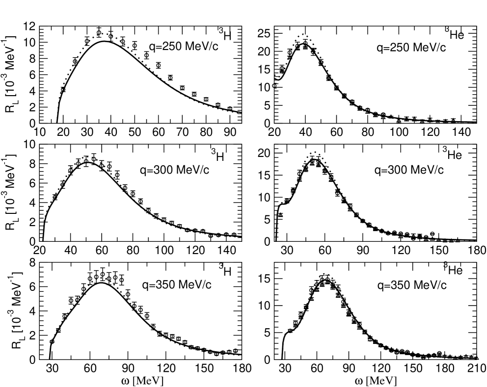
Figure 14: $R_{L}(\omega,q)$ of ³H (left) and ³He (right) at various $q$: AV18 NN potential (dotted), AV18 NN + UIX 3N potential (solid); experimental data: triangles Saclay , and circles Bates .

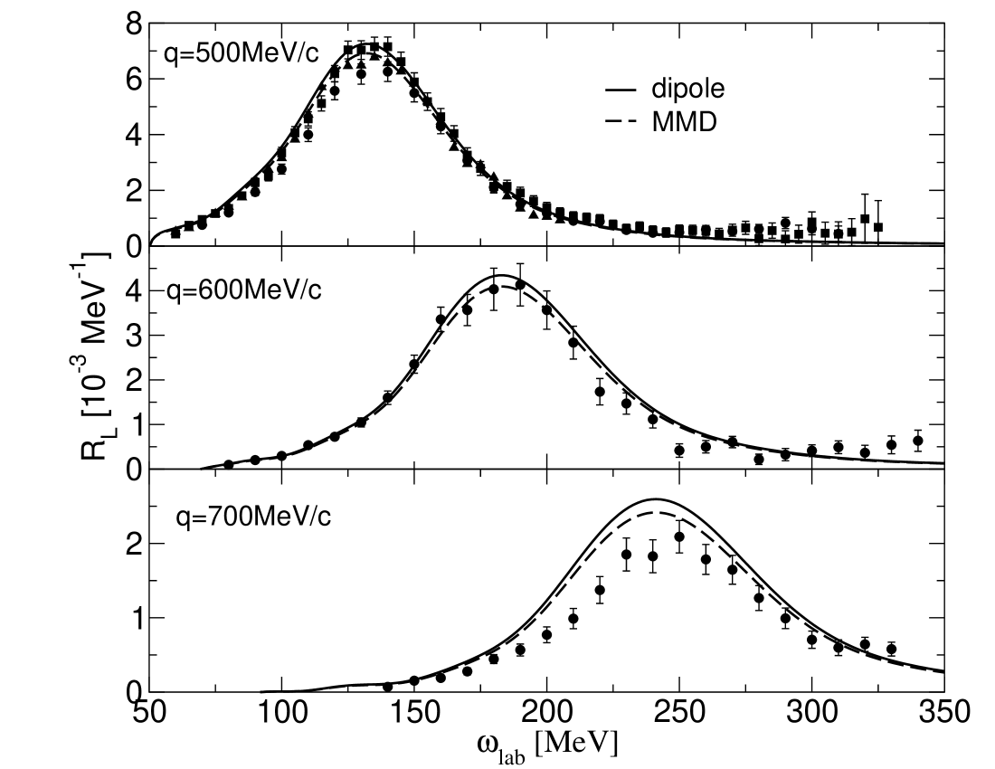
Figure 15: $R_{L}(\omega,q)$ of ³He at various $q$, calculation with AV18 NN + UIX 3N potentials and two nucleon form factors fits: dipole (solid) and MMD from MMD (dashed); experimental data: squares Saclay , triangles Bates , and circles world .

Now we turn to the inclusive electron scattering response functions. For ³H and ³He LIT calculations for the longitudinal response function $R_{L}(\omega,q)$ have been carried out with realistic nuclear forces for momentum transfers below ee'04 , and above $q$=500 MeV/c ee'05 . Relativistic corrections for the transition operator $O_{L}$ have been taken into account and the frame dependence of the essentially nonrelativistic calculation has been studied. In Fig. 14 $R_{L}$ is shown for various lower $q$ values ee'04 . One notes that the 3N force reduces the quasielastic peak height somewhat. The 3N force effect, however, does not lead to a consistent picture in comparison with experiment. In fact one finds an improvement for ³He and a deterioration for ³H.

In ee'05 it has been found that relativistic effects due to the kinetic energy can be largely reduced if $R_{L}$ is first calculated in a specific reference frame, where the target nucleus moves with –A${\bf q}/2$, and then transformed to the lab system. Different from a direct calculation in the lab system, one finds a correct result for the experimentally established quasielastic peak position ee'05 , as shown in Fig. 15. At $q$=500 and 600 MeV/c also for the peak height a good agreement with experimental data is obtained, whereas the theoretical $R_{L}$ overestimates the experimental one at $q$=700 MeV/c (at even higher $q$ experimental data are not available). As Fig. 15 shows also the choice of the nucleon form factor fit has a non-negligible impact on the result, but cannot explain the discrepancy with the data at $q=700$ MeV/c.

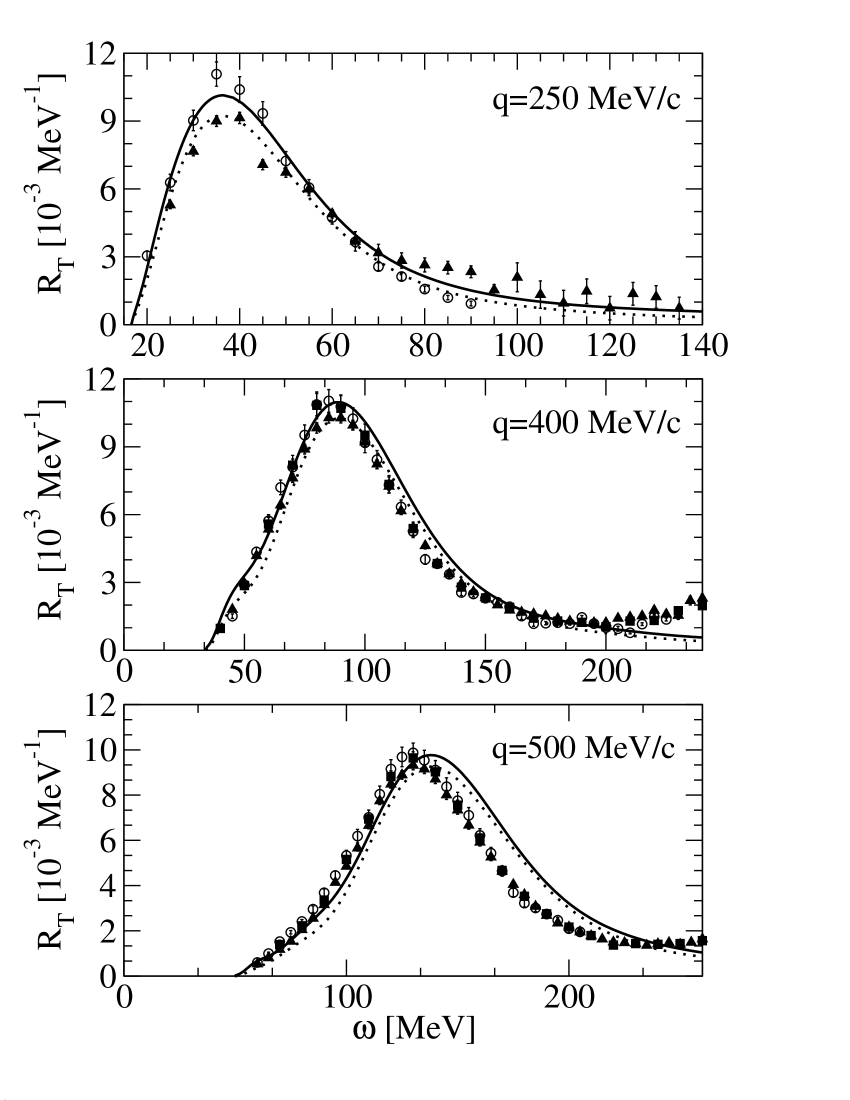
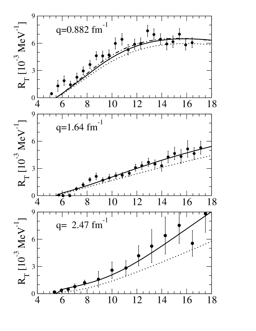
Figure 16: $R_{T}(\omega,q)$ in quasielastic (left) and threshold region (right), theoretical results with BonnRA NN potential Bonn , and TM’ 3N forces TM , and following current operators: one-body (dotted) and one-body + $\pi$-EC + $\rho$-EC + additional EC via Siegert operator (solid). Experimental data: left panels, triangles Saclay , circles Bates , and squares world ; and right panels, circles Retzlaff .

Recently we also calculated the transverse response function $R_{T}(\omega,q)$ with realistic nuclear forces ($q\leq 500$ MeV/c) ee'08 . Besides the usual one-body operators also $\pi$ and $\rho$ exchange currents (EC), consistent with the NN potential model, were taken into account. In addition also the effect of the so-called Siegert operator has been studied. In Fig. 16 the theoretical results are shown together with experimental data. In the quasielastic region EC lead to some increase of the peak height (see left panels of Fig. 16), but the EC effect is much larger close to threshold (see right panels of Fig. 16) and is important for a good agreement of theory and experiment. For $q$=500 MeV/c one finds different peak positions in theory and experiment, presumably due to the fact that $R_{T}$ is calculated directly in the lab frame (see discussion above). The frame dependence of $R_{T}$ is presently under investigation.

Presently we are extending our realistic calculation to the $(e,e^{\prime})$ response functions of ⁴He and results for $R_{L}$ will be published soon.

Summarizing one may conclude that the LIT method is very powerful and allows a considerable extension of the range of microscopic ab initio calculations.

References

- (1) V. D. Efros, W. Leidemann, and G. Orlandini, Phys. Lett. B338, 130 (1994).
- (2) V. D. Efros, Yad. Fiz. 41, 1498 (1985) [Sov. J. Nucl. Phys. 41, 949 (1985)].
- (3) V. D. Efros, W. Leidemann, and G. Orlandini, Few-Body Syst. 14, 151 (1993).
- (4) V. D. Efros, W. Leidemann, G. Orlandini, and E. L. Tomusiak, Phys. Lett. B484, 223 (2000).
- (5) D. Gazit et al., Phys. Rev. Lett. 96, 112301 (2006).
- (6) D. Gazit and N. Barnea, Phys. Rev. Lett. 98, 192501 (2007).
- (7) V. D. Efros, W. Leidemann, and G. Orlandini, Phys. Rev. Lett. 78, 4015 (1997); N. Barnea, V. D. Efros, W. Leidemann, and G. Orlandini, Phys. Rev. C63, 057002 (2001).
- (8) S. Bacca et al., Phys. Rev. Lett. 89, 052502 (2002); S. Bacca, N. Barnea, W. Leidemann, and G. Orlandini, Phys. Rev. C69, 057001 (2004).
- (9) S. Bacca et al., Phys. Lett. B603, 159 (2004).
- (10) V. D. Efros, W. Leidemann, and G. Orlandini, Phys. Rev. Lett. 78, 432 (1997).
- (11) V. D. Efros, W. Leidemann, G. Orlandini, and E. L. Tomusiak, Phys. Rev. C72, 011002(R) (2005).
- (12) S. Della Monaca et al., Phys. Rev. C77, 044007 (2008).
- (13) S. Quaglioni et al., Phys. Rev. C69, 044002 (2004).
- (14) S. Quaglioni, V. D. Efros, W. Leidemann, and G. Orlandini, Phys. Rev. C72, 064002 (2005).
- (15) D. Andreasi et al., Eur. Phys. J. A27, 47 (2006).
- (16) V. D. Efros, W. Leidemann, G. Orlandini, and N. Barnea, J. Phys. G34, R459 (2007).
- (17) J. D. Walecka, Theoretical Nuclear and Subnuclear Physics (World Scientific, Singapore, 2004).
- (18) H. Arenhövel, W. Leidemann, and E. L. Tomusiak, Eur. Phys. J. A23, 147 (2005).
- (19) D. Andreasi, W. Leidemann, Ch. Reiss, and M. Schwamb, Eur. Phys. J. A24, 361 (2005).
- (20) M. L. Goldberger and K. W. Watson, Collision Theory (Wiley, New York, 1964).
- (21) A. La Piana and W. Leidemann, Nucl. Phys. A677, 423 (2000).
- (22) Yu. I. Fenin and V. D. Efros, Yad. Fiz. 15, 887 (1972) [Sov. J. Nucl. Phys. 15, 497 (1972)]; W. Leidemann, V. D. Efros, G. Orlandini, and E. L. Tomusiak, Fizika B8, 135 (1999).
- (23) N. Barnea, W. Leidemann, and G. Orlandini, Phys. Rev. C61, 054001 (2000); N. Barnea, W. Leidemann, and G. Orlandini, Nucl. Phys. A693, 565 (2001).
- (24) M. Marchisio, N. Barnea, W. Leidemann, and G. Orlandini, Few-Body Syst. 33, 259 (2003).
- (25) R. B. Wiringa, R. A. Smith, and T. L. Ainsworth, Phys. Rev. C29, 1207 (1984).
- (26) N. Barnea, W. Leidemann, and G. Orlandini, Phys. Rev. C74, 034003 (2006).
- (27) W. Leidemann, Few-Body Syst. in print, arXiv:0803.1770.
- (28) S. Bacca et al. Phys. Rev. C76, 014003 (2007).
- (29) B. Nilsson et al., Phys. Lett. B626, 65 (2005).
- (30) T. Shima et al., Phys. Rev. C72, 044004 (2005).
- (31) S. Nakayama et al., Phys. Rev. C76, 021305(R) (2007).
- (32) R. B. Wiringa, V. G. J. Stoks, and R. Schiavilla, Phys. Rev. C51, 38 (1995).
- (33) B. S. Pudliner et al., Phys. Rev. C56, 1720 (1997).
- (34) B. L. Berman, D. D. Faul, P. Meyer, and D. L. Olson, Phys. Rev. C22, 2273 (1980).
- (35) G. Feldman et al., Phys. Rev. C42, R1167 (1990).
- (36) D. P. Wells et al., Phys. Rev. C46, 449 (1992).
- (37) S. Bacca, Phys. Rev. C75, 044001 (2007).
- (38) S. Quaglioni and P. Navràtil, Phys.Lett. B652, 370 (2007).
- (39) R. B. Wiringa and S. C. Pieper, Phys. Rev. Lett. 89, 182501 (2002).
- (40) D. R. Thomson, M. LeMere, and Y. C. Tang, Nucl. Phys. A286, 53 (1977); I. Reichstein and Y. C. Tang, ibid. A158, 529 (1970).
- (41) R. A. Malfliet and J. Tjon, Nucl. Phys. A127, 161 (1969).
- (42) J. Ahrens et al., Nucl. Phys. A251, 479 (1975).
- (43) V. D. Efros, W. Leidemann, G. Orlandini, and E. L. Tomusiak, Phys. Rev. C69, 044001 (2004).
- (44) C. Marchand et al., Phys. Lett. B153, 29 (1985).
- (45) K. Dow et al., Phys. Rev. Lett. 61, 1706 (1988).
- (46) J. Carlson, J. Jourdan, R. Schiavilla, and I. Sick, Phys. Rev. C65, 024002 (2002).
- (47) P. Mergell, U.-G. Meissner, and D. Drechsel, Nucl. Phys. A596, 367 (1996).
- (48) R. Machleidt, Adv. Nucl. Phys. 19, 189 (1989).
- (49) S. A. Coon et al., Nucl. Phys. A317, 242 (1979).
- (50) G. A. Retzlaff et al., Phys. Rev. C49, 1263 (1994).