Atomic spin squeezing in an optical cavity

Abstract

We consider squeezing of one component of the collective spin vector of an atomic ensemble inside an optical cavity. The atoms interact with a cavity mode, and the squeezing is obtained by probing the state of the light field that is transmitted through the cavity. Starting from the stochastic master equation, we derive the time evolution of the state of the atoms and the cavity field, and we compute expectation values and variances of the atomic spin components and the quadratures of the cavity mode. The performance of the setup is compared to spin squeezing of atoms by probing of a light field transmitted only once through the sample.

I Introduction

Interactions between light and matter have several applications within quantum information processing. When a light field interacts with a collection of atoms, the light and the atoms become entangled, and the state of the total system can no longer be written as a direct product of quantum states of the individual systems. As a consequence, if the light field is subsequently subjected to measurements, the state of the atoms will also be affected. This has, for instance, been utilized to entangle two atomic ensembles duan ; julsgaard and to teleport the state of a light field onto atoms teleportation . It has also been suggested to generate various squeezed and entangled states of light and matter by sending a light field twice sherson2 or multiple times hammerer through the same atomic ensemble from different directions.

The generation of entanglement between light and atoms may also be utilized to perform a quantum nondemolition measurement of one of the components of the collective spin vector of an atomic ensemble kuzmich ; takahashi ; kuzmichexp ; thomsen ; geremia ; hammerer ; madsen ; sherson . The measurements can reduce the uncertainty in the measured observable below the uncertainty of a coherent spin state, resulting in a squeezed spin state. Apart from the fundamental interest in generating squeezed states, spin squeezing can improve the precision of measurements of, for instance, weak magnetic fields budker ; partner . The strength of the interaction between light and atoms is normally weak but can be enhanced by placing the atoms inside an optical cavity as depicted in Fig. 1, and in the present paper we investigate the performance of spin squeezing in a cavity compared to spin squeezing in free space.

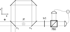
Figure 1: Experimental setup for probing of the $z$-component of the collective spin of an atomic ensemble with electromagnetic radiation. A continuous laser beam linearly polarized in the $x$-direction and with photon flux $\Phi$ enters the cavity from the left. The interaction between the light and the atoms, described by the Hamiltonian $H$, rotates the polarization vector of the light field by an amount, which depends on the $z$-component of the atomic spin. The angle of rotation can be measured by performing a detection on the light leaking out of the cavity ($\kappa_{1}$ and $\kappa_{2}$ denote cavity decay rates). The half wave plate transforms the field operators $\hat{a}_{x}$ and $\hat{a}_{y}$ for $x$- and $y$-polarized light into $(\hat{a}_{x}+\hat{a}_{y})/\sqrt{2}$ and $(\hat{a}_{x}-\hat{a}_{y})/\sqrt{2}$, and these polarization components are subsequently separated by the polarizing beam splitter (PBS). The measurement outcome is the difference in photo current between the two photo detectors.

In spin squeezing experiments the usual initial state of the atoms is a coherent spin state, where all the atomic spins are oriented in the same direction, which we shall take as the $x$-direction. If the number of atoms is large, the $x$-component of the collective atomic spin $\hat{\bm{J}}=\sum_{i}\hat{\bm{j}}_{i}$, where $\hat{\bm{j}}_{i}$ is the total spin of the $i$th atom, may be treated as a classical quantity $\hat{J}_{x}\approx\langle\hat{J}_{x}\rangle$, and the commutator between the scaled spin components $\hat{x}_{\textrm{at}}=\hat{J}_{y}/(\hbar\langle\hat{J}_{x}\rangle)^{1/2}$ and $\hat{p}_{\textrm{at}}=\hat{J}_{z}/(\hbar\langle\hat{J}_{x}\rangle)^{1/2}$ turns into the canonical commutator $[\hat{x}_{\textrm{at}},\hat{p}_{\textrm{at}}]=i$. In this approximation the initial coherent spin state is a Gaussian state, and since the interaction Hamiltonian and the measurements transform Gaussian states into Gaussian states as long as $\hat{J}_{x}$ can be treated classically, a very efficient Gaussian formalism, which provides several analytical results for both pulsed and continuous wave fields, is applicable, as demonstrated for free fields in Refs. madsen ; sherson . The Gaussian description is easily generalized to take an optical cavity into account nm4 , but although we shall be mainly concerned with the limit of a large number of atoms below, we also demonstrate that analytical results can be obtained even without assuming the Gaussian approximation for the collective atomic spin.

The paper is structured as follows. In Sec. II we apply the stochastic master equation for the setup in Fig. 1 to derive expressions for the time evolution of the state of the atoms and the cavity field, and in Sec. III we evaluate the variances and mean values of the collective atomic spin operators and the quadratures of the cavity field as a function of time in the limit of a large number of atoms. Effects of losses due to spontaneous decay is considered in Sec. IV, and the results are compared to those obtained for squeezing in free space. Section V concludes the paper.

II Atoms interacting with off-resonant light in a cavity

We consider atoms with a spin $1/2$ ground state $|g_{\mp}\rangle$ and a spin $1/2$ excited state $|e_{\mp}\rangle$ interacting with a strong, off-resonant cavity field, which is initially linearly polarized in the $x$-direction. Decomposing the light into right and left circularly polarized cavity modes with field annihilation operators $\hat{a}_{+}=(-\hat{a}_{x}+i\hat{a}_{y})/\sqrt{2}$ and $\hat{a}_{-}=(\hat{a}_{x}+i\hat{a}_{y})/\sqrt{2}$, respectively, the Hamiltonian takes the form

$$H=\hbar g\sum_{i=1}^{N_{\textrm{at}}}\left(\hat{a}_{+}|e_{+,i}\rangle\langle g_{-,i}|+\hat{a}_{-}|e_{-,i}\rangle\langle g_{+,i}|+\textrm{h.c.}\right)\\ -\hbar\Delta\sum_{i=1}^{N_{\textrm{at}}}\left(|e_{+,i}\rangle\langle e_{+,i}|+|e_{-,i}\rangle\langle e_{-,i}|\right)$$ (1)

in a frame rotating with the frequency of the light field. The summation runs over the $N_{\textrm{at}}$ atoms, $\hbar g=-dE_{0}$, $d$ is the atomic dipole moment, $E_{0}=\sqrt{\hbar\omega/(V\epsilon_{0})}$, $\omega$ is the angular frequency of the light field, $V$ is the mode volume, $\epsilon_{0}$ is the vacuum permittivity, and $\Delta=\omega-\omega_{\textrm{at}}$ is the detuning between the light field and the atomic transition. For sufficiently large detuning $g/\Delta\ll 1$, the excited states will not become significantly populated and can be adiabatically eliminated, which leads to the effective Hamiltonian

$$H=\frac{\hbar g^{2}}{\Delta}\sum_{i=1}^{N_{\textrm{at}}}\left(\hat{a}_{+}^{\dagger}\hat{a}_{+}|g_{-,i}\rangle\langle g_{-,i}|+\hat{a}_{-}^{\dagger}\hat{a}_{-}|g_{+,i}\rangle\langle g_{+,i}|\right).$$ (2)

In this and the next section, we neglect loss of photons and atomic coherence due to spontaneous emission from the excited states, but we return to an analysis of the role of spontaneous atomic emission of light in Sec. IV. Since $\sum_{i}|g_{\mp,i}\rangle\langle g_{\mp,i}|=N_{\textrm{at}}/2\pm\hat{J}_{z}/\hbar$,

$$H=\frac{\hbar g^{2}}{\Delta}\frac{N_{\textrm{at}}}{2}(\hat{a}_{x}^{\dagger}\hat{a}_{x}+\hat{a}_{y}^{\dagger}\hat{a}_{y})-i\frac{\hbar g^{2}}{\Delta}\left(\hat{a}_{x}^{\dagger}\hat{a}_{y}-\hat{a}_{y}^{\dagger}\hat{a}_{x}\right)\frac{\hat{J}_{z}}{\hbar}.$$ (3)

The first term gives rise to a common phase shift of the $x$- and $y$-polarized light and can be compensated by introducing an additional phase shift in the cavity, for instance by adjusting the length of the cavity. We thus ignore this term in the following. For the setup depicted in Fig. 1, it is desirable to have a large number of photons in the $x$-polarized mode, since this increases the strength of the light-atom interaction, and since, in the polarization rotation measurement, the $x$-polarized field acts the same way as a local oscillator in balanced homodyne detection. Approximating $\hat{a}_{x}$ by its expectation value $\langle\hat{a}_{x}(t)\rangle$, the infinitesimal time evolution operator corresponding to the second term in (3) takes the form $\hat{U}=\exp\left((g^{2}/\Delta)\left(\langle\hat{a}_{x}(t)\rangle\hat{a}_{y}^{\dagger}-\langle\hat{a}_{x}^{\dagger}(t)\rangle\hat{a}_{y}\right)(\hat{J}_{z}/\hbar)dt\right)$, and comparing this to the displacement operator $\hat{D}(\delta)=\exp(\delta\hat{a}_{y}^{\dagger}-\delta^{*}\hat{a}_{y})$, we observe that the interaction displaces the $y$-polarized field amplitude by an amount, which is proportional to the $z$-component of the atomic spin. Detecting the quadrature of the $y$-polarized field in the direction of the displacement thus constitutes an indirect measurement of $\hat{J}_{z}$ as stated above.

Assuming a high finesse cavity $\kappa\tau\ll 1$, where $\kappa$ is the total cavity decay rate and $\tau$ is the round trip time of light in the cavity, and an only infinitesimal change of the atomic quantum state on the time scale of $\tau$, we deduce from the detailed derivation in nm6 that the density operator $\rho(t)$, describing the state of the atoms and the $x$- and $y$-polarized cavity fields, satisfies the linearized stochastic master equation

$$d\rho(t)=-\frac{i}{\hbar}\left[H,\rho(t)\right]dt+\sqrt{\eta_{d}\kappa_{2}}\left(\hat{a}_{y}\rho(t)dt+\rho(t)\hat{a}_{y}^{\dagger}\right)dy_{s}\\ +\frac{\kappa}{2}\left(-\hat{a}^{\dagger}_{y}\hat{a}_{y}\rho(t)-\rho(t)\hat{a}^{\dagger}_{y}\hat{a}_{y}+2\hat{a}_{y}\rho(t)\hat{a}_{y}^{\dagger}\right)dt\\ +\frac{\kappa}{2}\left(-\hat{a}^{\dagger}_{x}\hat{a}_{x}\rho(t)-\rho(t)\hat{a}^{\dagger}_{x}\hat{a}_{x}+2\hat{a}_{x}\rho(t)\hat{a}_{x}^{\dagger}\right)dt\\ +\sqrt{\kappa_{1}}\beta(t)[\hat{a}_{x}^{\dagger},\rho(t)]dt-\sqrt{\kappa_{1}}\beta^{*}(t)[\hat{a}_{x},\rho(t)]dt,$$ (4)

where $\kappa=\kappa_{1}+\kappa_{2}+\kappa_{L}$, $\kappa_{1}$ ($\kappa_{2}$) is the cavity decay rate due to the lower left (right) cavity mirror in Fig. 1, $\kappa_{L}$ is the cavity decay rate due to additional losses, $\beta(t)$ is the amplitude of the incoming probe beam, $\eta_{d}$ is the detector efficiency, and $dy_{s}$ is a stochastic variable representing the measured difference in photo current at time $t$ (see nm6 for details). The first term in (4) is the Hamiltonian evolution due to the interaction between the atoms and the cavity modes, the second term represents the knowledge obtained from the continuous measurement, the third and fourth terms take cavity decay into account, and the fifth and sixth terms appear due to the presence of the input beam. The derivation in nm6 assumes that $\sqrt{\kappa_{1}}|\beta(t)|\tau$ is small, but, for a classical $x$-polarized mode, it is sufficient to assume that $\sqrt{\kappa_{1}}\beta(t)$ varies slowly within times of order $\tau$ (and if we are not interested in features of the solution occurring on a time scale $\tau$ or faster, we may even allow $\sqrt{\kappa_{1}}\beta(t)$ to change abruptly). In fact, if the $x$-polarized light is used as local oscillator as in Fig. 1, it is required that $4\kappa_{1}\kappa_{2}|\beta(t)|^{2}\tau/\kappa^{2}\gg 1$, since the local oscillator is assumed to be strong. We note that the stochastic term in (4) does not conserve the trace of the density operator, which should hence be normalized explicitly. The probability to obtain the normalized state $\rho(t+dt)/\textrm{Tr}(\rho(t+dt))$ at time $t+dt$, given that the normalized state at time $t$ was $\rho(t)$, is $\textrm{Tr}(\rho(t+dt))$ multiplied by the probability to obtain the required value of $dy_{s}$, assuming that $dy_{s}$ is a Gaussian distributed stochastic variable with zero mean value and variance $dt$. If it is the reflected light and not the transmitted light, which is subjected to measurement, and if the lower right cavity mirror in Fig. 1 is perfectly reflecting, we note that $\eta_{d}\kappa_{2}$ should be replaced by $\eta_{d}\kappa_{1}$ and $\kappa=\kappa_{1}+\kappa_{2}+\kappa_{L}$ should be replaced by $\kappa=\kappa_{1}+\kappa_{L}$ in Eq. (4).

Since the Hamiltonian (3) commutes with $\hat{\bm{J}}^{2}$, we can restrict ourselves to the basis consisting of the states with total spin quantum number $J=N_{\textrm{at}}/2$ if the initial state is a coherent spin state. We thus consider the states $J_{z}|n\rangle=\hbar n|n\rangle$ with $n=-N_{\textrm{at}}/2,-N_{\textrm{at}}/2+1,\ldots,N_{\textrm{at}}/2$, and write the density matrix as

$$\rho(t)=\sum_{n}\sum_{m}\rho_{nm}|n\rangle\langle m|,$$ (5)

where $\rho_{nm}$ are operators on the space of the $x$- and $y$-polarized cavity field modes. This leads to the $(N_{\textrm{at}}+1)^{2}$ independent equations

$$d\rho_{nm}=-\frac{g^{2}}{\Delta}n(\hat{a}_{x}^{\dagger}\hat{a}_{y}-\hat{a}_{y}^{\dagger}\hat{a}_{x})\rho_{nm}dt\\ +\frac{g^{2}}{\Delta}m\rho_{nm}(\hat{a}_{x}^{\dagger}\hat{a}_{y}-\hat{a}_{y}^{\dagger}\hat{a}_{x})dt\\ +\sqrt{\eta_{d}\kappa_{2}}(\hat{a}_{y}\rho_{nm}+\rho_{nm}\hat{a}_{y}^{\dagger})dy_{s}\\ +\frac{\kappa}{2}\left(-\hat{a}_{y}^{\dagger}\hat{a}_{y}\rho_{nm}-\rho_{nm}\hat{a}^{\dagger}_{y}\hat{a}_{y}+2\hat{a}_{y}\rho_{nm}\hat{a}_{y}^{\dagger}\right)dt\\ +\frac{\kappa}{2}\left(-\hat{a}_{x}^{\dagger}\hat{a}_{x}\rho_{nm}-\rho_{nm}\hat{a}^{\dagger}_{x}\hat{a}_{x}+2\hat{a}_{x}\rho_{nm}\hat{a}_{x}^{\dagger}\right)dt\\ +\sqrt{\kappa_{1}}\beta(t)[\hat{a}_{x}^{\dagger},\rho_{nm}]dt-\sqrt{\kappa_{1}}\beta^{*}(t)[\hat{a}_{x},\rho_{nm}]dt$$ (6)

with solution

$$\rho_{nm}=C_{nm}(t)|\gamma_{n}(t)\rangle_{x}\langle\gamma_{m}(t)|\otimes|\alpha_{n}(t)\rangle_{y}\langle\alpha_{m}(t)|,$$ (7)

where $|\gamma_{n}(t)\rangle$ and $|\alpha_{n}(t)\rangle$ are coherent states satisfying

$$\frac{d\gamma_{n}(t)}{dt}=-\frac{\kappa}{2}\gamma_{n}(t)-n\frac{g^{2}}{\Delta}\alpha_{n}(t)+\sqrt{\kappa_{1}}\beta(t)$$ (8)

and

$$\frac{d\alpha_{n}(t)}{dt}=-\frac{\kappa}{2}\alpha_{n}(t)+n\frac{g^{2}}{\Delta}\gamma_{n}(t).$$ (9)

For a classical input field the term in (8) proportional to $\alpha_{n}(t)$ is negligible, and, assuming $\beta(t)=\beta^{*}(t)=\sqrt{\Phi(t)}$ and $\alpha_{n}(0)=\gamma_{n}(0)=0$, we obtain

$$\langle\hat{a}_{x}(t)\rangle=\gamma_{n}(t)=\sqrt{\kappa_{1}}\int_{0}^{t}e^{-\kappa(t-t^{\prime})/2}\beta(t^{\prime})dt^{\prime}$$ (10)

and

$$\alpha_{n}(t)=n\frac{g^{2}}{\Delta}\int_{0}^{t}e^{-\kappa(t-t^{\prime})/2}\langle\hat{a}_{x}(t^{\prime})\rangle dt^{\prime}\equiv n\alpha(t),$$ (11)

where $\alpha(t)$ is real and independent of $n$. Under these conditions the coefficients $C_{nm}$ in (7) satisfy

$$\frac{dC_{nm}}{C_{nm}}=\sqrt{\eta_{d}\kappa_{2}}(n+m)\alpha(t)dy_{s}-\frac{\kappa}{2}(n-m)^{2}\alpha(t)^{2}dt$$ (12)

with solution

$$C_{nm}(t)=C_{nm}(0)\exp\bigg{(}-\frac{\kappa}{2}(n-m)^{2}\int_{0}^{t}\alpha(t^{\prime})^{2}dt^{\prime}\\ +\sqrt{\eta_{d}\kappa_{2}}(n+m)\int_{0}^{t}\alpha(t^{\prime})dy_{s}^{\prime}\\ -\frac{\eta_{d}\kappa_{2}}{2}(n+m)^{2}\int_{0}^{t}\alpha(t^{\prime})^{2}dt^{\prime}\bigg{)}.$$ (13)

If required, the analysis is easily generalized to include all simultaneous eigenstates of $\hat{\bm{J}}^{2}$ and $\hat{J}_{z}$, since it is only needed to include more terms in (5) and to introduce additional labels to distinguish the different states.

We finally note that if $\Phi(t)$ is zero for $t<0$ and assumes the constant value $\Phi$ for $t>0$ and if the light-atom coupling is sufficiently weak to ensure that the change in the state of the atoms during the transient is negligible, we may approximate $\langle\hat{a}_{x}(t)\rangle$ and $\alpha(t)$ by their respective steady state values $\langle\hat{a}_{x}\rangle=2\sqrt{\kappa_{1}\Phi}/\kappa$ and $\alpha=2g^{2}\langle\hat{a}_{x}\rangle/(\kappa\Delta)$ for $t>0$, which makes the integrals in (13) trivial to evaluate. In that case the state at time $t$ depends on the measurement result through the integrated signal $Y_{s}=\int_{0}^{t}dy_{s}$ only, and the probability density to measure a given value of $Y_{s}$ is nm6

$$P=\sum_{n}\frac{C_{nn}(0)}{\sqrt{2\pi t}}\exp\left(-\frac{(Y_{s}-2\sqrt{\eta_{d}\kappa_{2}}n\alpha t)^{2}}{2t}\right).$$ (14)

The measurement leads to a narrowing of the distribution $C_{nn}(t)/\sum_{m}C_{mm}(t)$ over the possible eigenstates of $\hat{J}_{z}$, but the expectation value of $\hat{J}_{z}$ depends on $Y_{s}$, and if we average over all possible measurement outcomes, we find that $C_{nn}(t)=C_{nn}(0)$.

III Expectation values of atomic spin operators for large $N_{\textrm{at}}$

Having obtained the state of the atoms and the $y$-polarized cavity field as a function of time, we can now evaluate expectation values and variances of the atomic spin operators and the field quadrature operators $\hat{x}_{\textrm{ph}}=(\hat{a}_{y}+\hat{a}_{y}^{\dagger})/\sqrt{2}$ and $\hat{p}_{\textrm{ph}}=-i(\hat{a}_{y}-\hat{a}_{y}^{\dagger})/\sqrt{2}$. We assume below that the initial state is a coherent spin state pointing in the $x$-direction and that the number of atoms is large $N_{\textrm{at}}\gg 1$, since this is a typical experimental condition, and since it allows us to simplify the obtained expressions considerably. In order to stay within the parameter regime where the Gaussian approximation, discussed in the Introduction, is valid, it is also required that the total measurement time is short compared to the time it takes to gain sufficient information to project the state of the atoms onto a single eigenstate of $\hat{J}_{z}$. For the steady state case it follows from Eq. (14) that the relevant time scale is determined by the condition $4\eta_{d}\kappa_{2}\alpha^{2}t\sim 1$, and we thus assume in the following that $4\eta_{d}\kappa_{2}\int_{0}^{t}\alpha(t^{\prime})^{2}dt^{\prime}$ is small, i.e., comparable to the size of $N_{\textrm{at}}^{-1}$, while $2\sqrt{\eta_{d}\kappa_{2}}\int_{0}^{t}\alpha(t^{\prime})d\hat{y}_{s}^{\prime}$ is assumed to be comparable to $N_{\textrm{at}}^{-1/2}$.

First we would like to determine whether the atomic spin is indeed squeezed, and we thus trace out the cavity field and compute the variance of $\hat{J}_{z}$

$$\textrm{Var}\left(\hat{J}_{z}/\hbar\right)=\frac{\sum_{n}n^{2}C_{nn}(t)}{\sum_{n}C_{nn}(t)}-\left(\frac{\sum_{n}nC_{nn}(t)}{\sum_{n}C_{nn}(t)}\right)^{2}.$$ (15)

For a coherent spin state pointing in the $x$-direction

$$C_{nm}(0)=\frac{1}{2^{N_{\textrm{at}}}}\sqrt{\frac{N_{\textrm{at}}!}{(N_{\textrm{at}}/2+n)!(N_{\textrm{at}}/2-n)!}}\\ \times\sqrt{\frac{N_{\textrm{at}}!}{(N_{\textrm{at}}/2+m)!(N_{\textrm{at}}/2-m)!}},$$ (16)

we may apply the approximation

$$C_{nm}(0)\approx\sqrt{\frac{2}{\pi N_{\textrm{at}}}}\exp\left(-\frac{n^{2}+m^{2}}{N_{at}}\right),$$ (17)

and it follows from (13), (15), and (17) that

$$\frac{\textrm{Var}\left(\hat{J}_{z}/\hbar\right)}{N_{\textrm{at}}/2}=\frac{1}{2}\left(1+N_{\textrm{at}}\eta_{d}\kappa_{2}\int_{0}^{t}\alpha(t^{\prime})^{2}dt^{\prime}\right)^{-1}.$$ (18)

Remarkably, this result does not depend on the measurement readout and is thus deterministic. The variance of $\hat{J}_{z}/\hbar/\sqrt{N_{\textrm{at}}/2}$ is seen to be decreasing and smaller than $1/2$ at all times $t>0$ if $\eta_{d}>0$. For the special case where $\Phi(t)$ is zero for $t<0$ and assumes the constant value $\Phi$ for $t>0$, we have $\langle\hat{a}_{x}(t)\rangle=\sqrt{4\kappa_{1}\Phi/\kappa^{2}}(1-\exp(-\kappa t/2))$, and

$$\frac{\textrm{Var}\left(\hat{J}_{z}/\hbar\right)}{N_{\textrm{at}}/2}=\frac{1}{2}\left(1+N_{\textrm{at}}\frac{4\kappa_{1}\Phi}{\kappa^{2}}\frac{4g^{4}}{\kappa^{2}\Delta^{2}}\frac{\eta_{d}\kappa_{2}}{\kappa}\kappa\tilde{t}\right)^{-1},$$ (19)

where

$$\tilde{t}\equiv t-\frac{11}{2\kappa}+\frac{2\kappa t+8}{\kappa}e^{-\kappa t/2}-\frac{\kappa^{2}t^{2}+6\kappa t+10}{4\kappa}e^{-\kappa t}.$$ (20)

This is to be compared to the expression

$$\left(\frac{\textrm{Var}(\hat{J}_{z}/\hbar)}{N_{\textrm{at}}/2}\right)_{\textrm{sp}}=\frac{1}{2}\left(1+N_{\textrm{at}}\Phi\frac{g^{4}\tau^{2}}{\Delta^{2}}\eta_{d}t\right)^{-1}$$ (21)

for single-pass squeezing madsen . Apart from what effectively amounts to a small reduction of the probing time, appearing because it takes a short while to build up the cavity field, the effect of the cavity is to increase the coefficient multiplying $t$ by a factor $Q=16\kappa_{1}\kappa_{2}/(\kappa^{4}\tau^{2})$. In the single-pass case each segment of temporal width $\tau$ of the probe beam interacts only once with the atoms, and $\langle\hat{a}_{x}\rangle=\sqrt{\Phi\tau}$ for all times $t>0$. The interaction thus transforms the $y$-polarized mode from the vacuum state $|0\rangle$ into the coherent state $\hat{U}|0\rangle=|n(g^{2}\tau/\Delta)\sqrt{\Phi\tau}\rangle$, where, for simplicity, we have assumed that the atoms are in the $\hat{J}_{z}$ eigenstate $|n\rangle$. The number of $y$-polarized photons observed per unit time is thus $n^{2}(g^{4}\tau^{2}/\Delta^{2})\Phi\eta_{d}$. If the cavity is included, on the other hand, the number of $y$-polarized photons observed per unit time is the product of the number of $y$-polarized photons in the cavity $|\alpha_{n}|^{2}$, the rate $\kappa_{2}$ with which the photons leave the cavity through the cavity output mirror in Fig. 1, and the detector efficiency $\eta_{d}$, and the result $n^{2}(4g^{4}/(\kappa^{2}\Delta^{2}))(4\kappa_{1}\Phi/\kappa^{2})\eta_{d}\kappa_{2}$ is larger than in the single-pass case by precisely the factor $Q$. To understand this increase in the number of detected $y$-polarized photons, $Q$ may be divided into the three factors $\kappa_{2}/\kappa$, $4\kappa_{1}/(\kappa^{2}\tau)$, and $4/(\kappa\tau)$, where the first appears because the effective detector efficiency is $\eta_{d}\kappa_{2}/\kappa$ for squeezing in a cavity and $\eta_{d}$ for single-pass squeezing, the second factor appears due to the increase in the number of photons in the $x$-polarized mode, as can be seen from the increase in production rate of $y$-polarized photons, when the flux of $x$-polarized photons in the case of single-pass squeezing is increased from $\Phi$ to $4\kappa_{1}\Phi/(\kappa^{2}\tau)$, and the third factor appears because photons are present in the $y$-polarized mode in the cavity, as can be seen by comparing the number of produced $y$-polarized photons when $\hat{U}$ acts on $|\alpha_{n}\rangle$ and when $\hat{U}$ acts on $|0\rangle$.

Applying $C_{n\pm 1n\mp 1}(0)=C_{nn}(0)(1-2/N_{\textrm{at}}+O(N_{\textrm{at}}^{-2}))$, we also find

$$\frac{\textrm{Var}\left(\hat{J}_{y}/\hbar\right)}{N_{\textrm{at}}/2}=\frac{1}{2}\left(1+N_{\textrm{at}}\kappa\int_{0}^{t}\alpha(t^{\prime})^{2}dt^{\prime}+N_{\textrm{at}}\alpha(t)^{2}\right).$$ (22)

Since $\kappa$ is larger than or equal to $\eta_{d}\kappa_{2}$, the product of (18) and (22) is larger than or equal to $1/4$ as required by the Heisenberg uncertainty relation. Equality is only obtained for $\alpha(t)=0$ and $\kappa=\eta_{d}\kappa_{2}$, where the first equation is satisfied if the $y$-polarized cavity mode is in the vacuum state at the final time $t$, and the second equation is satisfied if all photons that leave the cavity are detected.

It follows from

$$\textrm{Var}(\hat{x}_{\textrm{ph}})=\frac{1}{2}\frac{1+N_{\textrm{at}}\alpha(t)^{2}+N_{\textrm{at}}\eta_{d}\kappa_{2}\int_{0}^{t}\alpha(t^{\prime})^{2}dt^{\prime}}{1+N_{\textrm{at}}\eta_{d}\kappa_{2}\int_{0}^{t}\alpha(t^{\prime})^{2}dt^{\prime}}$$ (23)

and

$$\textrm{Var}(\hat{p}_{\textrm{ph}})=1/2$$ (24)

that the cavity field is not squeezed, but, for time independent $\alpha(t)$, the uncertainty in $\hat{x}_{\textrm{ph}}$ decreases with probing time. The Heisenberg limit is only achieved exactly at times, where the cavity field is in the vacuum state.

The expectation values

$$\langle\hat{J}_{y}/\hbar\rangle = 0$$ (25)

$$\langle\hat{J}_{z}/\hbar\rangle = \frac{\sqrt{\eta_{d}\kappa_{2}}\int_{0}^{t}\alpha(t^{\prime})dy_{s}^{\prime}}{2/N_{\textrm{at}}+2\eta_{d}\kappa_{2}\int_{0}^{t}\alpha(t^{\prime})^{2}dt^{\prime}}$$ (26)

$$\langle\hat{x}_{\textrm{ph}}\rangle = \sqrt{2}\alpha(t)\langle\hat{J}_{z}/\hbar\rangle$$ (27)

$$\langle\hat{p}_{\textrm{ph}}\rangle = 0$$ (28)

are either stochastic or zero, depending on whether the measurements supply information on the concerned operator or not. Different mean values of $J_{z}$ are thus obtained if the experiment is repeated. By applying feedback and rotating the collective spin, it is, however, possible to achieve absolute squeezing, where the same mean value of $J_{z}$ is obtained in each run thomsen ; geremia .

An alternative approach to calculate expectation values and variances of $\hat{x}_{\textrm{at}}=\hat{J}_{y}/(\hbar\langle\hat{J}_{x}\rangle)^{1/2}$, $\hat{p}_{\textrm{at}}=\hat{J}_{z}/(\hbar\langle\hat{J}_{x}\rangle)^{1/2}$, $\hat{x}_{\textrm{ph}}$, and $\hat{p}_{\textrm{ph}}$ is to assume from the start that the state of the atoms and the $y$-polarized cavity mode is approximately Gaussian at all times $t$ satisfying $4\eta_{d}\kappa_{2}\int_{0}^{t}\alpha(t^{\prime})^{2}dt^{\prime}\ll 1$. Gaussian states are efficiently described in terms of Wigner functions, and we thus translate the nonlinear stochastic master equation for the density operator for the atoms and the $y$-polarized cavity mode derived in nm6

$$d\rho(t)=-\frac{i}{\hbar}\left[H,\rho(t)\right]dt\\ +\sqrt{\eta_{d}\kappa_{2}}\left(\hat{a}\rho(t)-\mathrm{Tr}\left(\hat{a}\rho(t)\right)\rho(t)\right)dW_{s}\\ +\sqrt{\eta_{d}\kappa_{2}}\left(\rho(t)\hat{a}^{\dagger}-\mathrm{Tr}\left(\rho(t)\hat{a}^{\dagger}\right)\rho(t)\right)dW_{s}\\ +\frac{1}{2}\kappa\left(-\hat{a}^{\dagger}\hat{a}\rho(t)-\rho(t)\hat{a}^{\dagger}\hat{a}+2\hat{a}\rho(t)\hat{a}^{\dagger}\right)dt,$$ (29)

where $dW_{s}$ is a Gaussian distributed stochastic variable with zero mean value and variance $dt$, into an equation involving the Wigner function $W$

$$dW=-\tilde{g}(t)\left(p_{\textrm{at}}\frac{\partial}{\partial x_{\textrm{ph}}}+p_{\textrm{ph}}\frac{\partial}{\partial x_{\textrm{at}}}\right)Wdt\\ +\sqrt{2\eta_{d}\kappa_{2}}\left(x_{\textrm{ph}}-\langle\hat{x}_{\textrm{ph}}\rangle+\frac{1}{2}\frac{\partial}{\partial x_{\textrm{ph}}}\right)WdW_{s}\\ +\kappa\Bigg{(}1+\frac{1}{2}\left(x_{\textrm{ph}}\frac{\partial}{\partial x_{\textrm{ph}}}+p_{\textrm{ph}}\frac{\partial}{\partial p_{\textrm{ph}}}\right)\\ +\frac{1}{4}\left(\frac{\partial^{2}}{\partial x_{\textrm{ph}}^{2}}+\frac{\partial^{2}}{\partial p_{\textrm{ph}}^{2}}\right)\Bigg{)}Wdt,$$ (30)

where $W$ is a function of $t$ and the quadrature variables $x_{\textrm{at}}$, $p_{\textrm{at}}$, $x_{\textrm{ph}}$, and $p_{\textrm{ph}}$, and we have introduced the effective light atom coupling strength

$$\tilde{g}(t)=\frac{2g^{2}}{\Delta}\sqrt{\frac{\langle J_{x}\rangle}{\hbar}}\frac{\langle\hat{a}_{x}(t)\rangle}{\sqrt{2}},$$ (31)

in terms of which the Hamiltonian reads $H=\hbar\tilde{g}(t)\hat{p}_{\textrm{at}}\hat{p}_{\textrm{ph}}$. For a Gaussian state

$$W=\frac{1}{\pi^{2}\sqrt{\det(V)}}\exp(-(y-\langle\hat{y}\rangle)^{T}V^{-1}(y-\langle\hat{y}\rangle)),$$ (32)

where $y=(x_{\textrm{at}},p_{\textrm{at}},x_{\textrm{ph}},p_{\textrm{ph}})^{T}$ is a column vector of quadrature variables, $\hat{y}=(\hat{x}_{\textrm{at}},\hat{p}_{\textrm{at}},\hat{x}_{\textrm{ph}},\hat{p}_{\textrm{ph}})^{T}$ is a column vector of the corresponding quadrature operators, and $V=\langle(\hat{y}-\langle\hat{y}\rangle)(\hat{y}-\langle\hat{y}\rangle)^{T}\rangle+\langle(\hat{y}-\langle\hat{y}\rangle)(\hat{y}-\langle\hat{y}\rangle)^{T}\rangle^{T}$ is the covariance matrix. Inserting (32) into (30), we find that

$$\frac{dV}{dt}=G-DV-VE-VFV,$$ (33)

where

$$G=\left[\begin{array}[]{cccc}0&0&0&0\\ 0&0&0&0\\ 0&0&\kappa-\eta\kappa_{2}&0\\ 0&0&0&\kappa\end{array}\right],$$ (34)

$$D=E^{T}=\left[\begin{array}[]{cccc}0&0&0&-\tilde{g}(t)\\ 0&0&0&0\\ 0&-\tilde{g}(t)&\kappa/2-\eta_{d}\kappa_{2}&0\\ 0&0&0&\kappa/2\end{array}\right],$$ (35)

$$F=\left[\begin{array}[]{cccc}0&0&0&0\\ 0&0&0&0\\ 0&0&\eta_{d}\kappa_{2}&0\\ 0&0&0&0\end{array}\right],$$ (36)

and

$$d\langle\hat{y}\rangle=\left[\begin{array}[]{cccc}0&0&0&\tilde{g}(t)\\ 0&0&0&0\\ 0&\tilde{g}(t)&-\kappa/2&0\\ 0&0&0&-\kappa/2\end{array}\right]\langle\hat{y}\rangle dt\\ +\sqrt{\frac{\eta_{d}\kappa_{2}}{2}}(V-I)\left[\begin{array}[]{c}0\\ 0\\ 1\\ 0\end{array}\right]dW_{s}.$$ (37)

Equation (33) is a so-called matrix Ricatti equation, and if $V$ is decomposed according to $V=MK^{-1}$, it can be rewritten as the linear set of equations $\dot{M}=-DM+GK$ and $\dot{K}=FM+EK$. Solving these equations analytically for a time independent $\tilde{g}$, we find expressions, which are in accordance with the above results. Equation (33) can also be derived following the covariance matrix approach outlined in Ref. madsen for single-pass interaction. To do so, the light beams are divided into segments of duration $\tau$, where each segment constitutes a classical $x$-polarized field mode and a quantum mechanical $y$-polarized field mode, and the state of the atomic spin and the quantum mechanical field modes is assumed to be Gaussian. The time evolution of the covariance matrix is then obtained by realizing that an interaction between the atoms and the field modes, a beam splitter operation, and a homodyne detection of a field mode all amount to certain transformations of the covariance matrix.

IV Inclusion of loss due to spontaneous decay

If the atoms are allowed to decay by spontaneous emission, there will be a loss of atomic coherence as well as a decay of the mean spin, because the polarization of a spontaneously emitted photon, in principle, provides information on the final state of the atom that emitted the photon. To include spontaneous emission in the analysis, we add decay terms to the master equation for interaction of the atoms with an $x$-polarized and a $y$-polarized light mode

$$\frac{d\rho}{dt}=-\frac{i}{\hbar}[H,\rho]\\ +\Gamma\bigg{(}\frac{2}{3}D[|g_{-,i}\rangle\langle e_{+,i}|]\rho+\frac{1}{3}D[|g_{+,i}\rangle\langle e_{+,i}|]\rho\\ +\frac{2}{3}D[|g_{+,i}\rangle\langle e_{-,i}|]\rho+\frac{1}{3}D[|g_{-,i}\rangle\langle e_{-,i}|]\rho\bigg{)},$$ (38)

where $H$ is given by (1) and

$$D[\hat{c}]\rho\equiv\hat{c}\rho\hat{c}^{\dagger}-(\hat{c}^{\dagger}\hat{c}\rho+\rho\hat{c}^{\dagger}\hat{c})/2.$$ (39)

Adiabatic elimination of the exited atomic states leads to

$$d\rho=-\frac{g^{2}\Delta}{\Delta^{2}+\frac{\Gamma^{2}}{4}}\left[\left(\hat{a}_{x}^{\dagger}\hat{a}_{y}-\hat{a}_{y}^{\dagger}\hat{a}_{x}\right)\frac{\hat{J}_{z}}{\hbar},\rho\right]dt+\frac{\Gamma}{2}\frac{g^{2}}{\Delta^{2}+\frac{\Gamma^{2}}{4}}\\ \times\Bigg{(}-\hat{a}_{-}^{\dagger}\hat{a}_{-}\left(\frac{N_{at}}{2}-\frac{\hat{J}_{z}}{\hbar}\right)\rho-\rho\left(\frac{N_{at}}{2}-\frac{\hat{J}_{z}}{\hbar}\right)\hat{a}_{-}^{\dagger}\hat{a}_{-}\\ -\hat{a}_{+}^{\dagger}\hat{a}_{+}\left(\frac{N_{at}}{2}+\frac{\hat{J}_{z}}{\hbar}\right)\rho-\rho\left(\frac{N_{at}}{2}+\frac{\hat{J}_{z}}{\hbar}\right)\hat{a}_{+}^{\dagger}\hat{a}_{+}\Bigg{)}dt\\ +\frac{\Gamma}{2}\frac{g^{2}}{\Delta^{2}+\frac{\Gamma^{2}}{4}}\sum_{i=1}^{N_{at}}\bigg{(}\frac{4}{3}\hat{a}_{-}|g_{+,i}\rangle\langle g_{+,i}|\rho|g_{+,i}\rangle\langle g_{+,i}|\hat{a}_{-}^{\dagger}\\ +\frac{4}{3}\hat{a}_{+}|g_{-,i}\rangle\langle g_{-,i}|\rho|g_{-,i}\rangle\langle g_{-,i}|\hat{a}_{+}^{\dagger}\\ +\frac{2}{3}\hat{a}_{-}|g_{-,i}\rangle\langle g_{+,i}|\rho|g_{+,i}\rangle\langle g_{-,i}|\hat{a}_{-}^{\dagger}\\ +\frac{2}{3}\hat{a}_{+}|g_{+,i}\rangle\langle g_{-,i}|\rho|g_{-,i}\rangle\langle g_{+,i}|\hat{a}_{+}^{\dagger}\bigg{)}dt,$$ (40)

where, as before, $g/\Delta\ll 1$ and we have omitted the term in the Hamiltonian giving rise to a common phase shift of the light modes. Finally, homodyne detection, cavity decay, and the input beam are taken into account by adding the terms

$$\sqrt{\eta_{d}\kappa_{2}}\left(\hat{a}\rho(t)-\mathrm{Tr}\left(\hat{a}\rho(t)\right)\rho(t)\right)dW_{s}$$

$$+ \sqrt{\eta_{d}\kappa_{2}}\left(\rho(t)\hat{a}^{\dagger}-\mathrm{Tr}\left(\rho(t)\hat{a}^{\dagger}\right)\rho(t)\right)dW_{s}$$

$$+ \frac{\kappa}{2}\left(-\hat{a}^{\dagger}_{y}\hat{a}_{y}\rho(t)-\rho(t)\hat{a}^{\dagger}_{y}\hat{a}_{y}+2\hat{a}_{y}\rho(t)\hat{a}_{y}^{\dagger}\right)dt$$

$$+ \frac{\kappa}{2}\left(-\hat{a}^{\dagger}_{x}\hat{a}_{x}\rho(t)-\rho(t)\hat{a}^{\dagger}_{x}\hat{a}_{x}+2\hat{a}_{x}\rho(t)\hat{a}_{x}^{\dagger}\right)dt$$

$$+ \sqrt{\kappa_{1}}\beta(t)[\hat{a}_{x}^{\dagger},\rho(t)]dt-\sqrt{\kappa_{1}}\beta^{*}(t)[\hat{a}_{x},\rho(t)]dt$$ (41)

on the right hand side of (40).

Equation (40), (IV) can be solved numerically for a small number of atoms and a classical $x$-polarized mode, but here we aim at an approximate description, which is valid for the case, where the $x$-polarized mode is classical, the initial atomic state is a coherent spin state pointing in the $x$-direction, $N_{at}$ is sufficiently large to assume that $\hat{J}_{x}$ is classical, and $t$ is small compared to the time it takes to project the atomic state onto an eigenstate of $\hat{J}_{z}$ due to measurements and small compared to the time it takes $\langle\hat{J}_{x}\rangle$ to decay significantly. From the stochastic mater equation it follows that

$$\frac{1}{\hbar}\frac{d\langle\hat{J}_{x}(t)\rangle}{dt}=i\langle\hat{a}_{x}(t)\rangle\frac{g^{2}\Delta}{\Delta^{2}+\Gamma^{2}/4}\frac{\langle(\hat{a}_{y}-\hat{a}_{y}^{\dagger})\hat{J}_{y}\rangle}{\hbar}\\ -\langle\hat{a}_{x}(t)\rangle^{2}\frac{\Gamma}{2}\frac{g^{2}}{\Delta^{2}+\Gamma^{2}/4}\frac{\langle\hat{J}_{x}(t)\rangle}{\hbar}.$$ (42)

The ratio between the last and the first term is approximately $\langle\hat{a}_{x}(t)\rangle\langle\hat{J}_{x}(t)\rangle^{1/2}\Gamma/(2\Delta)$, which evaluates to $10^{6}$ for the parameters given in the caption of Fig. 2, and we thus skip the first term and obtain

$$\langle\hat{J}_{x}(t)\rangle=\frac{\hbar N_{\textrm{at}}}{2}\exp\left(-\int_{0}^{t}\eta(t^{\prime})dt^{\prime}\right),$$ (43)

where we have defined the time dependent decay rate $\eta(t)$ of the atomic spin as

$$\eta(t)=\langle\hat{a}_{x}(t)\rangle^{2}\frac{\Gamma}{2}\frac{g^{2}}{\Delta^{2}+\Gamma^{2}/4}.$$ (44)

Similarly, for $\langle\hat{a}_{x}(t)\rangle$ we find

$$\frac{d\langle\hat{a}_{x}(t)\rangle}{dt}=-\frac{\kappa+\epsilon}{2}\langle\hat{a}_{x}(t)\rangle+\sqrt{\kappa_{1}\Phi},$$ (45)

where we have defined the photon absorption rate as

$$\epsilon=N_{\textrm{at}}\frac{\Gamma}{2}\frac{g^{2}}{\Delta^{2}+\Gamma^{2}/4}.$$ (46)

We can now use the stochastic master equation to derive expressions for the time derivative of the first and second order moments of $\hat{J}_{y}$, $\hat{J}_{z}$, $\hat{x}_{\textrm{ph}}$, and $\hat{p}_{\textrm{ph}}$, and we find that, apart from third order moments appearing in the stochastic terms of the equations for the time derivative of the second order moments, these expressions contain only first and second order moments. Since the state of the atoms and the light field is nearly Gaussian under the above conditions, we approximate the third order moments by a sum over products of first and second order moments to obtain a closed set of equations. We also approximate $V_{12}$, $V_{13}$, $V_{24}$, and $V_{34}$ by zero, because these covariance matrix elements are zero if spontaneous emission is neglected, and because the rest of the covariance matrix elements only couple to $V_{12}$, $V_{13}$, $V_{24}$, and $V_{34}$ through terms that are proportional to the small factor $(\Gamma/2)g^{2}/(\Delta^{2}+\Gamma^{2}/4)$. Within these approximations we find that the time evolution of the covariance matrix is given by the Ricatti equation (33) with

$$G=\frac{\hbar N_{\textrm{at}}}{\langle\hat{J}_{x}(t)\rangle}\left[\begin{array}[]{cccc}\eta(t)&0&0&0\\ 0&\frac{2}{3}\eta(t)&0&0\\ 0&0&0&0\\ 0&0&0&0\end{array}\right]\\ +\left[\begin{array}[]{cccc}0&0&0&0\\ 0&0&0&0\\ 0&0&\kappa+\epsilon-\eta_{d}\kappa_{2}&0\\ 0&0&0&\kappa+\epsilon\end{array}\right],$$ (47)

$$D=E^{T}=\\ \left[\begin{array}[]{cccc}\eta(t)/2&0&0&-\tilde{g}(t)\\ 0&\eta(t)/6&0&0\\ 0&-\tilde{g}(t)&(\kappa+\epsilon)/2-\eta_{d}\kappa_{2}&0\\ 0&0&0&(\kappa+\epsilon)/2\end{array}\right],$$ (48)

and $F$ given by Eq. (36). Apart from a factor $1/3$ in $D_{22}$ and $E_{22}$ and a factor $2/3$ in $G_{22}$, which appear as a direct consequence of the factors $1/3$ and $2/3$ in Eq. (38), this is exactly what is obtained by generalizing the Gaussian treatment of spontaneous decay in Refs. hammerer , madsen , and sherson to squeezing in a cavity.

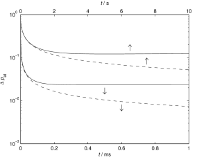
Figure 2: Uncertainty in $p_{\textrm{at}}$ as a function of time with atomic decay included (solid curves) and excluded (dashed curves). The upper and lower curves represent squeezing of the same atomic system in free space and in a cavity, respectively. Note the different time scales. The parameters are (see madsen ): $N_{at}=10^{12}$, $\Phi=10^{14}\textrm{ s}^{-1}$ for $t>0$, $A=2\textrm{ cm}^{2}$, $\tau=3\cdot 10^{-10}\textrm{ s}$, $\Delta=2\pi\cdot 10^{10}\textrm{ Hz}$, $\lambda=852\textrm{ nm}$, $\Gamma=3.1\cdot 10^{7}\textrm{ s}^{-1}$, $d=2.61\cdot 10^{-29}\textrm{ Cm}$, $\kappa=\kappa_{1}=2\pi\cdot 3\cdot 10^{6}\textrm{ Hz}$ (i.e., we observe the reflected light and assume $\kappa_{L}=0$), and $\eta_{d}=1$.

Integrating the Ricatti equation numerically, we obtain the lower curves in Fig. 2, where $\Delta p_{\textrm{at}}\equiv(\textrm{Var}(\hat{p}_{\textrm{at}}))^{1/2}$. For the chosen parameters $\tilde{g}(\tau\ll t\ll\eta(t\gg\tau)^{-1})\tau=2\cdot 10^{-3}$, $\kappa\tau=6\cdot 10^{-3}$, and $\Phi\tau=3\cdot 10^{4}$, and the requirements of a dilute atomic gas, a high finesse cavity, and a strong local oscillator are satisfied. The values $\langle\hat{J}_{x}(0)\rangle/\hbar=5\cdot 10^{11}\gg 1$ and $\langle\hat{a}_{x}(t\gg\tau)\rangle=4.6\cdot 10^{3}\gg 1$ justify the classical treatment of these quantities, and $t=1\textrm{ ms}$ satisfies $t\ll(4\eta_{d}\kappa_{2}\alpha(t\gg\tau)^{2})^{-1}=2.7\cdot 10^{4}\textrm{ s}$ and $t\ll\eta(t\gg\tau)^{-1}=0.13\textrm{ s}$. When atomic decay is included, the uncertainty in $p_{\textrm{at}}$ does not decrease indefinitely, but begins to rise at a certain point if the probing is continued. For the given example, the minimum value of the uncertainty is $(\Delta p_{\textrm{at}})_{\textrm{min}}=0.0233$.

For single pass squeezing madsen

$$\left(\frac{d\textrm{Var}(\hat{p}_{\textrm{at}})}{dt}\right)_{\textrm{sp}}=-2N_{\textrm{at}}\Phi\frac{g^{4}\tau^{2}}{\Delta^{2}}\eta_{d}\textrm{Var}(\hat{p}_{\textrm{at}})^{2}e^{-\eta t}\\ -\frac{1}{3}\eta\textrm{Var}(\hat{p}_{\textrm{at}})+\frac{2}{3}\eta e^{\eta t},$$ (49)

and the result of an integration of this equation is shown in Fig. 2 for comparison. The squeezing is seen to occur on a significantly slower time scale, and we note that $Q=5\cdot 10^{5}$ for the chosen parameters. The attained minimum value of the uncertainty $(\Delta p_{\textrm{at}})_{\textrm{min}}=0.121$ is also significantly higher. This value is in accordance with the value $0.118$ obtained from the approximate relation

$$(\Delta p_{\textrm{at}})_{\textrm{min}}=\left(\frac{\eta\Delta^{2}}{3N_{\textrm{at}}\Phi g^{4}\tau^{2}\eta_{d}}\right)^{1/4}$$ (50)

derived in madsen (we have included an additional factor of $2/3$ to take the factors $1/3$ and $2/3$ in Eq. (38) into account). Since we found in Sec. III that the main effect of the cavity is to increase the squeezing rate by $Q$, and since it follows from (44) that $\eta$ is a factor $4\kappa_{1}/((\kappa+\epsilon)^{2}\tau)$ larger for squeezing in a cavity than for single-pass squeezing, we expect that $(\Delta p_{\textrm{at}})_{\textrm{min}}$ is decreased by a factor $((\kappa+\epsilon)^{2}\tau/(4\kappa_{2}))^{1/4}$ if the atoms are enclosed in a cavity. This leads to the predicted value $(\Delta p_{\textrm{at}})_{\textrm{min}}=0.0230$ for squeezing in a cavity, which is close to the value observed in Fig. 2. Since $(\Delta p_{\textrm{at}})_{\textrm{min}}$ is proportional to $N_{\textrm{at}}^{-1/4}$, we could also regard the squeezing enhancement factor as a multiplicative factor on $N_{\textrm{at}}$, and this opens the way to use the cavity to achieve measurement induced squeezing of a smaller number of atoms. For $N_{\textrm{at}}=10^{12}\cdot(\kappa+\epsilon)^{2}\tau/(4\kappa_{2})=1.4\cdot 10^{9}$ we thus find a minimum uncertainty of 0.121 after a probing time of 7 ms. We note that $\tilde{g}(t)$, $\eta(t)$, and $\epsilon$ are all unchanged if $\Phi$, $N_{\textrm{at}}$, and $A$ are scaled by a common factor, and we thus obtain the same result for $7\cdot 10^{6}$ atoms if $\Phi=5\cdot 10^{11}\textrm{ s}^{-1}$ and $A=10^{-6}\textrm{ m}^{2}$. A further decrease in $\Phi$ would, however, violate the assumption of a classical $x$-polarized field and the approximation below Eq. (42).

V Conclusion

We have considered squeezing of one component of the collective spin of an atomic ensemble achieved by performing homodyne measurements on light, which has interacted with the atoms, and we have found that the squeezing rate can be increased by a factor $Q=16\kappa_{1}\kappa_{2}/(\kappa^{4}\tau^{2})$ by placing the atoms inside an optical cavity. For ensembles containing a large number of atoms initially prepared in a coherent spin state, an efficient Gaussian formalism is applicable, from which we have derived equations for the time evolution of the covariance matrix describing the state of the atomic spin and the cavity field, but we have also demonstrated that analytical results for the state can be obtained even if the state of the atomic spin is not Gaussian. Despite the stochastic nature of the measurements, the variances of the components of the atomic spin and the quadratures of the light field evolve deterministically in the Gaussian approximation, and, in the lossless case, the variance of the squeezed atomic spin component is a monotonically decreasing function of time. According to the Heisenberg uncertainty relation the variance of the conjugate atomic spin variable has to increase, and the uncertainty product only attains the smallest allowed value if all photons, transferred to the mode with polarization orthogonal to the polarization of the probe beam due to the interaction with the atoms, have left the cavity and been detected at the considered time. Allowing the atoms to decay spontaneously, we find that the minimum variance of the squeezed spin component is obtained much faster and is approximately reduced by a factor $((\kappa+\epsilon)^{2}\tau/(4\kappa_{2}))^{1/2}$ compared to the single-pass setup.

References

• (1) L-M Duan, J. I. Cirac, P. Zoller, and E. S. Polzik, Phys. Rev. Lett. 85, 5643 (2000).
• (2) B. Julsgaard, A. Kozhekin, and E. S. Polzik, Nature (London) 413, 400 (2001).
• (3) J. F. Sherson, H. Krauter, R. K. Olsson, B. Julsgaard, K. Hammerer, I. Cirac, and E. S. Polzik, Nature (London) 443, 557 (2006).
• (4) J. F. Sherson and K. Mølmer, Phys. Rev. Lett. 97, 143602 (2006).
• (5) K. Hammerer, K. Mølmer, E. S. Polzik, and J. I. Cirac, Phys. Rev. A 70, 044304 (2004).
• (6) A. Kuzmich, N. P. Bigelow, and L. Mandel, Europhys. Lett. 42, 481 (1998).
• (7) Y. Takahashi, K. Honda, N. Tanaka, K. Toyoda, K. Ishikawa, and T. Yabuzaki, Phys. Rev. A 60, 4974 (1999).
• (8) A. Kuzmich, L. Mandel, and N. P. Bigelow, Phys. Rev. Lett. 85, 1594 (2000).
• (9) L. K. Thomsen, S. Mancini, and H. M. Wiseman, Phys. Rev. A 65, 061801(R) (2002).
• (10) JM Geremia, J. K. Stockton, H. Mabuchi, Science 304, 270 (2004);
• (11) L. B. Madsen and K. Mølmer, Phys. Rev. A 70, 052324 (2004).
• (12) J. Sherson and K. Mølmer, Phys. Rev. A 71, 033813 (2005).
• (13) D. Budker and M. Romalis, Nature Physics 3, 227 (2007).
• (14) H. L. Partner, B. D. Black, and JM Geremia, arXiv:0708.2730.
• (15) A. E. B. Nielsen and K. Mølmer, Phys. Rev. A 76, 033832 (2007).
• (16) A. E. B. Nielsen and K. Mølmer, arXiv:0802.1225.