New Strings for Old Veneziano

Amplitudes IV. Connections

With Spin Chains and Other

Stochastic Systems

                                                                  

Arkady Kholodenko

375 H.L.Hunter Laboratories, Clemson University,

Clemson,  SC 29634-0973, U.S.A.

E-mail: string@clemson.edu

Abstract: In a series of recently published papers we reanalyzed the existing treatments of the Veneziano and Veneziano-like amplitudes and the models associated with these amplitudes. In this work we demonstrate that the already obtained  new partition function for these amplitudes can be exactly mapped into that for the Polychronakos-Frahm (P-F) spin chain model which, in turn, is obtainable from the Richardon-Gaudin (R-G) XXX model. Reshetikhin and Varchenko demonstrated that such a model is obtainable as a leading approximation in their WKB-type analysis of solutions of  the Knizhnik-Zamolodchikov (K-Z) equations. The linear independence of solutions of these equations is controlled by determinants (discovered by Varchenko) whose explicit form up to a constant coincides with the Veneziano (or Veneziano-like) amplitudes. In the simplest case, when K-Z equations are reducible to the Gauss hypergeometric equation, the determinantal conditions coincide with those which were discovered by Kummer in 19-th century. Kummer’s results admit physical interpretation crucial for providing needed justification associating determinantal formula(s) with Veneziano-like amplitudes. General results are illustrated by many examples. These include but are not limited  to only high energy physics since all high energy physics scattering processes can be looked upon from much broader stochastic theory of random fragmentation and coagulation processes  recently undergoing active development in view of its applications in disciplines ranging from ordering in spin glasses and population genetics to computer science, linguistics and economics, etc. In this theory  Veneziano amplitudes play a central (universal) role since they are the Poisson-Dirichlet-type distributions for these processes (analogous to the more familiar Maxwell distribution for gases).

Keywords: Polychronakos and Richardson-Gaudin  spin chains, Knizhnik-Zamolodchikov equations, determinantal formulas, Veneziano amplitudes, random fragmentation-coagulation processes.

Contents

1.Introduction

2.Combinatorics of Veneziano amplitudes and spin chains:

qualitative considerations

3.Connection with the Polychronakos-Frahm (P-F) spin

chain model

4.Connections with WZNW model and XXX s=1/2 Heisenberg

antiferromagnetic spin chain

4.1  General remarks

4.2 Method of generating functions andq-deformed harmonic oscillator

4.3 The limit $q\rightarrow 1^{\pm}$ and emergence of the Stiltjes-Wiegert polynomials

4.4 ASEP, q-deformed harmonic oscillator and spin chains

4.5 Crossover between the XXZ and XXX spin chains: connections

with the KPZ and EW equations and the lattice Liouville model

4.6 ASEP, vicious random walkers and string models

5. Gaudin model as linkage between the WZNW model and K-Z

equations. Recovery of the Veneziano-like amplitudes

5.1 General remarks

5.2 Gaudin magnets, K-Z equation and P-F spin chain

5.3 The Shapovalov form

5.4 Mathematics and physics of the Bethe ansatz equations for XXX

Gaudin model according to works by Richardson. Connections

with the Veneziano model

5.5 Emergence of the Veneziano-like amplitudes as consistency condition

for N=1 solutions of K-Z equations. Recovery of the pion-pion

scattering amplitude

6. Discussion. Unimaginable  ubiquity of the Veneziano-type

amplitudes in Nature

6.1  General remarks

6.2. Random fragmentation and coagulation

processes and the Dirichlet distribution

6.3  The Ewens sampling formula and Veneziano amplitudes

6.4  Stochastic models for second order chemical reaction

kinetics involving Veneziano-like amplitudes

6.4.1Quantum mechanics, hypergeometric functions and the

Poisson-Dirichlet distribution

6.4.2 Hypergeometric functions, Kummer series expansions and

Veneziano-like amplitudes

A. Basics of ASEP

A.1 Equations of motion and spin chains

A.2 Dynamics of ASEP and operator algebra

A.3 Steady -state and q-algebra for the deformed harmonic oscillator

B. Linear independence of solutions of K-Z equation

C. Connections between the gamma and Dirichlet

distributions

D. Some facts from combinatorics of the symmetric group

1 Introduction

Since time when quantum mechanics (QM) was born (in 1925-1926) two seemingly opposite approaches for description of atomic and subatomic physics were proposed respectively by Heisenberg and Schrödinger. Heisenberg’s approach is aimed at providing an affirmative answer to the following question: Is combinatorics of spectra (of obsevables)  provides sufficient  information about microscopic system so that dynamics of such a system can be described in terms of known macroscopic concepts? Schrodinger’s approach is exactly opposite and is aimed at providing an affirmative answer to the following question: Using some plausible mathematical arguments is it possible to find an equation which under some prescribed restrictions will reproduce the spectra of observables? Although it is widely believed that both approaches are equivalent, already Dirac in his lectures on quantum field theory [1] noticed (without much elaboration) that Schrodinger’s description of QM contains a lot of ”dead wood” which can be safely disposed altogether. According to Dirac  ”Heisenberg’s picture of QM is good because Heisenberg’s equations of motion make sense”.

To our knowledge, Dirac’s comments were completely ignored, perhaps, because he had not provided enough evidence making Heisenberg’s description of QM superior to that of Schrodinger’s. In recent papers [2,3] we found examples supporting Dirac’s claims. From the point of view of combinatorics, there is not much difference in description of QM, quantum field theory and string theory. Therefore, in this paper we choose the Heisenberg’s point of view on string theory using results of our recent works in which we re analyzed the existing treatments connecting Veneziano (and Veneziano-like) amplitudes with the respective string-theoretic models. As result, we were able to find new tachyon-free models reproducing Veneziano (and Veneziano-like) amplitudes. In this work the result of our  papers [4-6] which will be called as Part I, Part II and Part III respectively, are  developed further to bring them in correspondence with those proposed by other authors. Without any changes in the already developed formalism, we were able to connect our results with an impressive number of string-theoretic models, including the most recent ones. Nevertheless, below we argue that, although physically plausible, the established connections (in the way they are typically treated in physics literature) are mathematically ill founded. To correct this deficiency, in Section 5 we use some works by mathematicians. Of particular importance for us are the works by Reshetikhin and Varchenko [7]  and by Varchenko summarized in Varchenko’s  MIT lecture notes [8]. These works enabled us to relate Veneziano (and Veneziano-like) amplitudes (e.g. those describing $\pi\pi$ scattering) to Knizhnik-Zamolodchikov (K-Z) equations and, hence, to WZNW models. This is achieved by employing known connections between the WZNW models and spin chains. In the present case, between the K-Z equations and the XXX-type Richardson-Gaudin magnetic chains as described in Section 5. Sections 2-4 contain mathematically less sophisticated results aimed at providing needed physical  motivations and background. For this purpose in section 2 we replaced mathematically sophisticated derivation of the  Veneziano partition function by considerably simpler combinatorial derivation of such function. As a by product of this effort we were able to uncover the connections with spin chains already at this stage of our investigation. To strengthen this connection, in Section 3 we demonstrate that  the obtained Veneziano partition function  coincides with the Polychronakos-Frahm (P-F) partition function for the ferromagnetic spin chain model. Although such  a spin chain was extensively studied in literature, we discuss different paths in Section 4 aimed at establishing links between the P-F spin chain and variety of string-theoretic models, including the most recent ones. This is achieved by mapping  combinatorial and analytical properties  of the P-F spin chains into analogous properties of spin chains used for description of the stochastic process known as asymptotic simple exclusion process (ASEP). To make our presentation self-contained, we provide in Appendix A basic information on ASEP sufficient for understanding the results discussed in the main text. In addition, in the main text we provide some information on Kardar-Parisi-Zhang (KPZ) and Edwards-Wilkinson (EW) equations which are just different well defined macroscopic limits of the microscopic ASEP equations. We do this with purpose of  reproducing variety of string-theoretic models, including the most recent ones. Such a success have not deterred us from looking at other, more rigorous (mathematically) approaches. These are discussed in Sections 5 and, in part, in Section 6. These sections are interrelated and contain the most important results of this paper. While the content of Section 5 was already briefly discussed, the content of Section 6 provides the strongest independent support to the results and conclusions of Section 5. At the same time, this section can be read independently of the rest of the paper since it contains some important facts from  the theory of random fragmentation and coagulation processes [9-11] which is currently in the process of rapid development because of its wide applications ranging from theory of spin glasses and population genetics to computer science, linguistics and economics, etc. In high energy physics this theory was developed for some time by Mekjian, e.g. see [12] and references therein.  Since our Section 6 is not a review, our treatment of topics discussed in it is markedly different from that developed in Mekjian’s papers and is subordinated to the content of Section 5. Specifically, the main result of Section 5 is the deteminantal formula, equation (5.47), which up to a constant coincides with the Veneziano (or Veneziano-like) amplitude. A special case of this formula produces known pion-pion scattering amplitude. In Section 6 we argue that: 1. Veneziano amplitudes play the central role in the theory of random fragmentation and coagulation processes where they are known as the Poisson-Diriclet (P-D) probability distributions. 2.  The discrete spectra of all exactly solvable quantum mechanical (QM) problems can be rederived in terms of some P-D stochastic processes. This is so because all exactly solvable QM problems involve some kind of orthogonal polynomials-all derivable from the Gauss hypergeometric function which admits an interpretation in terms of the P-D process. 3. Since in the simplest case the K-Z equations are reducible to the hypergeometric equations, the processes they describe are also of P-D type. 4. In the case of  Gauss hyprgeometric equation, the determinantal formula (5.47) is reduced to that obtained by Kummer in 19th century. To facilitate understanding  and appreciation of these facts and to demonstrate utility of the obtained results beyond the scope of high energy physics, in Section 6 we discuss some applications of the developed formalism to genetics and chemical kinetics.

2 Combinatorics of Veneziano amplitudes and spin chains: qualitative considerations

In Part I, we noticed that the Veneziano condition for the 4-particle amplitude given by

$$\alpha(s)+\alpha(t)+\alpha(u)=-1,$$ (2.1)

where $\alpha(s)$, $\alpha(t),\alpha(u)$ $\in\mathbf{Z}$, can be rewritten in more mathematically suggestive form. To this purpose, following [13], we need to consider additional homogenous equation of the type

$$\alpha(s)m+\alpha(t)n+\alpha(u)l+k\cdot 1=0$$ (2.2)

with $m,n,l,k$ being some integers. By adding this equation to (2.1) we obtain,

$$\alpha(s)\tilde{m}+\alpha(t)\tilde{n}+\alpha(u)\tilde{l}=\tilde{k}$$ (2.3a)

or, equivalently, as

$$n_{1}+n_{2}+n_{3}=\hat{N},$$ (2.3b)

where all entries by design are nonnegative integers. For the multiparticle case this equation should be replaced by

$$n_{0}+\cdot\cdot\cdot+n_{k}=N$$ (2.4)

so that combinatorially the task lies in finding all nonnegative integer combinations of $n_{0},...,n_{k}$ producing (2.4). It should be noted that such a task makes sense as long as $N$ is assigned. But the actual value of $N$ is not fixed and, hence, can be chosen quite arbitrarily. Equation (2.1) is a simple statement about the energy -momentum conservation. Although the numerical entries in this equation can be changed as we just explained, the actual physical values can be  subsequently re obtained by the appropriate coordinate shift. Such a procedure should be applied to the amplitudes of conformal field theories (CFT)  with some caution  since the periodic ( or antiperiodic, etc.) boundary conditions cause energy and momenta to become a quasi -energy and a quasi momenta (as  it is known from solid state physics).

The arbitrariness of selecting $N$ reflects a kind of gauge freedom. As in other gauge theories, we may try to fix the gauge by using some physical considerations. These include, for example, an observation made in Part I that the 4 particle amplitude is zero if any two entries into (2.1) are the same. This  fact prompts us to arrange the entries in (2.3b) in accordance with their magnitude, i.e. $n_{1}\geq n_{2}\geq n_{3}.$ More generally, we can write: $n_{0}\geq n_{1}\geq\cdot\cdot\cdot\geq n_{k}\geq 1$.

In Section 6 we demonstrate that if the entries in this sequence of inequalities are treated as random nonnegative numbers subject to the constraint (2.4), these constrains are necessary and sufficient for recovery of the probability density for such set of random numbers. This density  is known in mathematics as Dirichlet distribution [9-11,14]. Without normalization, integrals over this distribution coincide with Veneziano amplitudes.

Provided that (2.4) holds, we shall call such a sequence a partition and shall denote it as $\mathit{n\equiv}(n_{0},...,n_{k})$. If $n$ is partition of $N$, then we shall write $n\vdash N$. It is well known [15,16] that there is one- to -one correspondence between the Young diagrams and partitions. We would like to use this fact in order to design a partition function capable of reproducing the Veneziano (and Veneziano-like) amplitudes. Clearly, such a partition function should also make physical sense. Hence, we would like to provide some qualitative arguments aimed at convincing our readers that such a partition function does exist and is physically sensible.

We begin with observation that there is one- to- one correspondence between the Young tableaux and directed random walks. It is useful to recall details of this correspondence now. To this purpose we need to consider a square lattice and to place on it the Young diagram associated with some particular partition.

Let us choose some $\tilde{n}\times\tilde{m}$ rectangle so that the Young diagram occupies the left part of this rectangle. We choose the upper left vertex of the rectangle as the origin of the $xy$ coordinate system whose $y$ axis (South direction) is directed downwards and $x$ axis is directed Eastwards. Then, the South-East boundary of the Young diagram can be interpreted as directed (that is without self intersections) random walk which begins at $(0,-\tilde{m})$ and ends at $(\tilde{n},0).$ Evidently, such a walk completely determines the diagram. The walk can be described by a sequence of 0’s and 1’s. Say, $0$ for the $x-$ step move and 1 for the $y-$ step move. The totality $\mathcal{N}$ of Young diagrams which can be placed into such a rectangle is in one-to-one correspondence with the number of arrangements of 0’s and 1’s whose total number is $\tilde{m}+\tilde{n}$. Recalling the Fermi statistics, the number $\mathcal{N}$ can be easily calculated and is given by $\mathcal{N}=(m+n)!/m!n!$. It can be represented in two equivalent ways

(3)

Let now $p(N;k,m)$ be the number of partitions of $N$ into $\leq k$  nonnegative parts, each not larger than $m$. Consider the generating function of the following type

$$\mathcal{F}(k,m\mid q)=\mathop{\displaystyle\sum}\limits_{N=0}^{S}p(N;k,m)q^{N}$$ (2.6)

where the upper limit $S$ will be determined shortly below. It is shown in Refs.[15,16] that $\mathcal{F}(k,m\mid q)=\left[\begin{array}[]{c}k+m\\ m\end{array}\right]_{q}\equiv\left[\begin{array}[]{c}k+m\\ k\end{array}\right]_{q}$ where, for instance,$\left[\begin{array}[]{c}k+m\\ m\end{array}\right]_{q=1}=\left(\begin{array}[]{c}k+m\\ m\end{array}\right).$ From this result it should be clear that the expression $\left[\begin{array}[]{c}k+m\\ m\end{array}\right]_{q}$ is the $q-$analog of the binomial coefficient $\left(\begin{array}[]{c}k+m\\ m\end{array}\right).$ In literature [15,16] this $q-$ analog is known as the Gaussian coefficient. Explicitly, it is defined as

$$\left[\begin{array}[]{c}a\\ b\end{array}\right]_{q}=\frac{(q^{a}-1)(q^{a-1}-1)\cdot\cdot\cdot(q^{a-b+1}-1)}{(q^{b}-1)(q^{b-1}-1)\cdot\cdot\cdot(q-1)}$$ (2.7)

for some nonegative integers $a$ and $b$. From this definition we anticipate that the sum defining generating function $\mathcal{F}(k,m\mid q)$ in (2.6) should have only finite number of terms. Equation (2.7) allows easy determination of the upper limit $S$ in the sum (2.6). It is given by $km$. This is just the area of the $k\times m$ rectangle. In view of the definition of $p(N;k,m)$, the number $m=N-k$. Using this fact (2.6) can be rewritten as: $\mathcal{F}(N,k\mid q)=\left[\begin{array}[]{c}N\\ k\end{array}\right]_{q}.$This expression happens to be the Poincare^′ polynomial for the Grassmannian $Gr(m,k)$ of the complex vector space C^Nof dimension $N$ as can be seen from page 292 of the book by Bott and Tu, [18]. From this (topological) point of view the numerical coefficients, i.e. $p(N;k,m),$ in the $q$ expansion of (2.6) should be interpreted as Betti numbers of this Grassmannian. They can be determined recursively using the following property of the Gaussian coefficients [4], page 26,

$$\left[\begin{array}[]{c}n+1\\ k+1\end{array}\right]_{q}=\left[\begin{array}[]{c}n\\ k+1\end{array}\right]_{q}+q^{n-k}\left[\begin{array}[]{c}n\\ k\end{array}\right]_{q}$$ (2.8)

and taking into account that $\left[\begin{array}[]{c}n\\ 0\end{array}\right]_{q}=1.$ We refer our readers to Part II for mathematical proof that $\mathcal{F}(N,k\mid q)$ is indeed the Poincare^′ polynomial for the complex Grassmannian. With this fact proven, we notice that, due to relation $m=N-k,$ it is sometimes more convenient  for us to use the parameters $m$ and $k$ rather than $N$ and $k$. With such a replacement we obtain:

$$\mathcal{F}(k,m \mid q)=\left[\begin{array}[]{c}k+m\\ k\end{array}\right]_{q}=\frac{(q^{k+m}-1)(q^{k+m-1}-1)\cdot\cdot\cdot(q^{m+1}-1)}{(q^{k}-1)(q^{k-1}-1)\cdot\cdot\cdot(q-1)}$$ (37)

$$= \mathop{\displaystyle\prod}\limits_{i=1}^{k}\frac{1-q^{m+i}}{1-q^{i}}.\TCItag{2.9}$$ (38)

This result is of central importance. In our work, Part II, considerably more sophisticated mathematical apparatus was used to obtain it (e.g. see equation (6.10) of this reference and arguments leading to it).

In the limit : $q\rightarrow 1$ (2.9) reduces to $\mathcal{N}$ as required. To make connections with results known in physics literature we need to re scale $q^{\prime}s$ in (2.9), e.g. let $q=t^{\frac{1}{i}}.$ Substitution of such an expression back into (2.9) and taking the limit $t\rightarrow 1$ again produces $\mathcal{N}$ in view of (2.5). This time, however, we can accomplish more. By noticing that in (2.4) the actual value of $N$ deliberately is not yet fixed and taking into account that $m=N-k$ we can fix $N$ by fixing $m$. Specifically, we would like to choose $m=1\cdot 2\cdot 3\cdot\cdot\cdot k$ and with such a choice we would like to consider a particular term in the product (2.9), e.g.

$$S(i)=\frac{1-t^{1+\frac{m}{i}}}{1-t}.$$ (2.10)

In view of our ”gauge fixing” the ratio $m/i$ is a positive integer by design. This means that we are having a geometric progression. Indeed, if we rescale $t$ again : $t\rightarrow t^{2},$ we then obtain:

$$S(i)=1+t^{2}+\cdot\cdot\cdot+t^{2\hat{m}}$$ (2.11)

with $\hat{m}=\frac{m}{i}.$ Written in such a form the  above sum is just the Poincare^′ polynomial for the complex projective space CP${}^{\hat{m}}.$ This can be seen by comparing pages 177 and 269 of the book by Bott and Tu [18]. Hence, at least for some $m$’s, the Poincare^′ polynomial for the Grassmannian in just the product of the Poincare^′ polynomials for the complex projective spaces of known dimensionalities. For $m$ just chosen, in the limit $t\rightarrow 1,$ we reobtain back the number $\mathcal{N}$ as required. This physically motivating process of gauge fixing just described can be replaced by more rigorous mathematical arguments. The recursion relation (2.8) introduced earlier indicates that this is possible. The  mathematical details leading to factorization which we just described can be found, for instance, in the Ch-3 of lecture notes by Schwartz [19]. The relevant physics emerges by noticing that the partition function $Z(J)$ for the particle with spin $J$ is given by [20]

$$Z(J) = tr(e^{-\beta H(\sigma)})=e^{cJ}+e^{c(J-1)}+\cdot\cdot\cdot+e^{-cJ}$$ (39)

$$= e^{cJ}(1+e^{-c}+e^{-2c}+\cdot\cdot\cdot+e^{-2cJ}),\TCItag{2.12}$$

where $c$ is known constant. Evidently, up to a constant, $Z(J)\simeq S(i).$ Since mathematically the result (2.12) is the Weyl character formula, this fact brings the classical group theory into our discussion. More importantly, because the partition function for the particle with spin $J$ can be written in the language of N=2 supersymmetric quantum mechanical model, as demonstrated by Stone [20] and others [21], the connection between the supersymmetry and the classical group theory is evident.  It was developed in Part III.

In view of arguments presented above, the Poincare^′ polynomial for the Grassmannian can be interpreted as a partition function for some kind of a spin chain made of  apparently independent spins of various magnitudes. These qualitative arguments we would like to make more mathematically and physically rigorous. The first step towards this goal is made in the next section.

3 Connection with the Polychronakos-Frahm spin chain model

The Polychronakos-Frahm (P-F) spin chain model  was originally proposed by Polychronakos and described in detail in [23]. Frahm [24]  motivated by the results of Polychronakos made additional progress in elucidating the spectrum and thermodynamic properties of this model so that it had become known as the P-F model. Subsequently, many other researchers have contributed to our understanding of this exactly integrable spin chain model. Since this paper is not a review, we shall quote only works on P-F model which are of immediate relevance.

Following [23], we begin with some description of the P-F model. Let $\sigma_{i}^{a}$ ($a=1,2,...,n^{2}-1)$ be $SU(n)$ spin operator of i-th particle and let the operator$\ \sigma_{ij}$ be responsible for a spin exchange between particles $i$ and $j,$ i.e.

$$\sigma_{ij}=\frac{1}{n}+\mathop{\textstyle\sum}\limits_{a}\sigma_{i}^{a}\sigma_{j}^{a}.$$ (3.1)

In terms of these definitions, the Calogero-type model Hamiltonian can be written as [25,26]

$$\mathcal{H}=\frac{1}{2}\mathop{\textstyle\sum}\limits_{i}(p_{i}^{2}+\omega^{2}x_{i}^{2})+\mathop{\textstyle\sum}\limits_{i<j}\frac{l(l-\sigma_{ij})}{\left(x_{i}-x_{j}\right)^{2}},$$ (3.2)

where $l$ is some parameter. The P-F model is obtained from the above model in the limit $l\rightarrow\pm\infty$ . Upon proper rescaling of $\mathcal{H}$ in (3.2), in this limit one obtains

$$\mathcal{H}_{\mathcal{P-F}}=-sign(l)\mathop{\textstyle\sum}\limits_{i<j}\frac{\sigma_{ij}}{\left(x_{i}-x_{j}\right)^{2}},$$ (3.3)

where the coordinate $x_{i}$ minimizes the potential for the rescaled Calogero model, that is

$$\omega^{2}x_{i}=\mathop{\textstyle\sum}\limits_{i<j}\frac{2}{\left(x_{i}-x_{j}\right)^{3}}.$$ (3.4)

It should be noted that $\mathcal{H}_{\mathcal{P-F}}$ is well defined without such a minimization, that is for arbitrary real parameters $x_{i}$. This fact will be further explained in Section 5. In the large $l$ limit the spectrum of $\mathcal{H}$ is decomposable as

$$E=E_{\mathcal{C}}+lE_{\mathcal{P-F}}$$ (3.5)

where $E_{C}$ is the spectrum of the spinless Calogero model while $E_{\mathcal{P-F}}$ is the spectrum of the P-F model. In view of such a decomposition, the partition function for the Hamiltonian $\mathcal{H}$ at temperature $T$ can be written as a product: Z${}_{\mathcal{H}}(T)=$Z${}_{\mathcal{C}}(T)$Z${}_{\mathcal{P-F}}(T/l)$. From here, one formally obtains the result:

$$Z_{\mathcal{P-F}}(T)=\lim_{l\rightarrow\infty}\frac{Z_{\mathcal{H}}(lT)}{Z_{\mathcal{C}}(T)}.$$ (3.6)

It implies that the spectrum of the P-F spin chain can be obtained if both the total and  the Calogero partition functions can be calculated. In [23] Polychronakos argued that $Z_{\mathcal{C}}(T)$ is essentially a partition function of $\mathit{N}$ noninteracting harmonic oscillators. Thus, we obtain

$$Z_{\mathcal{C}}(N;T)=\mathop{\textstyle\prod}\limits_{i=1}^{N}\frac{1}{1-q^{i}},\text{ }q=\exp(-\beta),\beta=\left(k_{B}T\right)^{-1}.$$ (3.7)

Furthermore, the partition function $Z_{\mathcal{H}}(T)$ according to Polychronakos can be obtained using $Z_{\mathcal{C}}(N;T)$ as follows. Consider the grand partition function of the type

$$\Xi=\mathop{\textstyle\sum}\limits_{N=0}^{\infty}Z_{n}(N;T)y^{N}\equiv\left(\mathop{\textstyle\sum}\limits_{L=0}^{\infty}Z_{\mathcal{C}}(L;T)y^{L}\right)^{n}$$ (3.8)

where $n$ is the number of flavors.  Using this definition we obtain

$$Z_{n}(N;T)=\sum_{\Sigma_{i}k_{i}=N}\prod\limits_{i=1}^{n}Z_{\mathcal{C}}(k_{i};T).$$ (3.9)

Next, Polychronakos identifies $Z_{n}(N;T)$ with Z${}_{\mathcal{H}}(T)$. Then, with help of (3.6) the partition function $Z_{\mathcal{P-F}}(T)$ is obtained straightforwardly as

$$Z_{\mathcal{P-F}}(N;T)=\sum_{\Sigma_{i}k_{i}=N}\frac{\mathop{\textstyle\prod}\limits_{i=1}^{N}(1-q^{i})}{\prod\limits_{i=1}^{n}\prod\limits_{r=1}^{k_{i}}(1-q^{r})}.$$ (3.10)

Consider this result for a special case: $n=2$. It is convenient to evaluate the ratio first before calculating the sum. Thus, we obtain:

$$\frac{\mathop{\textstyle\prod}\limits_{i=1}^{N}(1-q^{i})}{\prod\limits_{i=1}^{2}\prod\limits_{r=1}^{k_{i}}(1-q^{r})}=\frac{(1-q)\cdot\cdot\cdot(1-q^{N})}{(1-q)\cdot\cdot\cdot(1-q^{k})(1-q)\cdot\cdot\cdot(1-q^{N-k})}\equiv\mathcal{F}(N,k\mid q).$$ (3.11)

where the Poincare^′ polynomial $\mathcal{F}(N,k\mid q)$ for the Grassmanian of the complex vector space C^N of dimension $N$  was obtained in the previous section. Indeed (3.11) can be trivially brought into the same form as given in our equation (2.9) using the relation $m+k=N$. To bring (2.9) in correspondence with equation (4.1) of Polychronakos [23], we use the second equality (2.9)  in which we make a substitution: $m=N-k.$ After this replacement, (3.10) acquires the following form

$$Z_{\mathcal{P-F}}^{f}(N;T)=\sum\limits_{k=0}^{N}\prod\limits_{i=0}^{k}\frac{1-q^{N-i+1}}{1-q^{i}}$$ (3.12)

coinciding with equation (4.1) by Polychronakos. This equation corresponds to the ferromagnetic version of the P-F spin chain model. To obtain the antiferromagnetic version of the model requires us only to replace $q$ by $q^{-1}$ in (3.12) and to multiply the whole r.h.s. by some known power of $q$. Since this factor will not affect thermodynamics, following Frahm [24], we shall ignore it. As result, we obtain

$$Z_{\mathcal{P-F}}^{af}(N;T)=\sum\limits_{k=0}^{N}q^{\left(N/2-k\right)^{2}}\prod\limits_{i=0}^{k}\frac{1-q^{N-i+1}}{1-q^{i}},$$ (3.13)

in accord with Frahm’s equation (21).  This result is analyzed further in the next section.

4 Connections with WZNW model and XXX  s=1/2  Heisenberg antiferromagnetic  spin chain

4.1 General remarks

To establish these connections we follow work by Hikami [27]. For this purpose, we introduce the notation

$$\left(q\right)_{n}=\prod\limits_{i=1}^{n}(1-q^{i})$$ (4.1)

allowing us to rewrite (3.13) in the equivalent form

$$Z_{\mathcal{P-F}}^{af}(N;T)=\sum\limits_{k=0}^{N}q^{\left(N/2-k\right)^{2}}\prod\limits_{i=0}^{k}\frac{1-q^{N-i+1}}{1-q^{i}}=\sum\limits_{k=0}^{N}q^{\left(N/2-k\right)^{2}}\frac{\left(q\right)_{N}}{\left(q\right)_{k}\left(q\right)_{N-k}}.$$ (4.2)

Consider now the limiting case ($N\rightarrow\infty)$ of the obtained expression.  For this purpose we need to take into account that [andrews1]

$$\lim_{N\rightarrow\infty}\left[\begin{array}[]{c}N\\ k\end{array}\right]_{q}=\frac{1}{\left(q\right)_{k}}.$$ (4.3)

To use this asymptotic result in (4.2) it is convenient to consider separately the cases of $N$ being even and odd. For instance, if $N$ is even, we can write: $N=2m.$ In such a case we can introduce new summation variables: $l=k-m$ and/or $l=m-k.$ Then, in the limit $N\rightarrow\infty$ (that is m$\rightarrow\infty)$ we obtain asymptotically

$$Z_{\mathcal{P-F}}^{af}(\infty;T)=\frac{1}{\left(q\right)_{\infty}}\sum\limits_{i=-\infty}^{\infty}q^{i^{2}}.$$ (4.4a)

in accord with [27]. Analogously, if $N=2m+1$, we obtain instead

$$Z_{\mathcal{P-F}}^{af}(\infty;T)=\frac{1}{\left(q\right)_{\infty}}\sum\limits_{i=-\infty}^{\infty}q^{\left(i+\frac{1}{2}\right)^{2}}.$$ (4.4b)

According to Melzer [28] and Kedem, McCoy and Melzer [29], the obtained partition functions coincide with the Virasoro characters for SU₁(2) WZNW  model describing the conformal limit of the XXX (s=1/2) antiferromagnetic spin chain [30]. Even though equations (4.4a) and (4.4b) provide the final result, they do not reveal their physical content. This task was accomplished in part in the same papers where connection with the excitation spectrum of the XXX antiferromagnetic chain  was made. To avoid repetitions,  below we arrive at these results using different arguments. By doing so many new and unexpected connections  with other  stochastic models will be uncovered.

4.2 Method of generating functions and q-deformed harmonic oscillator

We begin with definitions. In view of (2.9),(3.12) and (4.2), we would like to introduce the Galois number $G_{N}$ via

$$G_{N}=\sum\limits_{k=0}^{N}\left[\begin{array}[]{c}N\\ k\end{array}\right]_{q}.$$ (4.5)

This number can be calculated recursively as it was shown by Goldman and Rota [31] with the result

$$G_{N+1}=2G_{N}+\left(q^{N}-1\right)G_{N-1}.$$ (4.6)

Alternative proof is given by Kac and Cheung [32]. To calculate $G_{N}$ we have to take into account that $G_{0}=1$ and $G_{1}=2.$ These results can be used as a reference when one attempts to calculate the related Rogers-Szego (R-S) polynomial $H_{N}(t)$ defined as [33]

$$H_{N}(t;q):=\sum\limits_{k=0}^{N}\left[\begin{array}[]{c}N\\ k\end{array}\right]_{q}t^{k}$$ (4.7)

so that $H_{N}(1)=G_{N}.$ Using [32] once again, we find that $H_{N}(t)$ obeys the following recursion relation

$$H_{N+1}(t)=(1+t)H_{N}(t)+\left(q^{N}-1\right)tH_{N-1}(t)$$ (4.8)

which for $t=1$ coincides with (4.6) as required. The above recursion relation is supplemented with initial conditions. These are : $H_{0}=1$ and $H_{1}=1+t$.

At this point we would like to remind our readers that for $t=1$ according to (3.12) we obtain: $Z_{\mathcal{P-F}}^{f}(N;T)=G_{N}$. Hence, by calculating $H_{N}(t)$ we shall obtain the partition function for the P-F chain.

To proceed with such calculations, we follow [34]. In particular, consider first an auxiliary recursion relation for the Hermite polynomials:

$$H_{n+1}(x)=2xH_{n}(x)-2nH_{n-1}(x)$$ (4.9a)

supplemented by the differential relation

$$\frac{d}{dx}H_{n}(x)=2nH_{n-1}(x)$$ (4.9b)

which, in view of (4.9a), can be conveniently rewritten as

$$H_{n+1}(x)=(2x-\frac{d}{dx})H_{n}(x).$$ (4.9c)

This observation prompts us to introduce the raising operator $R=2x-\dfrac{d}{dx}$ so that we obtain:

$$R^{n}H_{0}(x)=H_{n}(x).$$ (4.10)

The lowering operator can be now easily obtained again using (4.9). We get

$$\frac{1}{2}\frac{d}{dx}H_{n}(x)\equiv LH_{n}(x)=nH_{n-1}(x)$$ (4.11)

so that $[L,R]=1$ as required.  Based on this,the number operator $N$ can be obtained as $N=RL$ so that $NH_{n}(x)=nH_{n}(x)$ or, explicitly, using provided definitions, we obtain

$$(\frac{d^{2}}{dx^{2}}-2x\frac{d}{dx}+2n)H_{n}(x)=0.$$ (4.12)

Evidently, we can write: $R\mid n>=\mid n+1>,$ $L\mid n>=\mid n-1>$ and , $<m\mid n>=n!\delta_{mn}$ as usual.

We would like now to transfer all these results to our main object of interest- the recursion relation (4.8). To this purpose, we introduce the difference operator $\Delta$ via

$$\Delta H_{N}(t):=H_{N}(t)-H_{N}(qt).$$ (4.13)

Using definition (4.7) we obtain now

$$\Delta H_{N}(t)=(1-q^{N})tH_{N-1}(t)$$ (4.14)

where we took into account that

$$\left[\begin{array}[]{c}N\\ k\end{array}\right]_{q}=\left[\begin{array}[]{c}N\\ N-k\end{array}\right]_{q}.$$ (4.16)

Using this result in (4.8) we obtain at once

$$H_{N+1}(t)=[(1+t)-\Delta]H_{N}(t).$$ (4.17)

This, again, can be looked upon as a definition of a raising operator so that we can formally rewrite (4.17) as

$$\mathcal{R}H_{N}(t)=H_{N+1}(t).$$ (4.18)

The lowering operator can be defined now as

$$\mathcal{L}:=\frac{1}{x}\Delta$$ (4.19)

so that

$$\mathcal{L}H_{N}(t)=(1-q^{N})H_{N-1}(t).$$ (4.20)

The action of the number operator $\mathcal{N}=\mathcal{RL}$ is  now straightforward, i.e.

$$\mathcal{N}H_{N}(t)=(1-q^{N})H_{N}(t).$$ (4.21)

Following Kac and Cheung [32] we introduce the $q-$derivative via

$$D_{q}f(x):=\frac{f(qx)-f(x)}{x(q-1)}.$$ (4.22)

By combining this result with (4.13) we obtain,

$$D_{q}f(x)=\frac{\Delta f(x)}{x(1-q)}.$$ (4.23)

This allows us to rewrite the raising and lowering operators in terms of $q-$derivatives. Specifically, we obtain:

$$\mathcal{\tilde{R}}\text{ :}\mathcal{=}(1+t)-(1-q)tD_{q}$$ (4.24)

and

$$\mathcal{\tilde{L}}:=D_{q}.$$ (4.25)

While for the raising operator rewritten in such a way equation (4.18) still holds, for the lowering operator $\mathcal{\tilde{L}}$ we now obtain:

$$\mathcal{\tilde{L}}H_{N}(t)=\frac{1-q^{N}}{1-q}H_{N-1}(t)\equiv[N]H_{N-1}(t).$$ (4.26)

The number operator $\mathcal{N}_{q}$ is acting in this case as

$$\mathcal{N}_{q}H_{N}(t)=[N]H_{N}(t).$$ (4.27)

We would like to connect these results with those available in literature on $q-$deformed harmonic oscillator. Following Chaichan et al [35], we notice that the undeformed oscillator algebra is given in terms of the following commutation relations

$$aa^{+}-a^{+}a=1$$ (4.28a)

$$[N,a]=-a$$ (4.28b)

and

$$[N,a^{+}]=a^{+}.$$ (4.28c)

In these relations it is not assumed a priori that $N=a^{+}a$ and, therefore, this algebra is formally different from the traditionally used $[a,a^{+}]=1$ for the harmonic oscillator. This observation allows us to introduce the central element $Z=N-a^{+}a$ which is zero for the standard oscillator algebra. The deformed oscillator algebra can be obtained now using equations (4.28) in which one should replace (4.28a) by [floreanni&vinet]

$$aa^{+}-qa^{+}a=1.$$ (4.28d)

Consider now the combination $K:=$ $\mathcal{LR}$-$q\mathcal{N}$ acting on $H_{N}$ using previously introduced definitions. A simple calculation produces an operator identity: $\mathcal{LR}-q\mathcal{N=}1$ so that we can formally make a provisional identification : $\mathcal{L\rightarrow}a$ and $\mathcal{R\rightarrow}a^{+}.$ To proceed, we need to demonstrate that with such an identification equations (4.28 b,c) hold as well. For this to happen, we should  properly normalize our wave function in accord with known procedure for the harmonic oscillator where we have to use $\mid n>=\dfrac{1}{\sqrt{n!}}\left(a^{+}\right)^{n}\mid 0>$. In the present case, we have to use $\mid N>=\dfrac{1}{\sqrt{[N]!}}\left(\mathcal{R}\right)^{n}\mid 0>$ as the basis wavefunction while making an identification: $\mid 0>=$ $H_{0}(t).$ The eigenvalue equation (4.27), when written explicitly, acquires the following form:

$$[tD_{q}^{2}-\frac{1+t}{1-q}D_{q}+\frac{[N]}{1-q}]H_{N}(t)=0.$$ (4.29)

4.3 The limit $q\rightarrow 1^{\pm}$ and emergence of the Stieltjes-Wigert polynomials

Obtained results need further refinements for the following reasons. Although the recursion relations (4.8), (4.9) look similar, in the limit $q\rightarrow 1^{\pm}$ (4.8) is not transformed into (4.9). Accordingly, (4.29) is not converted into equation for the Hermite polynomials known for harmonic oscillator.  Fortunately, the situation can be repaired in view of recent paper by Karabulut [37] who spotted and corrected some error in the influential earlier paper by Macfarlane [39]. Following [38] we define the translation operator $T(s)$ as $T(s):=e^{s\frac{\partial}{\partial x}}$. Using this definition, the creation $a^{{\dagger}}$ and annihilation $a$ operators are defined as follows

$$a^{{\dagger}}=\frac{1}{\sqrt{1-q}}[q^{x+\frac{1}{4}}-T^{\frac{-1}{2}}(s)]T^{\frac{-1}{2}}(s)$$ (4.30a)

where $T^{\frac{1}{2}}(s)=e^{\frac{s}{2}\frac{\partial}{\partial x}}$ and, accordingly,

$$a=\frac{1}{\sqrt{1-q}}T^{\frac{1}{2}}(s)[q^{x+\frac{1}{4}}-T^{\frac{1}{2}}(s)].$$ (4.30b)

Under such conditions, the inner product is defined in the standard way, that is

$$(f,g)=\int\limits_{-\infty}^{\infty}f^{\ast}(x)g(x)dx$$ (4.31)

so that $(q^{x})^{{\dagger}}=q^{x}$ and $(\partial/\partial x)^{{\dagger}}=-(\partial/\partial x)$ thus making the operator $a^{{\dagger}}$ to be a conjugate of $a$ in a usual way.The creation-annihilation operators just defined satisfy commutation relation (4.28 d). At the same time, the combination $a^{{\dagger}}a\$ while acting on the wave functions $\Psi_{n\text{ }}$ (to be defined below)  produces equation similar to (4.27), that is

$$a^{{\dagger}}a\Psi_{n\text{ }}=[n]\Psi_{n\text{ }}\equiv\lambda_{n}\Psi_{n\text{ }}.$$ (4.32)

Furthermore, it can be shown that

$$a\Psi_{n\text{ }}=\sqrt{\lambda_{n}}\Psi_{n-1\text{ }}\text{ \ \ and \ }a^{{\dagger}}\Psi_{n\text{ }}=\sqrt{\lambda_{n+1}}\Psi_{n+1\text{ }}$$ (4.33)

in accord with previously obtained results. Next, we would like to obtain the wave function $\Psi_{n\text{ }}$ explicitly. To this purpose we start with the ground state $a\Psi_{0\text{ }}=0$ and use (4.30b) to get (for s=1/2) the following result

$$\Psi_{0\text{ }}(x+\frac{1}{2})=q^{\frac{1}{4}+x}\Psi_{0\text{ }}(x).$$ (4.34)

Let $w(x)$ be some yet unknown function. Then, it is appropriate to look for solution of (4.34) in the form

$$\Psi_{0\text{ }}(x)=const\text{ }\cdot w(x)q^{x^{2}},$$ (4.35a)

provided that the function $w(x)$ is periodic:  $w(x)=w(x+1/2).$ The normalized ground state function acquires then the following look

$$\Psi_{0\text{ }}(x)=\alpha_{w}w(x)q^{x^{2}},$$ (4.35b)

where the constant $\alpha_{w}$ is given by

$$\alpha_{w}=\left(\int\limits_{-\infty}^{\infty}dx\left|q^{x^{2}}w(x)\right|^{2}\right)^{-\frac{1}{2}}.$$ (4.35c)

Using this result,  $\Psi_{n\text{ }}$ can be constructed in a standard way through use of the raising operators. There is, however, a faster way to obtain the desired result.  To this purpose, in view of (4.35b), suppose that $\Psi_{n\text{ }}(x)$ can be decomposed as follows

$$\Psi_{n\text{ }}(x)=\frac{\alpha_{w}w(x)}{\sqrt{(q,q)_{n}}}\sum\limits_{k=0}^{\infty}C_{k}^{n}(q)(-1)^{k}q^{\left(n-k\right)/2}q^{(x-k)^{2}}$$ (4.36)

where $(q,q)_{n}=(1-q)(1-q^{2})\cdot\cdot\cdot(1-q^{n})$ and $C_{k}^{n}(q)$ is to be determined as follows. By applying the operator  $a^{{\dagger}}/$ $\sqrt{\lambda_{n+1}}$ to (4.36) and taking into account that  $T^{-\frac{1}{2}}$ $w(x)=w(x-1/2)=w(x)$ (in  view of the periodicity of $w(x)$) we end up with the recursion relation for $C_{k}^{n}(q)$:

$$C_{k}^{n+1}(q)=q^{k}C_{k}^{n}(q)+C_{k-1}^{n}(q).$$ (4.37)

This relation should be compared with that given by (2.8). Andrews [33], page 35, demonstrated that (2.8) and (4.37) are equivalent. Hence, we obtain:

$$C_{k}^{n}(q)=\left[\begin{array}[]{c}n\\ k\end{array}\right]_{q}.$$ (4.38)

This implies that, indeed, up to a constant, the obtained wavefunction should be related to the Rogers-Szego polynomial. This relation is nontrivial however. We would like to discuss it in some detail now.

Following [37,39], let $q=e^{-c^{2}},$ where $c$ is some nonegative number. Introduce the distributed Gaussian polynomials via

$$\Phi_{n}(x)=\sum\limits_{k=0}^{\infty}C_{k}^{n}(q)(-1)^{k}q^{-k/2}q^{(x-k)^{2}}.$$ (4.39)

These polynomials satisfy the following orthogonality relation:

$$\int\limits_{-\infty}^{\infty}\Phi_{n}(x)\Phi_{m}(x)dx=\left\|\Phi_{n}(x)\right\|^{2}\delta_{mn}$$ (4.40)

with

$$\left\|\Phi_{n}(x)\right\|=\left(\frac{\pi}{2c^{2}}\right)^{\frac{1}{4}}q^{-\frac{n}{2}}\sqrt{(q,q)_{n}}.$$ (4.41)

This result calls for change in normalization of $\Phi_{n}(x),$ i.e$.,\phi_{n}(x)=\frac{\Phi_{n}(x)}{\left\|\Phi_{n}(x)\right\|}.$ Under such conditions $\phi_{n}(x)$ coincides with $\Psi_{n\text{ }}(x),$ provided that $w(x)=1.$ Introduce new variable: $u=q^{-2x},$ and consider a shift: $\Phi_{n}(x)\rightarrow\Phi_{n}(x-s).$ Using (4.39), we can write

$$\Phi_{n}(x-s)=u^{s}\exp\{-\left(\ln u\right)^{2}/(-4\ln q)\}P_{n}(u;s)$$ (4.42a)

where

$$P_{n}(u;s)=\sum\limits_{k=0}^{\infty}C_{k}^{n}(q)(-1)^{k}q^{-k/2}q^{(s+k)^{2}}u^{k}.$$ (4.42b)

The orthogonality relation (4.40) is converted then into

$$\int\limits_{0}^{\infty}duu^{2s-1}\exp\{-\left(\ln u\right)^{2}/(-4\ln q)\}P_{n}(u;s)P_{m}(u;s)=\delta_{mn}.$$ (4.43)

In view of (4.43) consider now a special case: $s=1/2$. Then, the weight function is known as ${lognormal}$ distribution and polynomials $P_{n}(u;1/2)$  (up to a constant ) are known as Stieltjes-Wigert (S-W) polynomials. Their physical relevance will be discussed below in Subsection 4.6. In the meantime, we introduce the Fourier transform of $f(x)$ in the usual way as

$$\int\limits_{-\infty}^{\infty}dx\exp(2\pi i\theta x)f(x)=f(\theta)$$ (4.44)

Then, the Parseval relation implies:

$$\int\limits_{-\infty}^{\infty}\Phi_{n}(x)\Phi_{m}(x)dx=\int\limits_{-\infty}^{\infty}\Phi_{n}(\theta)\Phi_{m}(\theta)dx=\left\|\Phi_{n}(x)\right\|^{2}\delta_{mn},$$ (4.45a)

causing

$$\Phi_{n}(\theta)=\left(\frac{\pi}{c^{2}}\right)^{\frac{1}{4}}\exp(-\left(\pi/c\right)\theta^{2})\sum\limits_{k=0}^{\infty}C_{k}^{n}(q)(-q^{-\frac{1}{2}}e^{2\pi i\theta})^{k}.$$ (4.45b)

Comparison between these results and (4.7) produces

$$\int\limits_{-\infty}^{\infty}H_{n}(-q^{-\frac{1}{2}}e^{-2\pi i\theta};q)H_{m}(-q^{-\frac{1}{2}}e^{-2\pi i\theta};q)\exp(-2\left(\pi/c\right)\theta^{2})=\left(\frac{c}{2\pi}\right)^{\frac{1}{2}}q^{-n}(q,q)_{n}\delta_{mn}$$ (4.46a)

which can be alternatively rewritten as

$$\int\limits_{0}^{1}H_{n}(-q^{-\frac{1}{2}}e^{-2\pi i\theta})H_{m}(-q^{-\frac{1}{2}}e^{-2\pi i\theta})\vartheta_{3}(2\pi\theta;q)d\theta=q^{-n}(q,q)_{n}\delta_{mn}$$ (4.46b)

with $\vartheta_{3}(\theta,q)=\sum\limits_{n=-\infty}^{\infty}q^{n^{2}/2}e^{in\theta}$ . That is $\vartheta_{3\text{ \ }}$is one of the Jacobi’s theta functions. In order to use the obtained results, it is useful to compare them against those, known in literature already, e.g. see [40]. Equation (4.46a) is in agreement with (5) of [40] if we make identifications: $\kappa=\pi$ and $c=\sqrt{2}\kappa,$ where $\kappa$ is the parameter introduced in this reference. With help of such an identification we can proceed with comparison. For this purpose, following 40] we introduce yet another generating function

$$S_{n}(t;q):=\sum\limits_{k=0}^{n}\left[\begin{array}[]{c}n\\ k\end{array}\right]_{q}q^{k^{2}}t^{k}$$ (4.47)

so that the S-W polynomials can be written now as [41], page 197,

$$\mathcal{\tilde{S}}_{n}(t;q)=(-1)^{n}q^{\frac{n}{2}}(\sqrt{(q,q)_{n}})^{-1}P_{n}(t;\frac{1}{2})\equiv(-1)^{n}q^{\frac{2n+1}{{}}}(\sqrt{(q,q)_{n}})^{-1}S_{n}(-q^{\frac{1}{2}}t;q),$$ (4.48)

provided that $0<q<1.$ Comparison between generating functions (4.7) and (4.47) allows us to write as well

$$S_{n}(t;q^{-1})=H_{n}(tq^{-n};q),\text{ or, equivalently, }H_{n}(t;q^{-1})=S_{n}(q^{-n}t;q)$$ (4.49)

Using this result we can rewrite the recursion relation (4.8) for $H_{n}(t;q)$ in terms of the recursion relation for $S_{n}(t;q)$ if needed and then to repeat all the arguments with creation and annihilation operators, etc. For the sake of space, we leave this option as an exercise for our readers. Instead, to finish our discussion we would like to show how the obtained polynomials reduce to the usual Hermite polynomials in the limit $q\rightarrow 1^{-}.$ For this purpose we would like to demonstrate that the recursion relation (4.8) is actually the recursion relation for the continuous $q-$Hermite polynomials [42,43]. This means that we have to demonstrate that under some conditions (to be specified) the recursion (4.8) is equivalent to

$$2xH_{n}(x\mid q)=H_{n+1}(x\mid q)+(1-q^{n})H_{n-1}(x\mid q).$$ (4.50)

known for q-Hermite polynomials. To demonstrate the equivalence we assume that $x=\cos\theta$ in (4.50) and then, let $z=e^{i\theta}.$ Furthermore, we assume that

$$H_{n}(x\mid q)=z^{n}H_{n}(z^{-2};q),$$ (4.51)

allowing us to obtain,

$$(z+z^{-1})z^{n}H_{n}=z^{n+1}H_{n+1}+(1-q^{n})z^{n-1}H_{n-1}.$$ (4.52)

Finally, we set z${}^{-1}=\sqrt{t}$ which brings us back to (4.8). This time, however, we can use results known in literature for $q-$Hermite polynomials [41-43] in order to obtain at once

$$\lim_{q\rightarrow 1^{-}}\frac{H_{n}(x\sqrt{\frac{1-q}{2}}\mid q)}{\sqrt{\frac{1-q}{2}}}=H_{n}(x),$$ (4.53)

where $H_{n}(x)$ are the standard Hermitian polynomials. In view of (4.48), (4.49), not surprisingly, the S-W polynomials are also reducible to $H_{n}(x)$. Details can be found in the same references.

4.4 ASEP, q-deformed harmonic oscillator and spin chains

In this subsection we would like to connect the results obtained thus far with the XXX and XXZ spin chains. Although a connection  with XXX  spin chain was established already at the beginning of this section, we would like to arrive at the same conclusions using alternative (physically inspired) arguments and methods. To understand the logic of our arguments we encourage our readers to read Appendix A at this point. In it we provide a self contained summary of results related to the asymmetric simple exclusion process (ASEP), especially emphasizing its connection with static and dynamic properties of XXX and XXZ spin chains.

ASEP was discussed in high energy physics literature, e.g. see [44], in connection with random matrix ensembles. To avoid repeats, we would like to use the results of Appendix A  in order to consider the steady-state regime only. To be in  accord with literature on ASEP, we would like to complicate matters by  imposing some nontrivial boundary conditions.

In the steady -state regime equation (A.12) of Appendix A acquires the form : $SC=\Lambda$. Explicitly,

$$SC=p_{L\text{ }}ED-p_{R}DE.$$ (4.54)

In the steady-state regime, the operator $S$ becomes an arbitrary c-number [45]. In view of this, following Sasamoto [46] we rewrite (4.54) as

$$p_{R}DE-p_{L}ED=\zeta\left(D+E\right).$$ (4.55)

Such operator equation should be supplemented by the boundary conditions which are chosen to be as

$$\alpha<W\mid E=\zeta<W\mid\text{ and }\beta D\mid V>=\zeta\mid V>.$$ (4.56)

The normalized steady-state probability for some configuration $\mathcal{C}$ can be written  now as

$$P(\mathcal{C})=\frac{<W\mid X_{1}X_{2}\cdot\cdot\cdot X_{N}\mid V>}{<W\mid C^{N}\mid V>}$$ (4.57)

with  the operator $X_{i}$ being either $D$ or $E$ depending on wether the $i-$th site is occupied or empty. To calculate $P(\mathcal{C})$ we need to determine $\zeta$ while assuming parameters $\alpha$ and $\beta$ to be assigned. We demonstrate in Appendix A that it is possible to equate $\zeta$ to one  so that, in agreement with [47], we obtain the following representation of $D$ and $E$ operators:

$$D=\frac{1}{1-q}+\frac{1}{\sqrt{1-q}}a,\ \text{\ }E=\frac{1}{1-q}+\frac{1}{\sqrt{1-q}}a^{+}$$

converting equation (4.54) into (4.28d). In view of this mapping into $q-$deformed oscillator algebra, we can expand both vectors $\mid V>$ and $<W\mid$ into a Fourier series, e.g. $\mid V>=\sum\nolimits_{m}\Omega_{m}(V)\mid m>$ where, using (4.33), we put $\mid m>=\Psi_{m}.$ By combining equations (4.33) and (4.56) and results of Appendix A we obtain the following recurrence equation for $\Omega_{n}:$

$$\Omega_{n}(V)(\frac{1-q}{\beta}-1)=\Omega_{n+1}(V)\sqrt{1-q^{n+1}}.$$ (4.58)

Following [47] we assume that $<0\mid V>=1.$ Then, the above  recurrence produces

$$\Omega_{n}(V)=\frac{v^{n}}{\sqrt{(q,q)_{n}}},$$

with  parameter $v=\frac{1-q}{\beta}-1.$ Analogously, we obtain:

$$\Omega_{n}(W)=\frac{w^{n}}{\sqrt{(q,q)_{n}}},$$

with $w=\frac{1-q}{\alpha}-1.$ Obtained results exhibit apparently singular behavior for $q\rightarrow 1^{-}.$ These singularities are only apparent since they cancel out when one computes quantities of physical interest discussed in both [48] and [49]. As results of Appendix A indicate, such a crossover is also nontrivial physically since it involves careful treatment of the transition from XXZ to XXX antiferromagnetic spin chains. Hence, the results obtained thus far enable us to connect the partition function (4.2) (or (4.7)) with either XXX or XXZ spin chains but are not yet sufficient for making an unambiguous choice between these two models. This task is accomplished in the rest of this section.

4.5 Crossover between the XXZ and XXX spin chains: connections with the KPZ and EW equations and the lattice Liouville model

Following Derrida and Malick [49], we notice that ASEP is the lattice version of the famous Kradar-Parisi-Zhang  (KPZ) equation [50]. The transition $q\rightarrow 1^{-}$ corresponds to transition (in the sense of renormalization group analysis) from the regime of ballistic deposition whose growth is described by the KPZ  equation to another regime described by the Edwards-Wilkinson (EW)  equation. In the context of ASEP (that is microscopically) such a transition is discussed in detail in [51]. Alternative treatment is given in [49].   The task of obtaining the KPZ or EW equations from those describing the ASEP is nontrivial and was accomplished only very recently [oliveiraetal, Lazarides]. It is essential for us that in doing so the rules of constructing the restricted solid-on -solid (RSOS) models were invoked. From the work by Huse [54] it is known that such models can be found in four thermodynamic regimes.The crossover from the regime III to regime IV is described by the critical exponents of Friedan, Qui and Shenker unitary CFT series [55]. The crossover from regime III to regime IV happens to be relevant to crossover from the KPZ to EW regime as we would like to explain now.

As results of  Appendix A indicate, the truly asymmetric  simple exclusion process is associated with the XXZ model at the microscopic level and with the KPZ equation/model at the macroscopic level. Accordingly, the symmetric exclusion process is associated with the XXX model at the microscopic level and with the EW equation/model  at the macroscopic level. At the level of Bethe ansatz for open XXZ chain with boundaries full details of the crossover from the KPZ to EW regime were exhaustively worked out only recently [56]. For the purposes of this work it is important to notice that for certain values of parameters the Hamiltonian of  open XXZ spin chain model  with boundaries can be brought  to the following canonical form

$$H_{XXZ}=\frac{1}{2}[\sum\limits_{j=1}^{N-1}(\sigma_{j}^{x}\sigma_{j+1}^{x}+\sigma_{j}^{y}\sigma_{j+1}^{y}+\frac{1}{2}(q+q^{-1})\sigma_{j}^{z}\sigma_{j+1}^{z})+\frac{1}{2}(q-q^{-1})(\sigma_{1}^{z}-\sigma_{N}^{z})].$$ (4.59)

In the case of ASEP we have $q=\sqrt{p_{R}/p_{L}}$ so that for physical reasons parameter $q$ is not complex. However, mathematically, we can allow for $q$  to be complex. In particular, following Pasquer and Saleur [57] we can let $q=e^{i\gamma}$ with $\gamma=\dfrac{\pi}{\mu+1}.$ For such values of $q$ use of finite scaling analysis applied to the spectrum of the above defined Hamiltonian produces  the central charge

$$c=1-\frac{6}{\mu(\mu+1)}\text{ , }\mu=2,3,....$$ (4.60)

of the unitary CFT  series. Furthermore, if $e_{i}$ is the generator of the Temperley-Lieb algebra, then $H_{XXZ}$ can be rewritten as [58]

$$H_{XXZ}=-\sum\limits_{j=1}^{N-1}[e_{i}-\frac{1}{4}(q+q^{-1})].$$ (4.61)

This fact allows us to make immediate connections with quantum groups and theory of knots and links. Below, in Section 5 we shall use different arguments to arrive at similar conclusions. The results just described allow us to connect the CFT and  exactly integrable  lattice models. If this is the case, one can pose the following question: given the connection we just described, can we write down explicitly the corresponding path integral string-theoretic models reproducing results of exactly integrable lattice models at and away from criticality? Before providing  the answer in the following subsection, we would like to conclude this subsection with a partial answer. In particular, we would like to mention the work by Faddeev and Tirkkonen [59] connecting the lattice Liouville model with the spin 1/2 XXZ chain. Based on this result, it should be clear that in the region  $c\leq 1$ it is indeed possible by using combinatorial analysis described above to make a link between the continuum and  the discrete Liouville theories. It can be made in such a way that, at least at crtiticality, the results of exactly integrable 2 dimensional models are in agreement with those which are obtainable field- theoretically. The domain $c>1$ is physically meaningless because the models (other than string-theoretic) we discussed in this section loose their physical meaning in this region. This conclusion  will be further reinforced in the next subsection.

4.6 ASEP, vicious random walkers and string models

We have discussed at length the role of vicious random walkers in derivation of the Kontsevich-Witten (K-W) model in our previous work [60]. Forrester [61] noticed that the random turns vicious walkers model is just a special case of ASEP. Further details on connections between the ASEP, vicious walkers, KPZ and random matrix theory can be found in the paper by Sasamoto [62].  In the paper by Mukhi [63] it is emphasized that while the K-W model is the matrix model representing $c<1$ bosonic string,  the Penner matrix model with imaginary coupling constant is representing $c=1$  Euclidean string on the cylinder of  (self-dual) radius $R=1$ Furthermore, Ghoshal and Vafa [65] have demonstrated that $c=1,R=1$ string is dual to the topological string on a conifold singularity. We shall  briefly discuss this connection below. Before doing so,  it is instructive to discuss the crossover from $c=1$ to $c<1$ string models in terms of vicious walkers. To do so we shall use some results from our work on K-W model and from the paper by Forrester [61].

Thus, we would like to consider planar lattice where at the beginning we place only one directed path P: from $(a,1)$ to $(b,N)$. The information about this path can be encoded into multiset $Hor_{y}(P)$ of y-coordinates of the horizontal steps of P. Let now

$$w(P)=\prod\limits_{i=Hor_{y}(P)}x_{i}.$$ (4.62)

Using these definitions, the extension of these results to an assembly of directed random vicious walkers is given as a product: $W(\hat{P})\equiv w(P_{1})\cdot\cdot\cdot w(P_{k}).$ Finally, the generating function for an assembly of such walkers is given by

$$h_{b-a}(x_{1},...,x_{N})=\sum\limits_{\hat{P}}W(\hat{P}),$$ (4.63)

where $W(\hat{P})$ is made of monomials of the type $x_{1}^{m_{1}}x_{2}^{m_{2}}\cdot\cdot\cdot x_{N}^{m_{N}}$ provided that $m_{1}+\cdot\cdot\cdot+m_{N}=b-a.$ The following theorem [ , ] is of central importance for calculation of such defined generating function.

Given integers $0<a_{1}<\cdot\cdot\cdot<a_{k\text{ \ }}$and $0<b_{1}<\cdot\cdot\cdot<b_{k}$ , let M_i,j be the $k\times k$ matrix M${}_{i,j}=h_{b_{j}-a_{i}}(x_{1},...,x_{N})$ then,

$$\det\mathbf{M}=\sum\limits_{\hat{P}}W(\hat{P})$$ (4.64)

where the sum is taken over all sequences ($P_{1},...,P_{k})\equiv\hat{P}$ of nonintersecting lattice paths $P_{i}:(a_{i},1)\rightarrow(b_{i},N),i=1-k.$

Let now $a_{i}=i$ and $b_{j}=\lambda_{i}+j$ so that $1\leq i,j\leq k$ with $\lambda$ being a partition of $N$ with $k$ parts then, $\det\mathbf{M}=s_{\lambda}(x_{1},...,x_{N}),$ where $s_{\lambda}(\mathbf{x})$ is the Schur polynomial. In our work [60 ] we demonstrated that in the limit $N\rightarrow\infty$ such defined Schur polynomial coincides with the partition(generating) function for the Kontsevich model.  Many additional useful results related to Schur functions are discussed in our recent paper [2].

To get results by Forrester requires us to apply some additional efforts. These are worth discussing. Unlike the K-W case, this time, we need to discuss  the continuous random walks in the plane. Let $x$-coordinate represent ”space” while $y$-coordinate- ”time”. If initially ($t=0$) we had $k$-walkers in the positions $-L$ $<x_{1}<x_{2}<\cdot\cdot\cdot<x_{k\text{ }}<L,$ the same order should persist $\forall$ $t>0$. At each tick of the clock each walker is moving either to the right or to the left with equal probability $p$ (that is we are in the regime appropriate for the XXX spin chain in the ASEP terminology). As before, let x${}_{0}=(x_{1,0},...,x_{k,0})$ be the initial configuration of $k-$walkers and x${}_{f}=(x_{1,f},...,x_{k,f})$ be  the final configuration at time $t$. To calculate the total number of walks starting at $t=0$ at x₀ and ending at time $t$ at x_f we need to know the probability distribution $W_{k}(\mathbf{x}_{0}\rightarrow\mathbf{x}_{f};t)$ that the walkers proceed without bumping into each other. Should these random walks be totally uncorrelated, we would obtain for the probability distribution the standard Gaussian result:

$$W_{k}^{0}(\mathbf{x}_{0}\rightarrow\mathbf{x}_{f};t)=\frac{\exp\{-(\mathbf{x}_{f}-\mathbf{x}_{0})^{2}/2Dt\}}{\left(2\pi Dt\right)^{k/2}}.$$ (4.65)

In the present case the walks are restricted (correlated) so that the probability should be modified. This modification can be found in the work by Fisher and Huse [66]. These authors obtain

$$W_{k}(\mathbf{x}_{0}\rightarrow\mathbf{x}_{f};t)=U_{k}(\mathbf{x}_{0},\mathbf{x}_{f};t)\frac{\exp\{-(\mathbf{x}_{f}^{2}+\mathbf{x}_{0}^{2})/2Dt\}}{\left(2\pi Dt\right)^{k/2}}$$ (4.66)

with

$$U_{k}(\mathbf{x}_{0},\mathbf{x}_{f};t)=\sum\limits_{g\in S_{k}}\varepsilon(g)\exp[\frac{(\mathbf{x}_{f}\cdot g\mathbf{x}_{0})}{Dt}].$$ (4.67)

In this expression $\varepsilon(g)=\pm 1,$ and the index $g$ runs over all members of the symmetric group $S_{k}$. Mathematically, following Gaudin [67], this problem can be looked upon as a problem of a random walk inside the $k-$dimensional kaleidoscope (Weyl cone) usually complicated by imposition of some boundary conditions at the walls of the cone. Connection of such random walk problem with random matrices was discussed by Grabiner [68] whose results were  very recently improved and generalized by Krattenthaller [69]. In the work by de Haro some applications of Grabiner’s results to high energy physics were considered [70]. Here we would like to approach the same class of problems based on the results obtained in this paper. In particular, some calculations made in [66] indicate that for $L\rightarrow\infty$ with accuracy up to $O$ ($L^{2}/Dt)$ it is possible to rewrite $U_{k}(\mathbf{x}_{0},\mathbf{x}_{f};t)$ as follows:

$$U_{k}(\mathbf{x}_{0},\mathbf{x}_{f};t)\simeq const\Delta(\mathbf{x}_{f})\Delta(\mathbf{x}_{0})/\left(Dt\right)^{n_{k}}+O(L^{2}/Dt)$$ (4.68)

with $n_{k}=\left(1/2\right)k(k-1)$ and $const=1/1!2!\cdot\cdot\cdot(k-1)!$ and $\Delta(\mathbf{x})$ being the Vandermonde determinant, i.e.

$$\Delta(\mathbf{x})=\prod\limits_{i<j}(x_{i}-x_{j}).$$ (4.69)

Next, from standard texts in probability theory it is known that non-normalized expression, say, for $W_{k}^{0}(\mathbf{x}_{0}\rightarrow\mathbf{x}_{f};t)$ in the limit of long times provides the number of random walks of $n$ steps (since $n\rightleftarrows t)$ from point $\mathbf{x}_{0}$ to point x_f. Hence, the same must be true for $W_{k}(\mathbf{x}_{0}\rightarrow\mathbf{x}_{f};t)$ and, therefore, $W_{k}(\mathbf{x}_{0}\rightarrow\mathbf{x}_{f};t)\approx\det\mathbf{M.}$ Consider such walks for which $\mathbf{x}(t=0)\equiv\mathbf{x}_{0}=\mathbf{x}(t=t_{f})\equiv\mathbf{x}_{f}.$ Then, using (4.66) and (4.68) we obtain the probability distribution for the Gaussian unitary ensemble [71], i.e.

$$W_{k}(\mathbf{x}_{0}=\mathbf{x}_{f};t)=const\text{ }\Delta^{2}(\mathbf{x})\exp(-\mathbf{x}^{2}).$$ (4.70)

Some additional manipulations (described in our work [60]) using this ensemble lead directly to the K-W matrix model. Forrester [61] had considered a related quantity: the probability that all $k$ vicious walkers will survive at time $t_{f}.$ To obtain this probability requires integration of $W_{k}(\mathbf{x}_{0}\rightarrow\mathbf{x}_{f};t)$ over the simplex $\Delta$ defined by $-\ L<x_{1}<x_{2}<\cdot\cdot\cdot<x_{k\text{ }}<L.$ Without loss of generality, it is permissible to  use $W_{k}(\mathbf{x}_{0}=\mathbf{x}_{f};t)$ instead of $W_{k}(\mathbf{x}_{0}\rightarrow\mathbf{x}_{f};t)$ in calculating such a probability. Then, the obtained result coincides (up to a constant) with the partition function of topological gravity $\mathcal{Z}(g),$ equation (3.1) of [72,73]). Furthermore, such defined partition function can be employed to reproduce back the Hermite polynomial $H_{k}(x)$ defined by (4.53) which has an interpretation as the wavefunction(amplitude) of the FZZT $D-$brane [72,73]. Specifically, we have

$$< \det(x-M)>=\left(\frac{g}{4}\right)^{\frac{n}{2}}H_{k}(x\sqrt{\frac{1}{g}})$$ (54)

$$= \frac{1}{\mathcal{Z}(g)}\int dM\det(x-M)e^{-\frac{1}{g}trM^{2}}.\TCItag{4.71}$$

This expression is a special case of Heine’s formula representing monic orthogonal polynomials through random matrices. In the above formula $k$ is related to the size of Hermitian matrix $M$ and $g$ is the coupling constant.

Following Forrester [61], the result (4.66) can be treated more accurately (albeit a bit speculatively) if, in addition to the parameter $D$ we introduce  another parameter $a$ - the spacing between random walkers at time $t=0$. Furthermore, if the time direction is treated as space direction (as it is commonly done for 1d quantum systems in connection with 2d classical systems), then yet another parameter $\tau(k,t)$ should be introduced which effectively renormalizes $D$. This eventually causes us to replace $\mathcal{Z}(g)$ by the following integral (up to a constant)

$$\mathcal{\hat{Z}}(g)=\prod\limits_{i=1}^{k}\int\limits_{-\infty}^{\infty}dx_{i}\exp(-\frac{1}{2g}\ln^{2}x_{i})\prod\limits_{i<j}(x_{i}-x_{j})^{2}\equiv\int dMe^{-\frac{1}{2g}tr(\ln M)^{2}}$$ (4.72)

Tierz demonstrated [74] that $\mathcal{\hat{Z}}(g)$ (up to a constant) is partition function of the Chern-Simons (C-S) field theory with gauge group $U(k)$ living on the 3-sphere $S^{3}.$ Okuyama [73] used (4.71) in order to get analogous result for a D-brane amplitude in C-S model. Using Heine’s formula, he obtained the Stieltjes-Wiegert  (S-W) polynomial, our equation (4.47), which can be expressed via the Rogers-Szego polynomial according to (4.49) and, hence, via the $q-$Hermite polynomial in view of the relation (4.51). Since in the limit $q\rightarrow 1^{-}$the $q-$Hermite polynomial is reducible to the usual Hermite polynomial according to (4.53), there should be analogous procedure in going from the partition function $\mathcal{\hat{Z}}(g)$ to $\mathcal{Z}(g).$ Such a procedure can be developed, in principle, by reversing arguments of Forrester. However, these arguments are much less rigorous and physically transparent than those used in previous subsection where we discussed the crossover from XXZ to XXX model.  In view of the results presented in the following section, we leave the problem of crossover between the matrix ensembles outside the scope of this paper. To avoid duplications, we refer our readers to the paper by Okuyama [73] where details are provided relating our results to the topological A and B -branes.

5 Gaudin model as linkage between the WZNW model and K-Z equations. Recovery of  the Veneziano-like amplitudes

5.1 General remarks

We would like to remind to our readers that all results obtained thus far can be traced back to our equation (4.7) defining the Rogers-Szego polynomial which  physically was interpreted as partition function for the ferromagnetic P-F spin chain. In previous sections numerous attempts were made to connect this partition function to various models, even though already in Section 4.1 we came to the conclusion that in the limit of infinitely long chains the antiferromagnetic version of P-F spin chain can be  replaced by the spin 1/2 antiferromagnetic XXX chain. If this is so, then fom literature it is known that behaviour of such spin chain is described by the $SU_{1}(2)$ WZNW model [30]. Hence, at the physical level of rigor the problem of connecting Veneziano amplitudes to physical model can be considered as solved. In this section we argue that at the mathematical level of rigor this is not quite so yet. This conclusion concerns not only problems dicussed in this paper but, in general, the connection between the WZNW models, spin chains and K-Z equations. It is true that K-Z equations and WZNW model  are inseparable from each other [30] but the extent to which spin chains can be directly linked to both  the WZNW models and K-Z equations remains to be investigated. We would like to do so in this section. For the sake of space, we shall discuss only the most essential facts leaving (with few exceptions) many details and proofs to literature.

Following Varchenko [8], we notice that the link between the K-Z equations and WZNW models can be made only with help of the Gaudin model, while the connection with spin chains can be made only by using the quantum version of the K-Z equation. Such quantized version of  the K-Z equation is not immediately connected with the standard WZNW model  as discussed in many places [8,75]. In this section, we would like to discuss in some detail the Gaudin model and its relation to the P-F spin chain and, hence to the Veneziano model formulated in Part II. We begin with summary of facts  related to this model.

5.2 Gaudin magnets, K-Z equation and P-F spin chain

Although theory of the Gaudin magnets plays an important role in topics such as Langlands correspondence, Hitchin systems, etc.[76-78] in this work we do not discuss these topics. Instead, we would like to focus only on issues of  immediate relevance to this paper. Gaudin came up with his magnetic chain model in 1976 [67] being influenced by earlier works of Richardson [79, 80] on exact solution of the BCS equations of superconductivity. This connection  with superconductivity will play an important role in what follows.

In physics literature all Gaudin-type models are based on the $SU(2)$ algebra of spin operators. Instead of one Hamiltonian, the set of commuting Hamiltonians of the type [82]

$$H_{i}=\sum\limits_{j(\neq i)=1}^{N}\sum\limits_{\alpha=1}^{3}w_{ij}^{\alpha}\sigma_{i}^{\alpha}\sigma_{j}^{\alpha}$$ (5.1)

is used. In view of the fact that, by construction, $[H_{i},H_{j}]=0$, $3N(N-1),$ the coefficients $w_{ij}^{\alpha}$ should satisfy the following equations

$$w_{ij}^{\alpha}w_{jk}^{\gamma}+w_{ji}^{\beta}w_{ik}^{\gamma}-w_{ik}^{\alpha}w_{jk}^{\beta}=0.$$ (5.2)

These equations can be solved by imposing the antisymmetry requirement: $w_{ij}^{\alpha}=-w_{ji}^{\alpha}$ which can be satisfied by replacing $w_{ij}^{\alpha}$ by the unknown functions $w_{ij}^{\alpha}=f^{\alpha}(z_{i}-z_{j})$ of  difference between two new real parameters $z_{i}$ and $z_{j}$. It is only natural to make further restrictions based on requirement that the $z-$component of the total spin $S^{3}$ =$\sum\nolimits_{i}\sigma_{i}^{3}$ is conserved. This causes $w_{ij}^{1}=w_{ij}^{2}\equiv X_{ij}$ and $w_{ij}^{3}=Y_{ij}$ thus leading to equations

$$Y_{ij}X_{jk}+Y_{ki}X_{jk}+X_{ki}X_{ij}=0.$$ (5.3)

These constraint equations admit the following sets of solutions:

$$X_{ij}=Y_{ij}=\frac{1}{z_{i}-z_{j}}\text{ \ \ (rational),}$$ (5.4a)

$$X_{ij}=\frac{1}{\sin\left(z_{i}-z_{j}\right)}\text{ , }Y_{ij}=\cos\left(z_{i}-z_{j}\right)\text{ \ (trigonometric),}$$ (5.4b)

$$X_{ij}=\frac{1}{\sinh\left(z_{i}-z_{j}\right)},\text{ }Y_{ij}=\cosh\left(z_{i}-z_{j}\right)\text{ (hyperbolic).}$$ (5.4c)

While the first solution, (5.4a), to be used in this work,  corresponds to the long  range analog of the standard $XXX$ spin chain, the remaining two solutions correspond to the long range analog of the $XXZ$ spin chain.

Folloving Varchenko [8] we are now in the position to write down the K-Z equation. For this purpose we combine equations (5.1) and (5.4a)  and reintroduce the coupling constant $g$ (so that $w_{ij}^{\alpha}\rightarrow gw_{ij}^{\alpha})$ in such a way that the K-Z equation acquires the form

$$(\kappa\frac{\partial}{\partial z_{i}}-H_{i}(z_{1},...,\text{ }z_{N}))\Phi(z_{1},...,\text{ }z_{N})=0,\text{ \ \ \ \ }i=1,_{...},N,.$$ (5.5)

where $\kappa=g^{-1}.$ This result requires several comments. First,  from the theory of WZNW models it is known that parameter $\kappa$ cannot take arbitrary values. For instance, for $SU_{1}(2)$ WZNW model $\kappa=\frac{3}{2}$ [30]. Second, we can always rescale $z$-coordinates and to redefine the Hamiltonian to make the constant arbitrary small. Apparently, this  was asssumed in the asymptotic analysis of the K-Z equation described in [7,8]. Third, if this is the case, then such analysis (to be used below) differs essentially from other approaches connecting string models with spin chains, e.g. see [83], because such a connection was made in these works for $SU(N)$-type magnets (or gauge theories) in the unphysical limit $N\rightarrow\infty.$ Since for $SU(N)$ models $\kappa=\frac{1}{2}(k+N),$ in the limit $N\rightarrow\infty$ we have $\kappa\rightarrow\infty.$ The WKB-type method of Reshetikhin and Varchenko (to be discussed below) fails exactly in this limit.

With K-Z equation defined, we would like to make a connection between the Gaudin and $P-F$ model. To a large extent this was already accomplished in [84]. Following this reference, we define the spin Calogero (S-C) model as follows

$$H_{S-C}=\frac{1}{2}\sum\limits_{i}(p_{i}^{2}+\omega^{2}x_{i}^{2})+g\sum\limits_{\begin{subarray}{c}i<j\\ \end{subarray}}\frac{\vec{\sigma}_{i}\cdot\vec{\sigma}_{j}}{\left(z_{i}-z_{j}\right)^{2}}$$ (5.6)

to be compared with $\mathcal{H}$ in (3.2). Using the rational form of the Gaudin Hamiltonian, this result can be equivalently rewritten as

$$H_{S-C}=\frac{1}{2}\sum\limits_{l}(p_{l}^{2}+\omega^{2}x_{l}^{2}+i\frac{g}{2}[p_{l},H_{l}]).$$ (5.7)

That this is indeed the case can be seen by the following chain of arguments.

Consider the strong coupling limit ($g\rightarrow\infty)$ of $H_{S-C}$ so that the kinetic term is a perturbation. Next, we consider the eigenvalue problem for one of the Gaudin’s Hamiltonians, i.e.

$$H_{l}\Psi^{(l)}=E^{(l)}\Psi^{(l)},$$ (5.8)

and apply the operator $ip_{l}$ to both sides of this equation. Furthermore, consider in this limit the combination $H_{S-C}\Psi^{(l)}.$ Provided that the eigenvalue problem (5.8) does have a solution, it is always possible to Fourier expand ($ip_{l}\Psi^{(l)})$ using as basis set $\Psi^{(l)}.$ In such a case we end up with the eigenvalue problem for the P-F spin chain in which the eigenfunctions are the same as for the Gaudin’s problem and the eigenvalues are $ip_{l}E^{(l)}.$ Physical significance of this result  will be discussed in detail below. Before doing so, we have to make a connection between the K-Z equation (5.5) and Gaudin eigenvalue equation (5.8) following [7,8].

We begin by replacing $SU(2)$ spin operators by $SL(2,C)\equiv sl_{2}$ operators $e$, $f$ and $h$ obeying following commutation relations

$$[h,e]=2e;\text{ \ \ }[e,f]=h;\text{ \ }[h,f]=-2f.$$ (5.9)

This  Lie algebra was discussed in our previous work, Part II, in connection with new models reproducing Veneziano amplitudes.  In this work, we shall extend these results following  ideas of Richardson and Varchenko.

From [81] it is known  that $SU(2)$ is just a subgroup of $sl_{2}.$ Introduce the Casimir element $\Omega$ $\in$ $sl_{2}\otimes sl_{2}$ via

$$\Omega=e\otimes f+f\otimes e+\frac{1}{2}h\otimes h$$ (5.10)

so that $\forall x\in sl_{2}$ it satisfies the commutation relation $[x\otimes 1+1\otimes x,$ $\Omega]=0$ inside $\ theU(sl_{2})\otimes U(sl_{2})$ where $U(sl_{2})$ is the universal enveloping algebra of $sl_{2}.$ Consider the vector space $V=V_{1}\otimes V_{2}\otimes\cdot\cdot\cdot\otimes V_{N}$. An element $x\in sl_{2}$ acts on $V$ as follows: $x\otimes 1\otimes 1\otimes\cdot\cdot\cdot\otimes 1+\cdot\cdot\cdot+1\otimes 1\otimes\cdot\cdot\cdot\otimes x.$ For indices $1\leq i<j\leq N$  let $\Omega^{(i,j)}:V\rightarrow V$ be an operator which acts as $\Omega$ on i-th and j-th position and as identity on all others, then the K-Z equation can be written as

$$\kappa\frac{\partial}{\partial z_{i}}\Phi=\sum\limits_{j\neq i}\frac{\Omega^{(i,j)}}{z_{i}-z_{j}}\Phi\text{, }\ i=1,...,N.$$ (5.11)

In the simplest case, the K-Z equation is defined in the domain $U=\{(z_{1},...,z_{N})\in\mathbf{C}^{N}\mid z_{i}\neq z_{j}\}.$

From  now on we shall use equation (5.11) instead of (5.5). To connect K-Z equation with the XXX Gaudin magnet we shall use a kind of WKB method developed by Reshetikhin and Varchenko [7] and summarized in lecture notes by Varchenko [8]. Following these authors, we  shall look for a solution of (5.11) in the form ($\kappa\rightarrow 0):$

$$\Phi(\mathbf{z},\kappa)=e^{\frac{1}{\kappa}S(\mathbf{z})}\{f_{0}(\mathbf{z})+\kappa f_{1}(\mathbf{z})+\cdot\cdot\cdot\},$$ (5.12)

where $\mathbf{z}=\{z_{1},...,z_{N}\}$, $S(\mathbf{z})$ is some scalar function (to be described below) and $f_{j}(\mathbf{z})$, $j=0,1,2,...$, are $V-$valued functions. Provided that the function $S$ is known, $V-$valued functions can be recursively determined (as it is done in WKB analysis). Specifically, given that $H_{i}=\sum\limits_{j\neq i}\dfrac{\Omega^{(i,j)}}{z_{i}-z_{j}},$ we obtain,

$$H_{i}f_{0}(\mathbf{z})=\frac{\partial S}{\partial z_{i}}f_{0}(\mathbf{z})$$ (5.13)

to be compared with (5.8). Next we get

$$H_{i}f_{1}(\mathbf{z})=\frac{\partial S}{\partial z_{i}}f_{1}(\mathbf{z})+\frac{\partial f_{0}}{\partial z_{i}}$$ (5.14)

and so on.  Since the function $S(\mathbf{z})$ (the Shapovalov form) plays  an important role in these calculations, we would like to discuss it in some detail now.

5.3 The Shapovalov form

Let us consider the following auxiliary problem. Let $A(x)$ and $B(x)$ be some pre assigned polynomials of degree $n$ and $n-1$ respectively. Find a polynomial $C(x)$ of degree $n-2$ such that the differential equation

$$A(x)y^{{}^{\prime\prime}}(x)-B(x)y^{\prime}(x)+C(x)y(x)=0$$ (5.15)

has solution which is polynomial of preassigned degree $k$. Such polynomial solution is called the Lame^′ function. Stieltjes [7,8] proved the following

Theorem. Let $A$ and $B$ be given polynomials of degree $n$ and $n-1$, respectively so that $B(x)/A(x)=\sum\nolimits_{j=1}^{n}\dfrac{m_{j}}{x-x_{j}}$. Then there is a polynomial $C$ of degree $n-2$ and a polynomial solution $y(x)=\prod\nolimits_{i=1}^{k}(x-x_{i})$ of (5.15) if and only if $\mathbf{\check{x}=}(x_{1},...,x_{k})$ is the critical point of the function

$$\Phi_{k,n}(x_{1},...,x_{k};z_{1},...,z_{n})=\prod\limits_{j=1}^{k}\prod\limits_{i=1}^{n}(x_{j}-z_{i})^{-m_{i}}\prod\limits_{1\leq i<j\leq k}(x_{i}-x_{j})^{2}.$$ (5.16)

A point $\mathbf{\check{x}}$ is critical for $\Phi(\mathbf{x})$ if all its first derivatives vanish at it.

We would like now to make a connection between the Shapovalov form $S$ and the results just obtained. $S$ is symmetric bilinear form on previously introduced space $V$ such that $S(v,v)=1$, $S(hx,y)=S(x,hy),$ $S(ex,y)=S(x,fy)$ where $h,e,f$ are defined in (5.9). Furthermore, $S(\Omega(x_{1}\otimes x_{2}),y_{1}\otimes y_{2})=S(x_{1}\otimes x_{2},\Omega(y_{1}\otimes y_{2}))$ $\forall x_{1},y_{1}\in V_{1}$ and $\forall x_{2},y_{2}\in V_{2}.$ As result, we obtain,

$$S(H_{i}x,y)=S(x,H_{i}y)\text{ }\forall x,y\in V.$$ (5.17)

Next, let $m$ be some nonnegative integer and $V_{m}$ be the irreducible Verma module with the highest weight $m$ and the highest weight singular vector $v_{m},$ i.e.

$$hv_{m}=mv_{m},\text{ }ev_{m}=0.$$ (5.18)

Consider a tensor product $V\equiv V^{\otimes M}=V_{m_{1}}\otimes\cdot\cdot\cdot\otimes V_{m_{n}}$ so that $M=(m_{1},...,m_{n}).$ $\forall V_{m_{i}}$ vectors $v_{m_{i}}$, $fv_{m_{i}},f^{2}v_{m_{i}},\cdot\cdot\cdot,f^{m_{i}}v_{m_{i}}$ form a basis of $V_{m_{i}}$ so that the Shapovalov form is orthogonal with respect to such a basis and is decomposable as $S=S_{m_{1}}\otimes\cdot\cdot\cdot\otimes S_{m_{n}}$  Let, furthermore, $J=(j_{1},...,j_{n})$ be a set of nonnegative integers such that $j_{1}+\cdot\cdot\cdot+j_{n}=k$ where $k$ is the same as in (5.16) and $0\leq j_{i}\leq m_{l}$. This allows us to define the vectors $f^{J}v_{M}=f^{j_{1}}v_{m_{1}}\otimes\cdot\cdot\cdot\otimes f^{j_{n}}v_{m_{n}}$ .  These vectors $\{f^{J}v_{M}\}$ are by construction orthogonal with respect to the Shapovalov form and provide a basis for the space $V^{\otimes M}.$ Introduce the weight of a partition $A$ as $\left|A\right|=a_{1}+a_{2}+...$ then, in view of (5.18), we define the singular vector $f^{J}v_{M}$ via

$$h(f^{J}v_{M})=(\left|M\right|-2\left|J\right|)f^{J}v_{M}\text{ , \ \ }e\text{(}f^{J}v_{M})=0$$ (5.19)

of weight $\left|M\right|-2\left|J\right|.$ The Bethe ansatz vectors $\mathcal{V}$ for the Gaudin model can be defined now as

$$\mathcal{V(}\mathbf{\check{x}},\mathbf{z})=\sum\limits_{J}A_{J}(\mathbf{\check{x}},\mathbf{z})f^{J}v_{M}$$ (5.20)

where x̌  is a critical point of $\Phi(\mathbf{x,z})$ which was defined by (5.16). A function $A_{J}(\mathbf{\check{x}},\mathbf{t})$ is defined as follows

$$A_{J}(\mathbf{\check{x}},\mathbf{z})=\sum\limits_{\sigma\in\mathcal{P(}k;J)}\prod\limits_{i=1}^{k}\frac{1}{x_{i}-z_{\sigma(i)}}$$ (5.21)

with $\mathcal{P(}k;J)$ being the set of maps $\sigma$ from the $\{1,...,k\}$ to $\{1,...,n\}$. Finally, using these definitions it is possible to prove that

$$S(\mathcal{V(}\mathbf{\check{x}},\mathbf{z}),\mathcal{V(}\mathbf{\check{x}},\mathbf{z}))=\det_{1\leq i,j\leq k}(\frac{\partial^{2}}{\partial x_{i}\partial x_{j}}\ln\Phi_{k,n}(\check{x}_{1},...,\check{x}_{k};z_{1},...,z_{n})).$$ (5.22)

The equations determining critical points

$$\frac{1}{\Phi_{k,n}(\mathbf{x}^{0},\text{ }\mathbf{z}^{0})}\frac{\partial}{\partial x_{i}}\Phi_{k,n}(\mathbf{x}(\mathbf{z}),\text{ }\mathbf{z})\mid_{\mathbf{z}=\mathbf{z}^{0}}=0$$ (5.23)

are the Bethe ansatz equations for the Gaudin model. Using these equations the eigenvalue equation (5.13) for the Gaudin model now acquires the following form

$$H_{i}(\mathbf{z}^{0})\mathcal{V(}\mathbf{x}^{0},\mathbf{z}^{0})=\frac{\partial}{\partial z_{i}}\ln\Phi_{k,n}(\mathbf{x}(\mathbf{z}),\text{ }\mathbf{z})\mid_{\mathbf{z}=\mathbf{z}^{0}}\mathcal{V(}\mathbf{x}^{0},\mathbf{z}^{0}).$$ (5.24)

In the next subsection we shall sudy in some detail the Bethe ansatz equation (5.23).This will allow us to define eigenvalues in (5.24) explicitly.

5.4 Mathematics  and physics of the Bethe ansatz equations for XXX Gaudin model according to works by Richardson. Connections with the Veneziano model

Using (5.16) in (5.23) produces the following set of the Bethe ansatz equations:

$$\sum\limits_{i=1}^{n}\frac{m_{i}}{x_{j}-z_{i}}=\sum\limits_{\begin{subarray}{c}i=1\\ i\neq j\end{subarray}}^{k}\frac{2}{x_{j}-x_{i}},\text{ \ \ }j=1,...,k.$$ (5.25)

To understand the physical meaning of these equations  we  shall use extensively results of two key papers by Richardson [79,80]. To avoid duplications, and for the sake of space, our readers are encoraged to read thoroughly these papers.  Although  originally they were written having applications to nuclear physics in mind, they are no less significant for condensed matter [82] and atomic physcs [85].  Because of this, only nuclear physics terminology will be occasionally used. At the time of writing of these papers, QCD was still in its infancy. Accordingly, no attempts were made to apply Richardson’s results to QCD. Recently, Ovchinnikov [86] have conjectured that the Richardson-gaudin equations can be useful for development of color superconductivity in QCD [87]. Incidentally, in the same paper [87] it is emphasized that such type of superconductivity can exist only if the number of colors is not too large, e.g. N_c =3. This fact is in accord with remarks made in Section 5.2 regarding the validity of the WKB-type methods in the limit N$\rightarrow\infty$ for the K-Z equation.

Thus, following Richardson [80],  we consider the system of interacting bosons described by the (pairing) Hamiltonian

$$H=\sum\nolimits_{l}\varepsilon_{l}\hat{n}_{l}-\frac{g}{2}\sum\nolimits_{ll^{{}^{\prime}}}A_{l}^{+}A_{l}.$$ (5.26)

Here we have $\hat{n}_{l}=\sum\limits_{\mathbf{k}(\varepsilon_{\mathbf{k}}=\varepsilon_{l})}a_{\mathbf{k}}^{+}a_{\mathbf{k}}$ , $A_{l}^{+}=\sum\limits_{\mathbf{k}(\varepsilon_{\mathbf{k}}=\varepsilon_{l})}a_{\mathbf{k}}^{+}a_{-\mathbf{k}}^{+}$ and $A_{l}=\sum\limits_{\mathbf{k}(\varepsilon_{\mathbf{k}}=\varepsilon_{l})}a_{-\mathbf{k}}a_{\mathbf{k}}.$ It is assumed that the single-particle spectrum $\{\varepsilon_{l}\}$ is such that $\varepsilon_{l}<\varepsilon_{l+1}$ $\forall l$ and that the degeneracy of $l$-th level is $\Omega_{l}$ so that the sums (over k ) each contain $\Omega_{l}$ terms. It is assumed furthermore that the system possesses the time-reversal symmetry implying $\varepsilon_{\mathbf{k}}=\varepsilon_{-\mathbf{k}}$. The operators $a_{\mathbf{k}}^{+}$ and $a_{\mathbf{k}}$ obey usual commutation rules for bosons, i.e. $[a_{\mathbf{k}},a_{\mathbf{k}^{\prime}}^{+}]=\delta_{\mathbf{kk}^{\prime}}$. The sign of the coupling constant in principle can be both positive and negative. We shall work, however, with more physically interesting case of negative coupling (so that $g$ in (5.26) is actually $\left|g\right|$).

An easy computation using commutation rule for bosons produces the following results

$$[\hat{n}_{l},A_{l^{{}^{\prime}}}^{+}]=2\delta_{ll^{\prime}}A_{l}^{+},$$ (5.27a)

$$[A_{l},A_{l^{\prime}}^{+}]=2\delta_{ll^{\prime}}(\Omega_{l}+2\hat{n}_{l}),$$ (5.27b)

$$[\hat{n}_{l},A_{l^{{}^{\prime}}}]=-2\delta_{ll^{\prime}}A_{l}.$$ (5.27c)

If we make a replacement  of $\hat{n}_{l}$ in (5.27a) and (5.27.c) by $\frac{\Omega_{l}}{2}+\hat{n}_{l}\equiv$ $\dfrac{\mathbf{\hat{n}}_{l}}{4}$ and keep the same notation in the r.h.s. of (5.27b) we shall arrive at the $sl_{2}$ Lie algebra isomorphic to that given in (5.9). The same Lie algebra was uncovered and used in our Part II for description of new models describing Veneziano amplitudes.Because of this, we would like now to demonstrate that the rest of arguments of Part II can be implemented now in the present context thus making the P-F model (which is derivative of the Richardson-Gaudin XXX model) correct model related to Veneziano amplitudes.

Following Richardson [80], we notice that the model described by Hamiltonian (5.26) and algebra (5.27) admit two types of excitations: those which are associated with the unpaired particles and those with coupled pairs. The unpaired $\nu-$particle state is defined by the following two equations

$$\hat{n}\mid\varphi_{\nu}>=\nu\mid\varphi_{\nu}>,$$ (5.28)

$$A_{l}\mid\varphi_{\nu}>=0\text{ }\forall l.$$ (5.29)

Here, $\hat{n}=\sum\nolimits_{l}\hat{n}_{l}$ so that, in fact,

$$\hat{n}_{l}\mid\varphi_{\nu}>=\nu_{l}\mid\varphi_{\nu}>$$ (5.30)

and, therefore, $\nu=\sum\nolimits_{l}\nu_{l}$. Furthermore

$$H\mid\varphi_{\nu}>=\sum\nolimits_{l}\varepsilon_{l}\nu_{l}\mid\varphi_{\nu}>.$$ (5.31)

Following Richardson, we want to demonstrate that parameters $\varepsilon_{l}$ in (5.31) can be identified with parameters $z_{l}$ in the Bethe equations (5.25). Because of this, the eigenvalues for the P-F chain are obtained as described  in Section 5.2., that is

$$E_{i}^{(\mathcal{P}-\mathcal{F})}=\frac{\partial}{\partial\varepsilon_{i}}\sum\nolimits_{l}\varepsilon_{l}\nu_{l}=\nu_{i}.$$ (5.32)

These are eigenvalues of $\hat{n}_{l}$ defined in (5.30). Furthermore, this eigenvalue equation is exactly the same as was used in Part II, Section 8, with purpose of reproducing Veneziano amplitudes. Moreover, equations (5.28) and (5.29) have the same mathematical meaning as equations (5.19) defining the Verma module. Because of this, we follow Richardson’s paper to describe this module in physical terms. By doing so additional comparisons will be made between the results of Part II and works by Richardson. Since the Hamiltonian (5.26) describes two kinds of particles: a) pairs of particles (whose total linear and angular momentum is zero) and, b) unpaired particles (that is single particles which do not interact with just described pairs), the total number of (quasi) particles is $n=N+\nu$. Since we redefined the number operator as $\frac{\Omega_{l}}{2}+\hat{n}_{l}\equiv$ $\dfrac{\mathbf{\hat{n}}_{l}}{4}\equiv\mathbf{\hat{N}}_{l}$  we expect that , once the correct state vector describing excitations is found, equation (5.30) should be replaced by the analogous equation for $\mathbf{\hat{N}}_{l}$ whose eigenvalues will be $\frac{\Omega_{l}}{2}+\nu_{l}$.

A simple minded way of creating such a state is by constructing the following state vector $A_{l_{1}}^{+}\cdot\cdot\cdot A_{l_{N}}^{+}\mid\varphi_{\nu}>$ . This vector does not possess the needed symmetry of the problem. To create the state vector (actually, the Bethe vector of the type given by (5.20)) of correct symmetry one should introduce a linear combination  of $A_{l}^{+}$ operators according to the following prescription:

$$B_{\alpha}^{+}=\sum\limits_{l}u_{\alpha}(l)A_{l}^{+},\text{ }\alpha=1,...,N$$ (5.33)

with constants $\ u_{\alpha}(l)$ to be determined below. The (unnormalized) Bethe-type vectors are given then  as $\mid\psi>=B_{1}^{+}\cdot\cdot\cdot B_{N}^{+}\mid\varphi_{\nu}>$ and, accordingly, instead of (5.31), we obtain

$$H\mid\psi>=(\sum\nolimits_{l}\varepsilon_{l}\nu_{l})\mid\psi>+[H,B_{1}^{+}\cdot\cdot\cdot B_{N}^{+}]\mid\varphi_{\nu}>.$$ (5.34)

The task now lies in calculating the commutator and to determine the constants $u_{\alpha}(l).$ Details can be found in Richardson’s paper [80]. The final result looks  as follows

$$H \mid \psi>-E\mid\psi>\TCItag{5.35}$$

$$= \sum\limits_{\alpha=1}^{N}(\prod\limits_{\gamma\neq\alpha}B_{\gamma}^{+})\sum\limits_{l}A_{l}^{+}[(2\varepsilon_{l}-E_{\alpha})u_{\alpha}(l)+\sum\limits_{l^{\prime}}(\Omega_{l^{\prime}}+2\hat{n}_{l^{\prime}})u_{\alpha}(l^{\prime})+4g\sum\limits_{\beta(\beta\neq\alpha)}M_{\beta\alpha}]\mid\varphi_{\nu}>.$$

By requiring the r.h.s. of this equation to be zero we arrive at the eigenvalue equation

$$H\mid\psi>=E\mid\psi>,\text{ where }E=\sum\limits_{l}\varepsilon_{l}\nu_{l}+\sum\limits_{\alpha=1}^{N}E_{\alpha}.$$ (5.36)

Furthermore, this requirement after several manipulations leads us to the Bethe ansatz  equations

$$\frac{1}{2g}+\sum\limits_{\beta(\beta\neq\alpha)}^{N}\frac{2}{E_{\beta}-E_{\alpha}}-\sum\limits_{l=1}^{L}\frac{\Omega_{l}/2+\nu_{l}}{2\varepsilon_{l}-E_{\alpha}}=0,\text{ }\alpha=1,...,N,$$ (5.37a)

as well to the explicit form of coefficients $u_{\alpha}(l):u_{\alpha}(l)=1/(2\varepsilon_{l}-E_{\alpha})$ and the matrix elements $M_{\alpha,\beta}$ (since, by construction, $u_{\alpha}(l)u_{\beta}(l)=M_{\alpha,\beta}u_{\alpha}(l)+M_{\beta,\alpha}u_{\beta}(l)).$ In the limit $g\rightarrow 0$ we expect $E_{\alpha}\rightarrow 2\varepsilon_{l}$ $\ and$ $\Omega_{l}\rightarrow 0$ in accord with (5.28)-(5.30). Therefore, we conclude that $\frac{\Omega_{l}}{2}+\nu_{l}$ is an eigenvalue of the operator N̂_l acting on $\mid\psi>$ in accord with remarks made before. In the opposite limit: $g\rightarrow\infty$  the system of equations (5.37a)  will coincide with (5.25) upon obvious identifications: $x_{\alpha}\rightleftarrows E_{\alpha},2\varepsilon_{l}\rightleftarrows z_{l},N\rightleftarrows k,L\rightleftarrows n$ and $\Omega_{l}/2+\nu_{l}\rightleftarrows m_{l}.$ Next, in view of (5.32) and (5.36) we obtain the following result for the occupation numbers:

$$\tilde{\Omega}_{i} \equiv E_{i}^{(\mathcal{P-F})}=\frac{\partial}{\partial\varepsilon_{i}}[\sum\limits_{l}\varepsilon_{l}\nu_{l}+\sum\limits_{\alpha=1}^{N}E_{\alpha}]$$ (56)

$$= \nu_{i}+\sum\limits_{\alpha=1}^{N}\frac{\partial E_{\alpha}}{\partial\varepsilon_{i}}.\TCItag{5.38}$$

Based on the results just obtained, it should be clear that, actually, $E_{i}^{(\mathcal{P-F})}$ =$\nu_{i}+\frac{\Omega_{i}}{2}$ so that $\frac{\Omega_{i}}{2}=\sum\limits_{\alpha=1}^{N}\frac{\partial E_{\alpha}}{\partial\varepsilon_{i}}.$ Richardson [jmp]  cleverly demonstrated that the combination $\sum\limits_{\alpha=1}^{N}\frac{\partial E_{\alpha}}{\partial\varepsilon_{i}}$ must be an integer.

Consider now a special case: $N=1$. Evidently, for this case, the derivative $\frac{\partial E_{\alpha}}{\partial\varepsilon_{i}}$ should  also be an integer. For different $\varepsilon_{i}^{\prime}s$ these may, in general, be different integers. This fact has some physical significance to be explained below.

To simplify matters, by analogy with theory of superconducting grains [82], we assume that   the  energy $\varepsilon_{i}$ can be written as $\varepsilon_{i}=d(2i-L-1),$ $i=1,2,...,L.$ The adjustable parameter $d$  measures the level spacing for the unpaired  particles in the limit $g\rightarrow 0$. With such simplification, we obtain the following BCS-type equation using (5.37) (for $N=1$):

$$\sum\limits_{l=1}^{L}\frac{\tilde{\Omega}_{l}}{2\varepsilon_{l}-E}=\frac{1}{G},$$ (5.39)

where $G$ is the rescaled coupling constant. Such  an equation was discussed in the seminal paper by Cooper [88] which paved a way to the BCS theory of superconductivity. To solve this equation, let now $F(E)=\sum\limits_{l=1}^{L}\tilde{\Omega}_{l}(2\varepsilon_{l}-E)^{-1}$ so that (5.39) is reduced to

$$F(E)=G^{-1}.$$ (5.40)

This equation can be solved graphically as depicted below

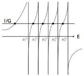
Figure 1: Graphical solution of the equation (5.40)

As can be seen from Fig.1, solutions to this equation for $G=\infty$  can be read off from the $x$ axis. In addition, if needed,  for any $N\geq 1$ the system of equations (5.37a) can be rewritten in a similar BCS-like form if we introduce the renormalized coupling constant $G_{\alpha}$ via

$$G_{\alpha}=G[1+2G\sum\limits_{\beta(\beta\neq\alpha)}^{N}\frac{1}{E_{\beta}-E_{\alpha}}]^{-1}\text{ }$$ (5.41)

so that  now we obtain:

$$F(E_{\alpha})=G_{\alpha}^{-1},\alpha=1,...,N.$$ (5.37b)

This sustem of equations can be solved iteratively, beginning with equation (5.40). There is, however, better way of obtaing these solutions. In view of equations (5.15), (5.16) and (5.23) solutions $\{E_{\alpha}\}$ of (5.37.b) are the roots of the Lame${}^{\prime}-$type function which is  obtained as solution of (5.15). Surprisingly, this fact known to mathematicians for a long time has been recognized in nuclear physics literature only very recently [89].

5.5 Emergence of the Veneziano-like amplitudes  as consistency condition for $N=1$ solutions of the K-Z equations. Recovery of the pion-pion scattering amplitude

Since results for the Richardson-Gaudin (R-G) model are obtainable from the corresponding solutions of the K-Z equations in this subsection we would like to explain why $N=1$ solution of the Bethe-Richardon equations can be linked with the Veneziano-like amplitudes describing the pion-pion scattering. In doing so, we shall by pass the P-F model since, anyway, it is obtainable from the R-G model.

Thus, we begin again with equations (5.10)-(5.11). We would like to look at the special class of solutions of (5.11) for which the parameter $\left|J\right|$ in Verma module (5.19) is equal to one. This corresponds exactly to the case $N=1$. Folloving Varchenko [8], by analogy with (5.16) we introduce the function $\Phi(\mathbf{z},t)$ via

$$\Phi(\mathbf{z},t)=\prod\limits_{1\leq i<j\leq L}(z_{i}-z_{j})^{\dfrac{m_{i}m_{j}}{\kappa}}\prod\limits_{l=1}^{L}(t-z_{l})^{-\dfrac{m_{l}}{\kappa}}.$$ (5.42)

It is a multivalued function at  points of its singularities at $z_{1},...,z_{L}.$ Using this function,  we define the set of 1-forms via

$$\omega_{j}=\Phi(\mathbf{z},t)\frac{dt}{t-z_{j}},\text{ \ }j=1,...,L,$$ (5.43)

and the vector $\mathbf{I}^{(\gamma)}$ of integrals $\mathbf{I}^{(\gamma)}=($I${}_{1},...,$I${}_{L})\equiv(\int\nolimits_{\gamma}\omega_{1},...,\int\nolimits_{\gamma}\omega_{L})$ with $\gamma$ being a particular Pochhammer countour:  a double loop winding around  any two points $z_{\alpha}$, $z_{\beta}$ taken from the set $z_{1},...,z_{L}.$ Deatails can be found in [8,75].

We want now to design the singular Verma module for the K-Z equations using  equation (5.19) and results just presented. Taking into account the following known relations:

$$a)\text{ }ef^{k}v_{m}=k(m-k+1)f^{k-1}v_{m},\text{ and }b)\text{ }hf^{k}v_{m}=(m-2k)f^{k}v_{m}$$

for the Lie algebra $sl_{2}$ also used in Part II, Section 8, and taking into account that in the present ($N=1$) case the basis vectors $f^{J}v_{M}=f^{j_{1}}v_{m_{1}}\otimes\cdot\cdot\cdot\otimes f^{j_{n}}v_{m_{n}}$ acquire the following form: $f^{\mathbf{1}}v_{M}=v_{m_{1}}\otimes\cdot\cdot\cdot\otimes fv_{m_{s}}\otimes\cdot\cdot\cdot\otimes v_{m_{n}},s=1,...,L,$ provided that $m_{i}^{\prime}s$ are the same as in (5.25) (or (5.42)),  the singular vector for such a Verma module is given by

$$w(\gamma)=\sum\limits_{s=1}^{L}I_{s}v_{m_{1}}\otimes\cdot\cdot\cdot\otimes fv_{m_{s}}\otimes\cdot\cdot\cdot\otimes v_{m_{n}}.$$ (5.44)

In view of the Lie algebra relations just introduced, we obtain $e\cdot w=0$ or, explicitly,

$$\sum\limits_{s=1}^{L}m_{s}I_{s}=0.$$ (5.45)

Hence, for a fixed Pochhammer contour $\gamma$ there are $L-1$ independent basis vectors $\{w^{i}\}$. They represent $L-1$ independent solutions of the K-Z equation of the type $k=1$ (or $N=1$). Let now $z_{i}^{\prime}s$ be ordered in such a way that $z_{1}<\cdot\cdot\cdot<z_{L}.$ Furthermore, in view their physical interpretation described in previous section, these $z_{i}^{\prime}s$ can be chosen to be equidistant. Consider then a special set of Pochhamer contours $\{\gamma_{i}\}$   around points $z_{i}$ and $z_{i+1},$ $i=1,2,...,L-1$  and consider the matrix $\mathbf{M}$ made of integrals of the type  $M_{j}^{i}=-\dfrac{m_{j}}{\kappa}\int\nolimits_{\gamma_{i}}\omega_{j}$ then, any ($k=1)-$ type solution $\phi^{i}(i=1,2,...,L-1)$ of the K-Z equation can be represented as

$$\phi^{i}=\sum\limits_{j}M_{j}^{i}w^{j},\text{ }i=1,2,...,L-1.$$ (5.46)

From linear algebra it is known that in order for these K-Z solutions to be independent  we have to require that $\det\mathbf{M}$ $\neq 0.$ The proof of this fact is given in Appendix B. Calculation of the determinant of $\mathbf{M}$ is described in detail in [8] with the result:

$$\det\mathbf{M=\pm}\text{A}\frac{\Gamma(1-\frac{m_{1}}{\kappa})\cdot\cdot\cdot\Gamma(1-\frac{m_{L}}{\kappa})}{\Gamma(1-\frac{\left|M\right|}{\kappa})}$$ (5.47)

with $\pm$A being some known constant and $\Gamma(x)$ being Euler’s gamma function. For $L=2$ without loss of generality one can choose $z_{1}=0$ and $z_{2}=1,$ then  in thus obtained determinant one easily can recognize the Veneziano-type $\pi^{+}\pi^{-}$ scattering amplitude used in the work by Lovelace [90]. We have discussed this amplitude previously in connection with mirror symmetry issues [91]. This time, however, we would like to discuss other topics.

In particular, we notice first that all mesons are made of two quarks. Specifically, we have $u\bar{d}$ for $\pi^{+},d\bar{u}$ for $\pi^{-}$ and $d\bar{d}$ for $\pi^{0}.$ These are very much like the Cooper pairs with $q\bar{q}$  quark pairs contributing to the Bose condensate  which was created as result of spontaneous chiral symmetry breaking. As in the case of more familiar Bose condensate, in addition to the ground state we expect to have a tower of the excited states made of such quark pairs. Experimentally, these are interpreted as more massive mesons. Such excitations are ordered by their energies, angular momentum and, perhaps, by other quantum numbers which can be taken into account if needed. Color confinement postulate makes such a tower infinite. Evidently, the Richardson-Gaudin (R-G) model fits ideally this qualitative picture. Equation (5.40) describes excitations  of such Cooper-like pairs (even in the limit: $G\rightarrow\infty)$ as can be seen from Fig.1. In the P-F model the factor $\tilde{\Omega}_{i}$ plays effectively the role of energy as discussed already in this work and Part II. Therefore, in view of (5.38), it is appropriate to write: $\tilde{\Omega}_{i}=f(E_{i}),$ with $E_{i}$ being the R-G energies. Although the explicit form of such $f-$dependence may be difficult to obtain, for our purposes it is sufficient only to know that such a dependence does exist. This then allows us to make an identification: $\tilde{\Omega}_{i}\rightleftarrows\dfrac{m_{i}}{\kappa}$ consistent with Varchenko’s results, e.g. compare his Theorem 3.3.5 (page 35) with Theorem 6.3.2. (page 90) [8]. But, we had established that $\tilde{\Omega}_{i}$ is an integer, therefore, $\dfrac{m_{i}}{\kappa}$ should be also an integer. This creates some apparent problems. For instance, when $\left|M\right|=\kappa$, the determinant, $\det\mathbf{M,}$ becomes zero implying that solutions of K-Z equation become interdependent. This fact has physical significance to be discussed below and in Section 6. To do so we use some results from our Part I. In particular, a comparison between

$$\sin\pi z=\pi z\prod\limits_{k=1}^{\infty}(1-\left(\frac{k}{z}\right))(1+\left(\frac{k}{z}\right))$$ (5.48)

and

$$\frac{1}{\Gamma(z)}=ze^{-Cz}\prod\limits_{k=1}^{\infty}(1+\left(\frac{k}{z}\right))e^{-\dfrac{z}{k}}$$ (5.49)

where $C$ is some known constant,  tells us immediately that not only $\left|M\right|=\kappa$ will cause $\det\mathbf{M=}0$ but also $\left|M\right|=\kappa(k+1),k=0,1,2,...$ Accordingly, the numerator of (5.47) will create poles whenever $\dfrac{m_{i}}{\kappa}=1.$ Existence of  independent K-Z solutions is not destroyed if, indeed, such poles do occur. These facts allow us to relabel $\dfrac{m_{i}}{\kappa}$ as $\alpha(s)$ (or $\alpha(t)$ or $\alpha(u)$, etc.) as it is done in high energy physics with continuous parameters s, t, u,… replacing discrete i’s, different for different $\Gamma$ functions in the numerator of  (5.47). In the simplest case, this allows us to reduce the determinant in (5.47) to the form used by Lovelace, i.e.

$$\det\mathbf{M=-}\lambda\frac{\Gamma(1-\alpha(s))\Gamma(1-\alpha(t))}{\Gamma(1-\alpha(s)-\alpha(t))}.$$ (5.50)

If, as usual, we parametrize $\alpha(s)=\alpha(0)+\alpha^{\prime}s$, then equation $1=\alpha(s)+\alpha(t)$ causes the $\det\mathbf{M}$ to vanish. This also fixes parameter $\alpha(0)$: $\alpha(0)=1/2.$ This result was obtained  by Adler long before sting theory emerged and is known as Adler’s  selfconsistency condition [92]. With such ”gauge fixing”, one can fix the slope $\alpha^{\prime}$ as well  if one notices that the experimental data allow us to make a choice: $1=\alpha(m_{\rho}^{2}).$This leads to: $\alpha^{\prime}=\frac{1}{2m_{\rho}^{2}}\sim 0.885(Gev^{-2})$ in accord with observations..

The obtained  results are not limited to study of excitations of just one ”supeconducting” pair of quarks. In princile, any finite amount of such pairs can be studied. In such a case the result for $\det\mathbf{M}$ becomes considerably more complicated but the connections with one dimensional magnets become even more explicit. We plan to discuss these issues in future publications.

6 Discussion.  Unimaginable ubiquity of Veneziano-like amplitudes in Nature

6.1 General remarks

In the Introduction, following Heisenberg, we posed the question: Is combinatorics of observational data sufficient for recovery of the underlying unique microscopic model? That is, can we have the complete understanding of such a model based on information provided by combinatorics? As we demonstrated, especially in Section 4, this task is impossible to accomplish without imposing additional constraints  which, normally, are not dictated by the combinatorics only. In Section 5 we demonstrated that, even accounting for such constraints, the obtained results could be in conflict with rigorous mathematics. Last but not the least, since Veneziano amplitudes gave birth to string theory one can pose a question: Is these Veneziano (or Veneziano-like) amplitudes, perhaps corrected to account for particles with spin, contain enough information (analytical, number-theoretic, combinatorial, etc.) that allows restoration of the underlying microscopic model uniquely?  The answer is: ”No”!  In the rest of this section we explain why.

6.2 Random fragmentation and coagulation processes and the Dirichlet distribution

We begin by recalling some known facts from the probability theory. For instance, we recall that the stationary Maxwell distribution for velocities of particles in the gas is just of Gaussian-type.  It can be obtained  as a stationary solution of the Boltzmann’s dynamical equation maximizing Boltzmann’s entropy.The question arises: Is it possible to find (discrete or continuous) dynamical equations which will provide known probability laws as stable stationary solutions? This task will involve finding of  dynamical equations along with the corresponding Boltzmann-like entropies which  will reach their maxima at respective equilibria for these dynamical equations. We are certainly not in the position in this closing section of our paper to discuss this problem in full generality. Instead, we focus our attention only on processes wihich are described by the so called Dirichlet distributions.These originate from the integral (equation (2.8) of Part I) attributed to Dirichlet, that is

$$\mathcal{D}(x_{1},...,x_{n+1})=\idotsint\limits_{\begin{subarray}{c}u_{1}\geq 0,...,\text{ }u_{n}\geq 0\\ u_{1}+\cdot\cdot\cdot+u_{n}\leq 1\end{subarray}}u_{1}^{x_{1}-1}\cdot\cdot\cdot u_{n}^{x_{n}-1}(1-u_{1}-\cdot\cdot\cdot-u_{n})^{x_{n+1}-1}du_{1}\cdot\cdot\cdot du_{n}.$$ (6.1)

A random vector $(\mathbf{X}_{1},...,\mathbf{X}_{n})\in\mathbf{R}^{n}$  such that $\mathbf{X}_{i}\geq 0$ $\forall i$ and $\sum\limits_{i=1}^{n}$  $\mathbf{X}_{i}$ $\mathbf{=}1$ is said to be Dirichlet distributed with parameters ($x_{1},...,x_{n};x_{n+1})$ [nevzorov] if the probability density function for $(\mathbf{X}_{1},...,\mathbf{X}_{n})$ is given by

$$P_{\mathbf{X}_{1},...,\mathbf{X}_{n}}(u_{1},...,u_{n}) = \frac{\Gamma(x_{1}+\cdot\cdot\cdot+x_{n+1})}{\Gamma(x_{1})\cdot\cdot\cdot\Gamma(x_{n+1})}u_{1}^{x_{1}-1}\cdot\cdot\cdot u_{n}^{x_{n}-1}(1-\sum\limits_{i=1}^{n}u_{i})^{x_{n+1}-1}$$ (57)

$$\equiv \frac{\Gamma(x_{1}+\cdot\cdot\cdot+x_{n+1})}{\Gamma(x_{1})\cdot\cdot\cdot\Gamma(x_{n+1})}u_{1}^{x_{1}-1}\cdot\cdot\cdot u_{n}^{x_{n}-1}u_{n+1}^{x_{n+1}-1},\text{ provided that \ }u_{n+1}$$

$$= 1-u_{1}-\cdot\cdot\cdot-u_{n}\TCItag{6.2}$$

To get some physical feeling of just defined distribution, we notice the following peculiar aspects of this distribution. First, for any discrete distribution, we know that the probability $p_{i}$ must be normalized, that is $\sum\nolimits_{i}p_{i}=1.$ Thus, the Dirichlet distribution is dealing with averaging of the probabilities! Or, better, is dealing with the problem of effectively selecting the most optimal discrete probability. The most primitive of these probabilities is the binomial probability given by

$$p_{m}=\left(\begin{array}[]{c}n\\ m\end{array}\right)p^{m}(1-p)^{n-m},\text{ \ }m=0,1,2,....,n\text{.}$$ (6.3)

If $X$ is random variable obeying this law of probability then, the expectation  $E(X)$ is calculated as

$$E(X)=\sum\limits_{m=1}^{n}mp_{m}=np\equiv\mu.$$ (6.4)

Consider such a distribution in the limit: $n\rightarrow\infty.$ In this limit, if we write $p=\mu/n$ , then the Poisson distribution is obtained as

$$p_{m}=\frac{\mu^{m}}{m!}e^{-\mu}.$$ (6.5)

Next, we notice that $m!=\Gamma(m+1),$ furthermore, we replace $m$ by real valued variable $\alpha$ and $\mu$ by $x$. This allows us to introduce the gamma distribution  with exponent $\alpha$ whose probability density is

$$p_{X}(x)=\frac{1}{\Gamma(\alpha)}x^{\alpha-1}e^{-x}$$ (6.6)

for some gamma distributed random variable $X$. Finally, we would like to demonstrate now how the Dirichlet distribution can be represented through gamma distributions. Since the gamma distribution originates from the Poisson distribution, sometimes in literature the Dirichlet distribution is called the Poisson-Dirichlet (P-D) distribution [14]. To demonstrate connection between the Dirichlet and gamma distributions is relatively easy. Following Kingman [14], consider a set of positive independent gamma distributed random variables: $Y_{1},...,Y_{n+1}$ with exponents $\alpha_{1},...,\alpha_{n+1}.$ Furthermore, consider  $Y=Y_{1}+\cdot\cdot\cdot+Y_{n+1}$ and construct  a vector u with components: $u_{i}=\frac{Y_{i}}{Y}$. Then, since $\sum\nolimits_{i=1}^{n+1}u_{i}$ =$1,$ the components of this vector are Dirichlet distributed and, in fact, independent of $Y$.  Details are given in Appendix C.

Such described Dirichlet distribution is an equilibrium measure in various fields ranging from spin glasses to computer science, from linguistics to genetics, from forensic science to economics, etc. Many useful references involving these and other applications can be found in [9-11]. Furtheremore,  most of fragmentation and coagulation processes involve the P-D distribution as their equilibrium measure. Some applications of general theory of these processes to to nuclear and particle physics were initiated in a series of papers by Mekjian, e.g. see [12] and references therein. To avoid duplications, we would like to rederive some of Mekjian results differently in order to exibit their connections with previous sections.

6.3 The Ewens sampling formula and Veneziano amplitudes

This formula was discussed by Mekjian in [94] without any reference to P-D distribution. It is discussed in many other places, including Ewens own monograph [95]. Our exposition follows work by Watterson [96] where he considers a simple  P-D average of  monomials of the type generated by the individual terms in the expansion

$$\mathbf{u}^{n}=(u_{1}+\cdot\cdot\cdot+u_{k})^{n}=\sum\limits_{n=(n_{1},...,n_{k})}\frac{n!}{n_{1}!n_{2}!\cdot\cdot\cdot n_{k}!}u_{1}^{n_{1}}\cdot\cdot\cdot u_{k}^{n_{k}}.$$ (6.7)

Such type of expansion was used in Part I (equations (2.9),(2.11)) for calculation of multiparticle Veneziano amplitudes. Not surprisingly, Watterson’s calculation also results in the multiparticle Veneziano amplitude which upon multiplication by some combinatorial factor in a well defined limit produces the Ewens sampling formula playing  a major role in genetics.  Although in Appendix D we reproduce the Ewens sampling formula without use of the P-D distribution, Kingman [98] demonstrated that ”A sequence of populations has the Evens sampling property if and only if it has the P-D limit”. Hence, we expect that our readers will consult the Appendix D prior to reading of what follows. Furthermore, since the vector u is P-D distributed, it is appropriate to mention at this point that equation (6.7) genetically represents the Hardy-Weinberg law [95] for mating species. Hence, the Ewens sampling formula provides a refinement of this law accounting for mutations.

Considear a special case of (6.2) for which $x_{1}=x_{2}=\cdot\cdot\cdot x_{K+1}=\varepsilon$ and let $\varepsilon=\theta/K$ with parameter $\theta$ to be defined later. Then, (6.2) is converted to

$$P_{\mathbf{X}_{1},...,\mathbf{X}_{K}}(u_{1},...,u_{K}) \equiv \phi_{k}(\mathbf{u})=\frac{\Gamma((K+1)\varepsilon)}{\left[\Gamma(\varepsilon)\right]^{K+1}}\prod\limits_{i=1}^{K+1}u_{i}^{\varepsilon-1}\text{ provided that }1$$

$$= \sum\nolimits_{i=1}^{K+1}u_{i}\TCItag{6.8}$$ (60)

In view of (6.7), consider an average $P(n_{1},...,n_{K})$ over the simplex $\Delta$ (defined by $\sum\nolimits_{i=1}^{K+1}u_{i}=1)$ given by

$$P(n_{1},...,n_{K})=\frac{n!}{n_{1}!n_{2}!\cdot\cdot\cdot n_{K}!}\idotsint\limits_{\Delta}u_{1}^{n_{1}}\cdot\cdot\cdot u_{K}^{n_{K}}\phi_{k}(\mathbf{u})du_{1}\cdot\cdot\cdot du_{K}.$$ (6.9)

A straightforward calculation produces:

$$P(n_{1},...,n_{K})=\frac{n!}{n_{1}!n_{2}!\cdot\cdot\cdot n_{K}!}\frac{\Gamma((K+1)\varepsilon)}{\left[\Gamma(\varepsilon)\right]^{K+1}}\prod\limits_{i=1}^{K}\frac{\Gamma(\varepsilon+n_{i})}{\Gamma((K+1)\varepsilon+n)}$$ (6.10)

to be compared with (5.47). Evidently, the parameter $\varepsilon$ can be identified with $\kappa$ in $(5.47)$ and, if we select $\theta$ to be a positive integer, then by replacing $n_{i}^{\prime}s$ with $-n_{i}^{\prime}s$ we reobtain  back (5.47) (up to a constant). To obtain the Ewens sampling formula (equation (D.6)) from (6.10) few additional steps are required. These are: a) we have to let $K\rightarrow\infty$ while allowing many of $n_{i}^{\prime}s$ in (6.7) to become zero (this explains meaning of the word ”sampling”), b) we have to order remaining $n_{i}^{\prime}s$  in such a way that $n_{(1)}\geq n_{(2)}\geq\cdot\cdot\cdot\geq n_{(k)}>0,0,...,0,$ c) we have to cyclically order the remaining $n_{i}^{\prime}s$ in a way explained in the Appendix D by introducing $c_{i}^{\prime}s$ as numbers of remaining $n_{(i)}^{\prime}s$  which are equal to $i$. That is we have to make a choice between representing $r=\sum\nolimits_{i=1}^{k}n_{(i)}$ or $r=\sum\nolimits_{i=1}^{r}ic_{i}$ under condition that $\ k=\sum\nolimits_{i=1}^{r}c_{i},$ d) finally, just like in the case of Bose (Fermi) statistics, we have to multipy the r.h.s. of (6.10) by the obviously looking combinatorial factor $M=K!/[(c_{1}!\cdot\cdot\cdot c_{r}!)((K-k)!]$. Under such conditions we obtain: $\Gamma((K+1)\varepsilon)\simeq\Gamma(\theta),\Gamma((K+1)\varepsilon+r)=\Gamma(\theta+r),\frac{\Gamma(\varepsilon+n_{(i)})}{n_{(i)!}}=\frac{1}{n_{(i)}}.$ Less trivial is the result: $K!/[(K-k)!\left[\Gamma(\varepsilon)\right]^{k}]\rightarrow\theta^{k}.$ Evidently, the factor $\dfrac{n!}{n_{1}!n_{2}!\cdot\cdot\cdot n_{K}!}$  in (6.10) now should be replaced by $\dfrac{r!}{n_{(1)}\cdot\cdot\cdot n_{(k)}}.$ Finally, a moment of thought causes us to replace $n_{(i)}^{\prime}s$ by $\ i^{c_{i}}$ in order to arrive at the Ewens sampling formula:

$$P(k;n_{(1)},...,n_{(k)})=\frac{r!}{[\theta]^{r}}\prod\limits_{i=1}^{r}\frac{\theta^{c_{i}}}{i^{c_{i}}c_{i}!}$$ (6.11)

in agreement with (D.6). This derivation was made without any reference to genetics and is completely model-independent. To demonstrate connections with high energy physics in general and with Veneziano amplitudes in particular,  we would like to explain the rationale behind this formula using absolute minimum facts from genetics.

Genetic information is stored in genes. These are some segments (locuses) of the double stranded DNA molecule. This fact allows us to think about the DNA molecule as a world line for mesons made of a pair of quarks.  Phenomenologically, the DNA is essentially the chromosome. Humans and many other species are diploids. This means that they need for their reproduction (meiosis) two sets of chromosomes-one from each parent.  Hence, we can think of meiosis as process analogous to the meson-meson scattering.  We would like to depict this process graphically to emphasize the analogy. Before doing so we need to make few remarks. First, the life cycle for diploids is rather bizarre. Each cell of a grown up organism contains 2 sets of chromosomes. The maiting, however, requires this rule to be changed. The gametes (sex cells) from each parent carry only one set of chromosomes (that is such cells are haploid !). The existence of 2 sets of chromosomes makes individual organism unique because of the following. Consider, for instance, a specific trait, e.g. ”tall” vs ”short”. Genetically this property in encoded in some gene. A particular realization of the gene (causing the organism to be, say, tall) is called ”allele”. Typically, there are 2 alleles -one for each of the chromosomes in the two chromosome set. For instance, T and t (for ”tall” and ”short”), or T and T or t and t or, finally, t and T (sometimes order matters). Then, if father donates 50% of T cells and 50% of t cells and mother is doing to do the same, the offspring is likely going to have either TT composition with probability 1/4, or tt (with probability 1/4) or tT (with probability 1/4) and, finally, tt with probability 1/4. But, one of the alleles is usually dominant (say, T) so that we will see 3/4 of tall people in the offspring and 1/4 short.  What we just described is the essence of the Hardy-Weinberg law based, of course, on the original works by Mendel. Details can be found in genetics literature [95].

Let us concentrate our attention on a particular locus so that the genetic character(trait) of a particular individual is described by specifying its two genes at that locus. For $N$ individuals in the population there are $2N$ chromosomes containing such a locus. For each allele, one is interested in knowing the proportion of $2N$ chromosiomes at which the gene is realized as this allele. This gives a probability distribution over the set of possible alleles which describes a genetic make-up of the population (as far as we are  only looking at some specific locus). The problem now is to model the dynamical process by which this distribution changes in time from generation to generation accounting for mutations and selection (caused by the environment). Mutation can be caused just by chane of one nucleotide along the DNA strand. Normally, the mutant allele is independent of its parent since once the mutation took place it is very unlikely that the corrupt message means anything at all. Hence, the mutant can be either ”good” (fit) or ”bad” (unfit) for life and its contribution can be ignored. If $u$ is the probability of mutation per gene per generation then, the parameter $\theta=4Nu$ in (6.11). With this information , we are ready to restore the rest of the genetic content of Watterson’s paper [96]. In particular, random P-D variables $\mathbf{X}_{1},\mathbf{X}_{2},...,\mathbf{X}_{K}$ denote the allele relative frequences in a population consisting of $K$ alleles. Evidently, by construction, they are Dirichlet-distributed. Let $K\rightarrow\infty$ and let $k$ be an experimental sample of representative frequencies $k\ll K.$ The composition of such a sample will be random, both because of the nature of the sampling process and because the population itself is subject to random fluctuations. For this reason we averaged the Hardy-Weinberg distribution (6.7) over the P-D distribution in order to arrive at the final result (6.11). This result is an equilibrium result. Its experimental verification can be found in [ewens, watterson2]. It is of interest to arrive at it dynamically  along the lines discussed in Section 6.2. This is accomplished in the next subsection but in a different context.  Based on the facts just discussed and comparing them with those of Section 2 and Part II, it should be clear that both genetics and physics of meson scattering have the same combinatorial origin. All random processes involving decompositions $r=\sum\nolimits_{i=1}^{k}n_{(i)}$ (or $r=\sum\nolimits_{i=1}^{r}ic_{i}$) are the P-D processes [9].

To conclude this subsection, we would like to illustrate graphically why genetics and physics of hadrons have many things in common. This is done with help of the figures 2 through 4.

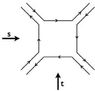
Figure 2: The simplest duality diagram describing meson-meson scattering [99]. The same picture  describes ”collision” of two parental DNA’s during meiosis and can be seen directly under the electron microscope. E.g.see Fig.2.3 in [100], page 18.

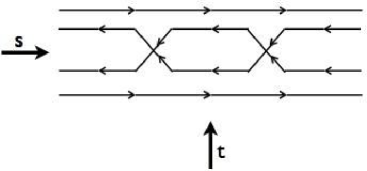
Figure 3: Non -planar loop Pomeron diagram for meson-meson scattering [101]. The same diagram describe homologous DNA recombination, e.g. see fig.2.2 in [100], page 17.

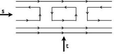
Figure 4: Planar loop meson-baryon scattering duality diagram.The same diagram describes the interaction $scattering$ between the triple and double stranded DNA helices [102]

6.4 Stochastic models for  second order chemical reaction kinetics involving Veneziano-like amplitudes

In Section 4 and Appendix A we demonstrated the impotant role of  the ASEP in elucidating the correct physics. Historically, however, long before the ASEP was formulated,  the role of stochastic processes in chemical kinetics  was already recognized. A nice summary is contained in the paper by McQuarrie [103]. The purpose of this subsection is to connect the results in chemical kinetics with those in genetics in order to reproduce Veneziano (or Veneziano-like) amplitudes as an equilibrium measures for the underlying chemical/biological processes.

Following Darvey et al [104] we consider a chemical reaction $A+B\begin{array}[]{c}k_{1}\\ \rightleftarrows\\ k_{-1}\end{array}C+D$ analogous to the meson-meson scattering processes which triggered the discovery of  the Veneziano amplitudes. Let the respective concentrations of the reagents be $a,b,c$ and $d$. Then, according to rules of chemical kinetics, we obtain the following ”equation of motion”

$$\frac{da}{dt}=-k_{1}ab+k_{-1}cd.$$ (6.12)

This equation has to be supplemented with the initial condition. It is obtained by accounting for the mass conservation. Specifically, let the initial concentrations of reagents be respectively as $\alpha=A(0),\beta=B(0),\gamma=C(0)$ and $\delta=D(0).$ Then, evidently, $\alpha+\beta+\gamma+\delta=a+b+c+d,$  provided that  for all times $a\geq 0,b\geq 0,c\geq 0$ and $d\geq 0$ (to be compared with equations (2.1), (2.3)). Accounting for these facts,  equation (6.12) can be rewritten as

$$\frac{da}{dt}=(k_{-1}-k_{1})a^{2}-[k_{1}(\beta-\alpha)+k_{-1}(2\alpha+\gamma+\delta)]a+k_{-1}(\alpha+\gamma)(\alpha+\beta).$$ (6.13)

Theis is thus far is standard result of chemical kinetics. The new element emerges when one claims that the the variables $a,b,c$ and $d$ are random but are still subject to the mass conservation. Then, as we know already from previous subsections, we are dealing with the P–D-type process. New element now lies in the fact that this process is dynamical. Following Kingman [105] we would like to formulate it in precise mathematical terms. For this purpose, we introduce the vector p(t)=(p₁(t),…, p_k(t)) such that it moves randomly on the simplex $\Delta$ defined by

$$\Delta=\{\mathbf{p}(t);p_{j}\geq 0,\sum\nolimits_{i=1}^{k}p_{i}=1\}$$ (6.14)

In our case the possible states of the system at time $t$ which could lead to a new state specified by $a,b,c,d$ at time $t+\Delta t$ involving not more than one transformation in the time interval $\Delta t$ are [104]

$$\left(\begin{array}[]{cccc}a+1&b+1&c-1&d-1\\ a-1&b-1&c+1&d+1\\ a&b&c&d\end{array}\right).$$ (6.15)

In writing this matrix, following [104], we assume that random variables $a,b,c$ and $d$ are integers, just like in (2.3),(2.4). By analogy with equations of motion of Appendix A,  using (6.15) we obtain,

$$P(a,b,c,d;t+\Delta t)-P(a,b,c,d;t) = [k_{1}(a+1)(b+1)P(a+1,b+1,c-1,d-1;t)$$ (67)

$$+k_{-1}(c+1)(d+1)P(a-1,b-1,c+1,d+1;t)$$

$$-(k_{1}ab+k_{-1}cd)P(a,b,c,d;t)]\Delta t+O(\Delta t)\TCItag{6.16}$$

In view of the fact that the motion is taking place on the simplex $\Delta$ it is sufficient to look at the stochastic dynamics of just one variable, say, $a$ (very much like in the deterministic equation (6.13). This replaces (6.16) by the following result:

$$\frac{d}{dt}P_{a}(t) = k_{1}[(a+1)(a+1+\beta-\alpha)P_{a+1}(t)+k_{-1}[(\gamma+\alpha-a+1)(\delta+\alpha-a+1)P_{a-1}(t)$$

$$-[k_{1}a(\beta-\alpha+a)+k_{-1}(\gamma+\alpha-a)(\delta+\alpha-a)]P_{a}(t);\text{ \ provided that}$$

$$\text{\ \ }P_{\alpha}(0) = 1,\text{ \ \ }\alpha=a\text{ and }P_{\alpha}(0)=0\text{ if }a\neq\alpha.\TCItag{6.17}$$ (68)

To solve this equation we introduce the generating function $G(x,t)$ via

$$G(x,t)=\sum\limits_{a=0}P_{a}(t)x^{a}$$

and use this function in (6.17) to obtain the following Fokker–Plank-type equation

$$\frac{\partial}{\partial t}G(x,t) = x(1-x)(k_{1}-xk_{-1})\frac{\partial^{2}}{\partial x^{2}}G+(1-x)[k_{1}(\beta-\alpha+1)$$ (69)

$$+k_{-1}(2\alpha+\gamma+\delta-1)x]\frac{\partial}{\partial x}G$$

$$-k_{-1}(\alpha+\gamma)(\alpha+\delta)(1-x)G(x,t)\TCItag{6.18}$$

This equation admits separation of variables: $G(x,t)=S(x)T(t)$ with solution for $T(t)$ in the expected form: $T(t)=exp(-\lambda_{n}k_{1}t)$ leading to the equation for $S(x)$

$$x(1-x)(1-Kx)\frac{d^{2}}{dx^{2}}S(x)+[\beta-\alpha+1+K(2\alpha+\gamma+\delta-1)x](1-x)\frac{d}{dx}S-[K(\alpha+\gamma)(\alpha+\beta)(1-s)-\lambda_{n}]S(x)=0$$ (6.19)

This equation is of Lame-type discussed in Section 5 (e.g.see (5.15)) and, therefore, its solution should be a polynomial in $x$ of degree at most $\varpi$ where $\varpi$ should be equal to the minimum of ($\alpha+\gamma,\alpha+\delta,\beta+\gamma,\delta+\delta).$ As in quantum  mechanics, this implies that the spectrum of eigenvalues $\lambda_{n}$ is  discrete, finite and nondegenerate. Among these eigenvalues there must be $\lambda_{0}=0$ since such an eigenvalue corresponds to the time-independent solution of (6.19) corresponding to true equilibrium. Hence, for this case we obtain instead of (6.19) the following final result:

$$x(1-Kx)\frac{d^{2}}{dx^{2}}S(x)+[\beta-\alpha+1+K(2\alpha+\gamma+\delta-1)x]\frac{d}{dx}S-[K(\alpha+\gamma)(\alpha+\beta)]S=0$$ (6.20)

where $K=k_{-1}/k_{1}.$ This constant can be eliminated from (6.20) if we rescale $x:x\rightarrow Kx.$ After this, equation acquires the standard hypergeometric form

$$x(1-x)\frac{d^{2}}{dx^{2}}S(x)+[\beta-\alpha+1+(2\alpha+\gamma+\delta-1)x]\frac{d}{dx}S(x)-(\alpha+\gamma)(\alpha+\beta)S(x)=0.$$ (6.21)

In [105] Kingman obtained the Fokker-Planck type equation analogous to our (6.18) describing the dynamical peocess whose stable equilibrium is described by (6.21) ( naturally, with different coefficients) and leads to the P-D distribution (6.2) essential for obtaining Ewens sampling formula. Instead of reproducing his results in this work, we would like to connect them with results of our Section 5.  For this purpose,we begin with the following observation.

6.4.1  Quantum mechanics, hypergeometric functions and P-D distribution

In our works [2,3] we  provided detailed explanation of the fact  that all  exactly solvable 2-body quantum mechanical problems involve different kinds of special functions obtainable from the Gauss hypergeometric funcftion whose integral representation is given by

$$F(a,b,c;z)=\frac{\Gamma(c)}{\Gamma(b)\Gamma(c-b)}\int\limits_{0}^{1}t^{b-1}(1-t)^{c-b-1}(1-zt)^{-a}dt.$$ (6.22)

As it is well known from quantum mechanics, in the case of disctete spectrum all quantum mechanical problems involve orthogonal polynomials.The question then arises: under what conditions on coefficients ($a,b$ and $c$) infinite hypergeometric series whose integral representation is given by (6.22) can be reduced to a finite polynomial? This happens, for instance, if we impose the quantization condition: $-a=0,1,2,....$ In such a case we can write $(1-zt)^{-a}=\sum\nolimits_{i=1}^{-a}(_{i}^{-a})(-1)^{i}(zt)^{i}$  and use this finite expansion in (6.22). In view of (6.2) we obtain the convergent generating function for the Dirichlet distribution (6.2). Hence, all  known quantum mechanical problems involving discrete spectrum are effectively examples of the P-D stochasic processes. Next, we are interested in the following. Given this fact, can we include the determinantal formula (5.47) into this quantization scheme?  Very fortunately, this can be done. as explained in the next subsection..

6.4.2 Hypergeometric functions, Kummer series expansions and Veneziano amplitudes

In view of just introduced quantization condition, the question arises: is this the only condition reducing the hypergeometric function to a polynomial ? More broadly: what conditions on coefficients $a,b$ and $c$  should be imposed so that the function $F(a,b,c;z)$ becomes a polynomial? The answer to this question was provided by Kummer in the first half of 19th century [107]. We would like to summarize his results and to connect them with determinantal formula (5.43). By doing so we shall reobtain Veneziano amplitudes for  chemical process described by (6.21).

According to general theory of hypergeometric equations [107], the infinite series for hypergeometric function degenerates to a polynomial if one of the numbers

$$a,b,c-a\text{ or \ }c-b$$ (6.23)

is an integer. This condition is equivalent to a condition that, at least one of eight numbers $\pm(c-1)\pm(a-b)\pm(a+b-c)$ is an odd number. According to general theory of hypergeometric functions of multiple arguments summarized in Section 5, the $k=1$ -type solutions can be obtained using 1-forms (5.43) accounting for  singular module constraint (5.45). in the form given by equation (5.42). In the case of Gauss-type hypergeometric functions, relations of the type given by (5.45) were obtained by Kummer who found 24 interdependent solutions. Evidently, this number is determined by the number of independent Pochhamer contours [107]. Therefore, among these he singled out 6 (generating these 24) and among these 6 he established that every 3 of them are related to each other via equation of the type (5.45).

Let us denote these 6 functions as $u_{1},...,u_{6}$ then, we can represent, say, $u_{2}$ and $u_{6}$ using $u_{1}$ and $u_{5}$ as basis set. We can do the same with $u_{1}$ and $u_{5}$ by representing them through $u_{2}$ and $u_{6}$ and, finally, we can connect $u_{3}$ and $u_{4}$ with $u_{1}$ and $u_{5}.$ Hence, it is sufficient to consider, say, $u_{2}$ and $u_{6}.$ We obtain,

$$\left(\begin{array}[]{c}u_{2}\\ u_{6}\end{array}\right)=\left(\begin{array}[]{cc}M_{1}^{1}&M_{2}^{1}\\ M_{1}^{2}&M_{2}^{2}\end{array}\right)\left(\begin{array}[]{c}u_{1}\\ u_{5}\end{array}\right),$$ (6.24)

with $M_{1}^{1}=\dfrac{\Gamma(a+b-c+1)\Gamma(1-c)}{\Gamma(a+1-c)\Gamma(b-c+1)};$ $M_{2}^{1}=\dfrac{\Gamma(a+b+1-c)\Gamma(c-1)}{\Gamma(a)\Gamma(b)};M_{1}^{2}=\dfrac{\Gamma(c+1-a-b)\Gamma(1-c)}{\Gamma(1-a)\Gamma(1-b)};M_{2}^{2}=\dfrac{\Gamma(c+1-a-b)\Gamma(c-1)}{\Gamma(c-a)\Gamma(c-b)}.$ The determinant of this matrix becomes zero if either two rows or two columns become the same. For instance, we obtain:

$$\dfrac{\Gamma(a)\Gamma(b)}{\Gamma(c-1)}=\dfrac{\Gamma(a-c+1)\Gamma(b-c+1)}{\Gamma(1-c)}\text{ and }\frac{\Gamma(c-a)\Gamma(c-b)}{\Gamma(c-1)}=\frac{\Gamma(1-a)\Gamma(1-b)}{\Gamma(1-c)}.$$ (6.25)

For $c=1$ we obtain an identity. From [darvey] we find that (6.21) admits 2 independent solutions:

$$S(x)=\left\{{}\right.\frac{\text{either }F(-\alpha-\gamma,-\alpha-\delta,\beta-\alpha+1;Kx),\text{ for }\beta\geq\alpha\text{ }}{\text{or }\left(Kx\right)^{\alpha-\beta}F(-\beta-\gamma,-\beta-\delta,\alpha-\beta+1;Kx),\text{ for }\beta\leq\alpha\text{ .}}$$ (6.26)

Hence, the condition $c=1$  in (6.25) causes two solutions for $S(x)$ to degenerate into one polynomial solution, provided that we make an identification: $\beta=\alpha$ in (6.26). Notice that  to obtain this result there is no need to impose an extra condition: $a=b$ (or, in our case, which is the same as $\gamma=\delta).$

This makes sence physically both in chemistry and in high energy physics. In the case of high energy physics, if the Veneziano amplitudes are used for description of, say, $\pi\pi$ scattering, in Part I (page 54) it is demonstrated that processes for which ”concentrations ”$a=b$ cause this amplitude to vanish. The Veneziano condition: $a+b+c=-1((1.5)$ of Part I) has its analog in chemistry where it plays the same role, e.g. of mass conservation. In the present case we have $\alpha+\beta+\gamma+\delta=const$ and the Veneziano-like amplitude obtainable from (6.25),(6.26) is given now by

$$V_{c}(a,b)=\frac{\Gamma(-\alpha-\gamma)\Gamma(-\alpha-\delta)}{-c\Gamma(-c)}\mid_{c=1}$$ (6.27)

In view of known symmetry of the hypergeometric function: $F(a,b,c;x)=F(b,a,c;x)$, we also have: $V_{c}(b,a)=V_{c}(a,b).$ This is compatible with the symmetry for Veneziano amplitude. Combining (5.47) with (6.27) we have the following options: a) $\alpha=0,\gamma=1,\delta=1,2,...;b)$ $\alpha=1,\gamma=0,\delta=0,1,2,...$ These conditions are compatible with those in (1.19) of Part I for Veneziano amplitudes. Finally, in view of (6.22), these are quantization conditions for resonances as required..

A. Basics of ASEP    

A.1. Equations of motion and spin chains

The one dimensional asymmetric simple exclusion process (ASEP) had been studied for some time [108]. The purpose of this Appendix is to summarize the key features of this process which are of immediate relevance to the content of this paper. To this purpose, following Schütz [109], we shall briefly describe the ASEP with sequential updating. Let $B_{N}:=\{x_{1},...,x_{N}\}$ be a set of sites of one dimensional lattice arranged at time $t$ in such a way that $x_{1}<x_{2}$ $<\cdot\cdot\cdot<x_{N}$. It is expected that each time update will not destroy this order.

Consider first the simplest case of $N=1$. Let $p_{R}$ $(p_{L})$ be the probability of a particle located at the site $x$ to move to the right (left) then, after transition to continuous time, the master equation for the probability $P(x;t)$ can be written as follows

$$\frac{\partial}{\partial t}P(x;t)=p_{R}P(x-1;t)+p_{L}P(x+1;t)-P(x;t).$$ (A.1)

Assuming that $P(x;t)=\exp(-\varepsilon t)P(x)$ so that that

$P(x;t)=\int\limits_{0}^{2\pi}dp\exp(-\varepsilon t)f(p)\exp(ipx),$ $p\in[0,2\pi),$ we obtain the dispersion relation for the energy $\varepsilon(p):$

$$\varepsilon(p)=p_{R}(1-e^{-ip})+p_{L}(1-e^{ip}).$$ (A.2)

The initial condition $P(x;0)=\delta_{x,y}$ determines $f(p)=e^{-ipy}/2\pi$ and yields finally

$$P(x;t\shortmid y;0)=\frac{1}{2\pi}\int\limits_{0}^{2\pi}dpe^{-\varepsilon(p)t}e^{-ipy}e^{ipx}=e^{-(q+q^{-1})Dt}q^{x-y}I_{x-y}(2Dt),$$ (A.3)

where $q=\sqrt{p_{R}/p_{L}}$, $D=\sqrt{p_{R}p_{L}}$ and $I_{n}(2Dt)$ is the modified Bessel function. These results can be easily extended to the case $N=2$. Indeed, for this case  we obtain the following equation of motion

$$\varepsilon P(x_{1},x_{2}) = -p_{R}(P(x_{1}-1,x_{2})+P(x_{1},x_{2}-1)-2P(x_{1},x_{2}))$$ (76)

$$-p_{L}(P(x_{1}+1,x_{2})+P(x_{1},x_{2}+1)-2P(x_{1},x_{2}))\TCItag{A.4}$$

which should be suppllemented by the boundary condition

$$P(x,x+1)=p_{R}P(x,x)+p_{L}P(x+1,x+1)\text{ }\forall x.$$ (A.5)

Imposition of this boundary condition allows us to look for a solution of (A.4) in the (Bethe ansatz) form

$$P(x_{1},x_{2})=A_{12}e^{ip_{1}x_{1}}e^{ip_{2}x_{2}}+A_{21}e^{ip_{2}x_{1}}e^{ip_{1}x_{2}}$$ (A.6)

yielding $\varepsilon(p_{1},p_{2})=\varepsilon(p_{1})+\varepsilon(p_{2}).$ Use of the boundary condition (A.5) fixes the ratio (the S-matrix) $S_{12}=A_{12}/A_{21}$ as follows:

$$S(p_{1},p_{2})=-\frac{p_{R}+p_{L}e^{ip_{1}+ip_{2}}-e^{ip_{1}}}{p_{R}+p_{L}e^{ip_{1}+ip_{2}}-e^{ip_{2}}}.$$ (A.7)

To connect this result with the quantum spin chains, we consider the case of symmetric hopping first. In this case we have $p_{R}=p_{L}=1/2$ so that (A.7) is reduced to

$$S_{XXX}(p_{1},p_{2})=-\frac{1+e^{ip_{1}+ip_{2}}-2e^{ip_{1}}}{1+e^{ip_{1}+ip_{2}}-2e^{ip_{2}}}$$ (A.8)

from which we can recognize the $S$ matrix for XXX spin 1/2 Heisenberg ferromagnet [67]. If $p_{R}\neq p_{L}$, to bring (A.7) in correspondence with the spin chain $S-$ matrix requires additional efforts. Following Gwa and Spohn [110] we replace the complex numbers $e^{ip_{1}}$ and $e^{ip_{2}}$ in (A.7) respectively by z₁ and z${}_{2}.$ In such a form  (A.7) exactly  coincides with the S-matrix  obtained by Gwa and Spohn. After this we can rescale z_i $(i=1,2)$ as follows: $z_{i}=\sqrt{\frac{q}{p}}\tilde{z}_{i}.$ Substitution of such an asatz into (A.7) leads to the result

$$S_{XXZ}(\tilde{z}_{1},\tilde{z}_{2})=-\frac{1+\tilde{z}_{1}\tilde{z}_{2}-2\Delta\tilde{z}_{1}}{1+\tilde{z}_{1}\tilde{z}_{2}-2\Delta\tilde{z}_{2}},$$ (A.9)

provided that $2\Delta=1/\sqrt{p_{L}p_{R}}$. For $p_{R}=p_{L}=1/2$ we obtain $\Delta=1$ as required for the XXX chain. If, however, $p_{R}\neq p_{L},$ then, the obtained $S$-matrix  coincides with that known for the XXZ model [goden] if we again relabel z̃_i by $e^{ip_{i}}$ which is always permissible since the parameter $p$ is determined by the Bethe equations (to be discussed below) anyway.

In the case of XXZ spin chain it is customary to think about the massless $-1\leq\Delta\leq 1$ and massive $\left|\Delta\right|>1$ regime. The massless regime describes various CFT discussed in the text while the massive regime describes massive excitations away from criticality. As Gaudin had demonstrated [67], for XXZ chain it is sufficient to consider only $\Delta>0$ domain  which makes XXZ model perfect for uses in ASEP. The cases $\Delta=0$ and $\Delta\rightarrow\infty$ also physically interesting: the first corresponds to the XY model and the second to the Ising model.

Once the S-matrix is found,  the $N-$ particle solution can be easily constructed [109]. For instance, for N=3 we write

$$\Psi(x_{1},x_{2},x_{3}) = \exp(ip_{1}x_{1}+ip_{2}x_{2}+ip_{3}x_{3})+S_{21}\exp(ip_{2}x_{1}+ip_{1}x_{2}+ip_{3}x_{3})$$

$$+S_{32}S_{31}\exp(ip_{2}x_{1}+ip_{3}x_{2}+ip_{1}x_{3})+S_{21}S_{31}S_{32}\exp(ip_{3}x_{1}+ip_{2}x_{2}+ip_{3}x_{3})$$

$$+S_{31}S_{32}\exp(ip_{3}x_{1}+ip_{1}x_{2}+ip_{2}x_{3})+S_{32}\exp(ip_{1}x_{1}+ip_{3}x_{2}+ip_{2}x_{3}),$$

etc. This result is used instead of $f(p)$ in (A.3) so that the full solution is given by

$$P(x_{1},...,x_{N};t\shortmid y_{1},...,y_{N};0)=\prod\limits_{l=1}^{N}\frac{1}{2\pi}\int\limits_{0}^{2\pi}dp_{l}e^{-\varepsilon(p_{l})t}e^{-ip_{l}y_{l}}\Psi(x_{1},...,x_{N}).$$ (A.11)

The abobe picture should be refined as follows. First, the particle sitting at $x_{i}$ will move to the right(left) only if the nearby site is not occupied. Hence, the probabilities $p_{R}$ and $p_{L}$ can have values ranging from 0 to 1. For instance, for the totally asymmetric exclusion process (TASEP) particle can move to the right with probability 1 if the neighboring site to its right is empty. Othervice the move is rejected.  Since under such circumstances particle can never move to the left, there must be a particle source located next to the leftmost particle position and the particle sink located immediately after the rightmost position. After imposition of emission and absorption rates for these sources and sinks, we end up with the Bethe ansatz complicated by the imposed boundary conditions. Although in the case of solid state physics  these conditions are normally assumed to be periodic, in the present case, they should be chosen among the solutions of the Sklyanin  boundary equation [45, 58]. At more intuitive level of presentation compatible with results just discussed, the Bethe ansatz for XXZ chain accounting for the boundary effects is given in the pedagogically written paper by Alcaraz et al [111].

A.2. Dynamics of ASEP and operator algebra

To make these results useful for the main text, few additional steps are needed. For this purpose we shall follow works by Sasamoto and Wadati [112] and Stinchcombe and Schütz [45]. In doing so we rederive many of their results differently.

We begin with observation that the state of one dimensional lattice containing $N$ sites can be described in terms of a string of operators $D$ and $E,$  where $D$ stands for the occupied and $E$ for empty $k-$th position along the $1d$ lattice. The non normalized probability (of the type given in (A.11)) can then be presented as a sum of terms like this $\ <EEDEDDD\cdot\cdot\cdot E>$  to be discussed in more details below.

Let $C=D+E$ be the time- independent operator. Then, for the operator $D$ to be time-dependent the following commutation relations should hold

$$SC+\dot{D}C=\Lambda,$$ (A.12a)

$$CS-C\dot{D}=\Lambda,$$ (A.12b)

$$\dot{D}D+D\dot{D}=[D,S].$$ (A.12c)

If $\Lambda=p_{L}CD$ -$p_{R}DC$ +$\mathbf{(}p_{R}-p_{L})D^{2}$  (or $\Lambda=p_{L\text{ }}ED-p_{R}DE$ ), it is possible to determine $S$ using equations (A.12) so that we obtain,

$$\dot{D}=\frac{1}{2}[\Lambda,C^{-1}],$$ (A.13a)

$$S=\frac{1}{2}\{\Lambda,C^{-1}\},$$ (A.13b)

provided that

$$\Lambda C^{-1}D=DC^{-1}\Lambda$$ (A.13c)

with { , } being an anticommutator.

As before, let us consider the case $p_{R}=p_{L}$ $\mathbf{=}\frac{1}{2}$ first. This condition leads to $\Lambda=\frac{1}{2}[C,D]$. It is convenient at this stage to introduce an operator $D_{n}$ =$C^{n-1}$ $DC^{-n}$  and its Fourier transform $\mathcal{D}_{p}$ =$\sum\nolimits_{n}D_{n}\exp(ipn).$ Using (A.13a) with $\Lambda$ just defined leads to the following equation of motion for $\mathit{D}_{n}:$

$$\dot{D}_{n}=\frac{1}{2}[D_{n+1}+D_{n-1}-2D_{n}]$$ (A.14)

to be compared with (A.1). Such a comparison produces at once $\mathcal{D}_{p}(t)=\exp(-\varepsilon(p))\mathcal{D}_{p}(0)$ so that  $\varepsilon(p)=1-\cos p$ as before. Consider now equation (A.13c). Under conditions $p_{R}=p_{L}$ $\mathbf{=}\frac{1}{2}$ it can be written as

$CDC^{-1}D\mathbf{\ +}DC^{-1}DC\mathbf{\ =}2D^{2}$ or, equivalently, as

$$D_{n+1}D_{n}+D_{n}D_{n-1}=2D_{n}D_{n}.$$ (A.15)

Following Gaudin [67], we consider a formal expansion $D_{n}D_{m}$  =$\alpha\exp(ip_{1}n+ip_{2}m)+\beta$ $\exp(ip_{2}n+ip_{1}m)$  and use it in the previous equation in order to obtain:

$$\alpha\exp(ip_{1}(n+1)+ip_{2}n)+\beta\ \exp(ip_{2}(n+1)+ip_{1}n)$$ (77)

$$+\alpha\exp(ip_{1}n+ip_{2}(n-1))+\beta\ \exp(ip_{2}n+ip_{1}(n-1))$$

$$= 2\alpha\exp(ip_{1}n+ip_{2}n)+2\beta\ \exp(ip_{2}n+ip_{1}n).\TCItag{A.16}$$

From here we  also obtain:

$$(\alpha\exp(ip_{1}n+ip_{2}n)(\exp(ip_{1})+\exp(-ip_{2})-2)+\beta\exp(ip_{1}n+ip_{2}n)(\exp(ip_{2})+\exp(-ip_{1})-2)=0$$

and, therefore,

$$S(p_{1},p_{2})\equiv\frac{\alpha}{\beta}=-\frac{1+\exp(i(p_{1}+p_{2}))-2\exp(ip_{1})}{1+\exp(i(p_{1}+p_{2}))-2\exp(ip_{2})}\exp(i(p_{2}-p_{1}))$$ (A.17)

to be compared with (A.8). An extra factor $\exp(i(p_{2}-p_{1}))$ can be actually dropped from the $S-$matrix in view of the following chain of arguments.

Introduce the correlation function as follows

$$P(x_{1},...,x_{N};t \shortmid y_{1},...,y_{N};0)\equiv Z_{N}^{-1}Tr[\mathit{D}_{1}(t)\cdot\cdot\cdot\mathit{D}_{N}(t)C^{N}]$$ (78)

$$= \prod\limits_{l=1}^{N}\frac{1}{2\pi}\int\limits_{0}^{2\pi}dp_{l}e^{-\varepsilon(p_{l})t}e^{-ip_{l}y_{l}}\Psi(p_{1},...,p_{N}),\TCItag{A.18}$$

where $\Psi(p_{1},...,p_{N})=$ $Z_{N}^{-1}Tr[\mathcal{D}_{p_{1}}(0)\cdot\cdot\cdot\mathcal{D}_{p_{N}}(t)C^{N}]$ and $Z_{N}=tr[C^{N}].$  In arriving at this result the definition of $\mathcal{D}_{p}(t),$ was used along with the fact that $\mathcal{CD}_{p}\mathcal{C}^{-1}=\ e^{-ip}$ $\mathcal{D}_{p}$. Also, the invariance of the trace under cyclic permutations and the translational invariance of the correlation function implying that $\Psi(p_{1},...,$ $p_{N})\neq 0$ only if $\sum\nolimits_{i}$ $p_{i}$  $=0$  was taken into account. These conditions are sufficient for obtaining the  Bethe ansatz equations

$$\exp(ip_{i}N)=\prod\limits_{j=1}^{N}\tilde{S}(p_{i},p_{j})\text{ }\forall i\neq j,$$ (A.19)

where $\tilde{S}(p_{i},p_{j})$ is the same $S-$matrix as in (A.17), except of the missing factor $\exp(i(p_{i}-p_{j}))$ which is dropped in view of translational invariance.

Extension of these results to the case $p_{R}\neq p_{L}$ is nontrivial. Because of this, we would like to provide some details not shown in the cited references. In particular, contary to claims made in [112], we would like to demonstrate that the system of equations (A.12) obtained in [45] is equivalent to the system of equations

$$[C,S]=0,$$ (A.20a)

$$C\dot{D}+CT-SD=-p_{L}CD+p_{R}DC,$$ (A.20b)

$$\dot{D}C+DS-TC=p_{L}CD-p_{R}DC,$$ (A.20c)

$$\dot{D}D+D\dot{D}=[T,D]$$ (A.20d)

obtained in [112] with the purpose of describing asymmetric processes.

To make a comparison between (A.12) and (A.20) we notice that (A.20) has operators $S$ and $T$  which cannot be trivially identified with those present in (A.12). Hence, the task lies in making such an identification. For this purpose if we assume that $S$ in (A.20) is the same as in (A.12) then,  in view of (A.20a), by subtracting (A.12b) from (A.12a) we obtain:

$$\dot{D}C+C\dot{D}=0.$$ (A.21)

This leads to either $\dot{D}=C^{-1}\dot{D}C$ or $\dot{D}=-C\dot{D}C^{-1}.$ Therefore, taking into account that, by construction, $C$ is time-independent, we obtain: $D=$ $-CDC^{-1}+\Theta,$ where $\Theta$ is some diagonal time-independent matrix operator.

Next, using these results we multiply (A.20b) from the right by $C^{-1}$ and (A.20c) by $C^{-1}$ from the left, and add them together in order to arrvie at equation (19) of [sasam], i.e.

$$2\dot{D}=p_{R}C^{-1}DC+p_{L}CDC^{-1}-(p_{R}+p_{L})D.$$ (A.22)

Also, by multiplying this result from the right by $D$ we obtain equation (20) of [112], that is

$$0=p_{R}DC^{-1}DC+p_{L}CDC^{-1}D-(p_{R}+p_{L})D^{2},$$ (A.23)

provided that $[T,D]=0.$  That this is indeed the case can be seen from the same reference where the following result for $T$ is obtained:

$$2T=(2+p_{R}-p_{L})D+p_{R}C^{-1}DC-p_{L}CDC^{-1}.$$ (A.24)

Using it, we obtain: $[T,D]=0,$ in view of the fact that $[C^{-1}DC,D]=0$ and $[CDC^{-1},D]=0$ since $D=-CDC^{-1}+\Theta$ as we have already demonstrated. Furthermore, (A.24) can be straightforwardly obtained by subtracting (A.20c) (multiplyed by $C^{-1}$ from the rihgt) from (A.20a) (multiplyed by C^-1 from the left). Thus,  contary to the claims made in [112], equations (A.12) and (A.20) are, in fact, equivalent. Nevertheless, as claimed in [112], the system of equations (A.20) is easier to connect with the Bethe ansatz formalism.

Indeed, using already known fact that $D_{n}$ =$C^{n-1}DC^{-n}$ equation (A.22) can be brought into the form:

$$\dot{D}_{n}=\frac{1}{2}[p_{R}D_{n+1}+p_{L}D_{n-1}-(p_{R}+p_{L})D_{n}].$$ (A.25)

This result is formally in agreement with previously obtained (A.14) for the fully symmetric case. The authors of [112] have chosen such a normalization for probabilities $p_{R}$ and $p_{L}$ that for symmetric case $p_{R}=p_{L}=1$ (instead of $p_{R}=p_{L}=1/2).$ To restore the normally accepted condition $p_{R}=p_{L}=1/2$ requires only to rescale time appropriately.  This observation is consitent with the fact that the analog of equation (A.15) (which plays the central role in the Bethe ansatz-type calculations) obtained with help of (A.23) is given by

$$p_{L}D_{n+1}D_{n}+p_{R}D_{n}D_{n-1}=(p_{R}+p_{L})D_{n}D_{n}$$ (A.26)

which holds true wether we choose $p_{R}=p_{L}=1$ or $p_{R}=p_{L}=1/2.$ Obtained results allow us to reobtain the $S-$matrix for the XXZ model in a way  already described.

A.3. Steady- state and q- algebra for the deformed harmonic oscillator

Using (4.55) we have

$$p_{R}DE-p_{L}ED=\zeta\left(D+E\right)$$ (A.27)

Let now $D=A_{1}+B_{1}a$ and $E=A_{2}+B_{2}a^{+}$ where $A_{i}$ and $B_{i}$, $i=1,2,$ are some c-numbers. Substituting these expressions back to (A.27) we obtain the following set of equations

$$\zeta(A_{1}+A_{2})-\varepsilon A_{1}A_{2}=C,$$ (A.28a)

where $C$ is some constant to be determined below, and

$$\zeta B_{1}=\varepsilon B_{1}A_{2},$$ (A.28b)

$$\zeta B_{2}=\varepsilon B_{2}A_{1}.$$ (A.28c)

From here we obtain: $A_{1}=A_{2}=A=\zeta/\varepsilon,$ with $B_{1},$ $B_{2}$ being yet arbitrary c-numbers and $\varepsilon=p_{R}-p_{L}$.  We can determine these numbers by comparing our results with those in [47]. This allows us to select $B_{1}=B_{2}=\frac{\xi}{\sqrt{1-q}},$ $\dfrac{\zeta^{2}}{\varepsilon}=\frac{\xi^{2}}{1-q}=C,$ $q=\dfrac{p_{L}}{p_{R}}$ so that we obtain:

$$D=\frac{1}{1-q}+\frac{1}{\sqrt{1-q}}a,$$ (A.29a)

$$E=\frac{1}{1-q}+\frac{1}{\sqrt{1-q}}a^{+}$$ (A.29b)

and, finally,

$$aa^{+}-qa^{+}a=1$$ (A.29c)

in accord with (4.28d).

B.Linear independence of solutions of K-Z equation

Linear independence of solutions of K-Z equation is based on the following arguments. Consider change of the basis

$$\mathbf{\tilde{e}}^{j}=A_{i}^{j}\mathbf{e}^{i}\text{ , }i,j=1,2,...,n$$ (B.1)

in $\mathbf{R}^{n}$. Using this result, consider the exterior product

$$\mathbf{\tilde{e}}^{1}\wedge\cdot\cdot\cdot\wedge\mathbf{\tilde{e}}^{n}=[\det\mathbf{A]e}^{1}\wedge\cdot\cdot\cdot\wedge\mathbf{e}^{n}.$$ (B.2)

Next, suppose, that  the vectors $\mathbf{\tilde{e}}^{j}$ are lineraly -dependent. In particular,this means that

$$\mathbf{\tilde{e}}^{n}=\alpha_{1}\mathbf{\tilde{e}}^{1}+\cdot\cdot\cdot+\alpha_{n-1}\mathbf{\tilde{e}}^{n-1}$$ (B.3)

for some nonzero $\alpha_{i}^{\prime}s.$ Using this expansion in (B.2) we obtain

$$\mathbf{\tilde{e}}^{1}\wedge\cdot\cdot\cdot\wedge\mathbf{\tilde{e}}^{n-1}\wedge(\alpha_{1}\mathbf{\tilde{e}}^{1}+\cdot\cdot\cdot+\alpha_{n-1}\mathbf{\tilde{e}}^{n-1})\equiv 0$$ (B.4)

implying $[\det\mathbf{A]=}0.$ Convesely, if $[\det\mathbf{A]\neq}0$ then, vectors $\mathbf{\tilde{e}}^{j}$  are linearly independent.

C. Connections between the gamma and Dirichlet distributions

Using results of our Part I, especially, equation (3.27), such a connection can be easily established. Indeed, consider $n+1$ independently  distributed  random gamma variables with exponents $\alpha_{1},...,\alpha_{n+1}$. The joint probability density for such variables is given by

$$p_{Y_{1}},..._{Y_{n+1}}(s_{1},...,s_{n+1})=\frac{1}{\Gamma(\alpha_{1})}\cdot\cdot\cdot\frac{1}{\Gamma(\alpha_{n+1})}s_{1}^{\alpha_{1}-1}\cdot\cdot\cdot s_{n+1}^{\alpha_{n+1}-1}.$$ (C.1)

Let now $s_{i}=t_{i}t,$  where $t_{i}$ are chosen in such a way that $\sum\nolimits_{n=1}^{n+1}t_{i}=1.$ Then, using such a substitution into (C.1) we obtain at once:

$$p_{u_{1}},..._{u_{n+1}}(t_{1},...,t_{n+1}) = [\int\limits_{0}^{\infty}t^{\alpha-1}e^{-t}]\frac{1}{\Gamma(\alpha_{1})}\cdot\cdot\cdot\frac{1}{\Gamma(\alpha_{n+1})}t_{1}^{\alpha_{1}-1}\cdot\cdot\cdot t_{n+1}^{\alpha_{n+1}-1}\text{ provided that }1$$ (79)

$$= \sum\nolimits_{n=1}^{n+1}t_{i}.\TCItag{C.2}$$

Since $\alpha=\alpha_{1}+\cdot\cdot\cdot+\alpha_{n+1}$, we obtain: $\int\limits_{0}^{\infty}t^{\alpha-1}e^{-t}=\Gamma(\alpha_{1}+\cdot\cdot\cdot+\alpha_{n+1})$ so that the density of probability (C.2) is indeed of Dirichlet-type given by (6.2).

D. Some facts from combinatorics of the symmetric group $S_{n}$

Suppose we have a finite set X. $\forall x\in\mathbf{X}$ consider a bijection $\mathbf{X}\longrightarrow$X made of some permutation sequence: $x,$ $\pi(x),\pi^{2}(x),...$  Because the set is finite, we must have $\pi^{m}(x)=x$ for some $m\geq 1.$ A sequence $(x,$ $\pi(x),\pi^{2}(x),..,\pi^{m-1}(x))=C_{m}$ is called a cycle of length m. The set $\mathbf{X}$ can be subdivided into disjoint product of cycles so that any permutation $\pi$ is just a product of these cycles. Normally such a product is not uniquely defined. To make it uniquely defined, we have to assume that the set X is ordered according to a certain rule. The, standard cycle representation can be constructed by requiring that a) each cycle is written with its largest element first, and b) the cycles are written in increasing order of their respective largest elements. Let $N$ be some integer and consider a decomposition of $N$ as $N=\sum\nolimits_{i=1}^{K}n_{i}$ . We say that $\ \mathit{n\equiv}(n_{0},...,n_{K})$ is partition of $N$ (or $n\vdash N)$  The same result can be achieved if, instead we would consider the following decomposition of $N$: $N=\sum\nolimits_{i=1}^{N}ic_{i\text{ }}$ where, according to our conventions, we have $c_{i}\equiv c_{i}(\pi)$ is the number of cycles of length $i$. The total number of cycles then is given by $K$=$\sum\nolimits_{i=1}^{N}c_{i\text{ }}.$ Define a number $\tilde{S}(N,K)$ as the number of permutations of X with exactly $K$ cycles. Then, the Stirling number of the first kind can be defined as $S(N,K):=(-1)^{N-K}\tilde{S}(N,K).$ The numbers $\tilde{S}(N,K)$ can be obtained recursively using the following recurrence relation

$$\tilde{S}(N,K)=(N-1)\tilde{S}(N-1,K)+\tilde{S}(N-1,K-1),\text{ }N,K\geq 1;\text{ }\tilde{S}(0,0)=1.$$ (D.1)

Use of this recurrence allows us to obtain the following important result

$$\sum\limits_{K=0}^{N}\tilde{S}(N,K)x^{K}=x(x+1)(x+2)\cdot\cdot\cdot(x+N-1).$$ (D.2)

Let now $x=1$ in $(D.2),$ then we can define the probability $p(K;N)=\tilde{S}(N,K)/N!$ Furthermore, one can define yet another probability by introducing a notation $[x]^{N}=x(x+1)(x+2)\cdot\cdot\cdot(x+N-1).$ Then, we obtain:

$$\sum\limits_{K=0}^{N}\tilde{S}(N,K)\frac{x^{K}}{[x]^{N}}=\sum\limits_{K=0}^{N}P_{K}(N;x)=1.$$ (D.3)

Such defined probability $P_{K}(N;x)$ can be further rewritten in view of the famous result by Cauchy. To obtain his result, we introduce the generating function

$$\mathcal{F}_{K}^{N}(\mathbf{x)=}\sum\limits_{{}_{\begin{subarray}{c}K=\sum\nolimits_{i=1}^{N}c_{i\text{ }}\\ N=\sum\nolimits_{i=1}^{N}ic_{i\text{ }}\end{subarray}}}\frac{N!}{1^{c_{1}}c_{1}!2^{c_{2}}c_{2}!\cdot\cdot\cdot N^{c_{N}}c_{N}!}x_{1}^{c_{1}}\cdot\cdot\cdot x_{N}^{c_{N}}$$ (D.4a)

and require that $\tilde{S}(N,K)\mathbf{x}^{K}=\mathcal{F}_{K}^{N}(\mathbf{x)}$. This can happen only if

$$\sum\limits_{K=0}^{N}\sum\limits_{{}_{\begin{subarray}{c}K=\sum\nolimits_{i=1}^{N}c_{i\text{ }}\\ N=\sum\nolimits_{i=1}^{N}ic_{i\text{ }}\end{subarray}}}\frac{N!}{1^{c_{1}}c_{1}!2^{c_{2}}c_{2}!\cdot\cdot\cdot N^{c_{N}}c_{N}!}=1$$ (D.4b)

Thus, we obtain

$$\tilde{S}(N,K)=\prod\limits_{i=1}^{K}\frac{N!}{i^{c_{i}}c_{i}!}\text{ , \ provided that }K=\sum\nolimits_{i=1}^{N}c_{i\text{ }}\text{ and }N=\sum\nolimits_{i=1}^{N}ic.$$ (D.5)

In these notations the Ewens sampling formula acquires the following canonical form

$$P_{K}(N;x)\equiv\frac{x^{K}}{[x]^{N}}\prod\limits_{i=1}^{K}\frac{N!}{i^{c_{i}}c_{i}!}\text{ \ provided that }K=\sum\nolimits_{i=1}^{N}c_{i\text{ }}\text{ and }N=\sum\nolimits_{i=1}^{N}ic.$$ (D.6)

References

[1]   P.Dirac, Lectures on quantum field theory,

Yeshiva University Press (1996).

[2]   A.Kholodenko, Heisenberg honeycombs solve Veneziano puzzle,

hep-th/0608117.

[3]   A.Kholodenko, Quantum signatures of Solar System dynamics,

arXiv.0707.3992.

[4]   A.Kholodenko, New strings for old Veneziano amplitudes I.

Analytical treatment, J.Geom.Phys.55 (2005) 50.

[5]   A.Kholodenko, New strings for old Veneziano amplitudes II.

Group-theoretic treatment, J.Geom.Phys.56 (2006)1387.

[6]   A.Kholodenko, New strings for old Veneziano amplitudes III.

Symplectic treatment, J.Geom.Phys.56 92006) 1433.

[7]    N.Reshetikhin and A.Varchenko, Quasiclassical asymptotics of

solutions of KZ equations, in Geometry, topology and physics for

Raoul Bott, p. 293, International Press (1995).

[8]    A.Varchenko, Special functions, KZ type equations, and

representation theory, AMS Publishers (2003).

[9]   J.Bertoin, Random fragmentation and coagulation processes,

Cambridge University Press, Cambridge U.K. (2006).

[10]  J.Pitman, Combinatorial stochasic processes,

Springer-Verlag, Berlin (2006).

[11]  R. Arratia, A.Barbour and S.Tavare, Logarithmic combinatorial

structures: a probabilistic approach, European Mathematical Society,

Zürich (2003).

[12]  A.Mekjian, Model for studing brancing processes, multiplicity

distribution and non-Poissonian fluctuations in heavy -ion collisions,

PRL 86 (2001) 220.

[13]  R.Stanley, Combinatorics and commutative algebra, Birkhäuser,

Boston (1996).

[14]  J. Kingman, Poisson processes, Clarendon Press, Oxford (1993).

[15]  S.Ghorpade and G.Lachaud, Hyperplane sections of Grassmannians

and the number of MDS linear codes, Finite Fields &

Their Applications 7 (2001) 468.

[16]  R.Stanley, Enumerative combinatorics, Vol.1,

Cambridge University Press, Cambridge, U.K. (1999).

[17]  S.Mohanty, Lattice path counting and applications,

Academic Press, New York (1979).

[18]  R.Bott and L.Tu, Differential forms in algebraic topology,

Springer-Verlag, Berlin (1982).

[19]  J.Schwartz, Differential geometry and topology, Gordon

and Breach, Inc., New York (1968).

[20]   M.Stone, Supersymmetry and quantum mechanics of spin,

Nucl.Phys. B 314 (1989) 557.

[21]  O.Alvarez, I Singer and P.Windey, Quantum mechanics and

the geometry of the Weyl character formula,

Nucl.Phys.B337 (1990) 467.

[22]   A.Polyakov, Gauge fields and strings,

Harwood Academic Publ., New York (1987).

[23].  A.Polychronakos, Exact spectrum of SU(n) spin chain with

inverse square exchange, Nucl.Phys. B419 (1994) 553.

[24]   H. Frahm, Spectrum of a spin chain with invese square exchange,

J.Phys.A 26 (1993) L473.

[25]    A.Polychronakos, Generalized statistics in one dimension,

hep-th/9902157.

[26]    A.Polychronakos, Physics and mathematics of Calogero particles,

hep-th/0607033.

[27]    K.Hikami, Yangian symmetry and Virasoro character in a lattice

spin  system with long -range interactions,

Nucl.Phys.B 441 (1995) 530.

[28]   E.Melzer, The many faces of a character, hep-th/9312043.

[29]   R.Kedem, B.McCoy and E.Melzer, The sums of Rogers, Schur and

Ramanujian and the Bose-Fermi correspondemnce in 1+1

dimensional quantum field theory, hep-th/9304056.

[30]   A.Tsvelik, Quantum field theory in condensed matter physics,

Cambridge University Press, Cambridge U.K. (2003).

[31]   J.Goldman and J.C.Rota, The number of subspaces of a vector space,

in Recent Progress in Conbinatorics,

p.75, Academic Press, New York (1969).

[32]    V.Kac and P.Cheung, Quantum calculus, Springer-Verlag,Berlin (2002).

[33]   G.Andrews, The theory of partitions,

Addison-Wesley Publ.Co., London (1976).

[34]   D.Galetti, Realization of the q-deformed harmonic oscillator:

Rogers-Szego and Stiltjes-Wiegert polynomials,

Brazilian Journal of Physics 33 (2003)148.

[35]   M.Chaiichian, H.Grosse and P.Presnajer, Unitary representations

of the q-oscillator algebra, J.Phys.A 27 (1994) 2045.

[36]   R. Floreani and L.Vinet, Q-orthogonal polynomials and the oscillator

quantum group, Lett.Math.Phys. 22 (1991) 45.

[37]   H.Karabulut, Distributed  Gaussian polynomials as q-oscillator

eigenfunctions,

J.Math.Phys.47 (2006) 013508.

[38]   A.Macfarlane, On q-analogues of the quantum harmonic oscillator

and  the quantum group SU(2)${}_{q},$ J.Phys.A 22 (1989) 4581.

[39]  H.Karabulut and E.Siebert, Distributed  Gaussian polynomials

and associated  Gaussian quadratures, J.Math.Phys.38 (1997) 4815.

[40]   A.Atakishiev and Sh.Nagiyev, On the Rogers-Szego polynomials,

J.Phys.A 27 (1994) L611.

[41]   G.Gasper and M.Rahman, Basic hypergeometric series,

Cambridge University Press, Cambridge, U.K. (1990).

[42]   R.Koekoek and R.Swarttouw, The Askey- scheme of hypergeometric

orthogonal polynomials and its q-analogs, arXiv:math/9602214.

[43]   M.Ismail, Classical and quantum orthogonal polynomials of one

variable, Cambridge University Press, Cambridge, U.K. (2005).

[44]   T.Nagao and T.Sasamoto, Asymmetric simple exclusion process and

modified random matrix ensembles, Nucl.Phys.B 699 (2004) 487.

[45]   R.Stinchcombe and G.Schutz, Application of operator algebras to

stochastic dynamics and Heisenberg chain, PRL 75 (1995) 140.

[46]    T.Sasamoto, One-dimensional partially asymmetric simple exclusion

process with open boundaries: orthogonal polynomials approach,

J.Phys.A 32 (1999) 7109.

[47]    R.Blythe, M.Ewans, F.Colaiori and F.Essler, Exact solution of

a partially  asymmetric exclusion model using a deformed

oscillator algebra, J.Phys.A 33 (2000) 2313.

[48]    B.Derrida, M.Ewans, V.Hakim and V.Pasquer, Exact solution

of a 1d asymmetric exclusion model using a matrix formulation,

J.Phys A 26 (1993) 1493.

[49]    B.Derrida and K.Malick, Exact diffusion constant for the one-

dimensional  partially asymmetric exclusion model,

J.Phys.A 30 (1997) 1031.

[50]    M.Kardar, G.Parisi and Yi-Ch.Zhang, Dynamic scaling of groving

interfaces, PRL 56 (1986) 889.

[51]    T.Sasamoto, S.Mori and M.Wadati, One-dimensional asymmetric

exclusion model with open boundaries,

J.Phys.Soc.Japan 65 (1996) 2000.

[52]    T. Oliviera, K.Dechoum, J.Redinz and F. Aarao Reis, Universal

and nonuniversal  features of the crossover from linear to

nonlinear interface growth,

Phys.Rev. E 74 (2006) 011604.

[53]    A. Lazarides, Coarse-graining a restricted solid-on -solid model,

Phys.Rev.E 73 (2006) 041605.

[54]    D.Huse, Exact exponents for infinitely many new multicritical points,

Phys.Rev.B 30 (1984) 3908.

[55]    D.Friedan, Z.Qui and S.Shenker, Conformal invariance, unitarity

and critical exponents in two dimensions, PRL 52 (1984) 1575.

[56]    J.de Gier and F.Essler, Exact spectral gaps of the asymmetric

exclusion process with open boundaries, J.Sat.Mech.(2006) P12011.

[57]    V.Pasquer and H.Saleur, Common structures beetween finite

systems  and conformal field theories through quantum groups,

Nucl.Phys. B 330 (1990) 523.

[58]    C.Gomez, m.Ruiz-Altaba and G.Sierra,

Quantum groups in two-dimensional physics,

Cambridge University Press, Cambridge, U.K. (1996).

[59]    L.Faddeev and O.Tirkkonen, Connections of the Liouville model

and XXZ spin chain, Nucl.Phys.B453 (1995) 647.

[60]    A.Kholodenko,  Kontsevich-Witten model from  2+1 gravity:

New exact combinatorial solution, J.Geom.Phys.43 (2002) 45.

[61]   P.Forrester, Visious random walkers in the limit of a large

number of walkers, J.Stat.Phys. 56 (1989) 767.

[62]   T.Sasamoto, Fluctuations of the one-dimensional asymmetric

exclusion process using random matrix techniques,

J.Stat.Mech. (2007) P07007.

[63]   A.Mukherjee and S.Mukhi, c=1 matrix models: equivalences

and open-closed string duality, JHEP 0510 (2005) 099.

[64]   J.Distler and C.Vafa, A critical matrix model at c=1,

Mod.Phys.Lett.A 6 (1991) 259.

[65]   D.Ghoshal and C.Vafa, c=1 strting as the topological theory

on a conifold, Nucl.Phys. B 453 (1995) 121.

[66]   D.Huse and M.Fisher, Commensurate melting, domain walls,

and dislocations, Phys.Rev.B29 (1984) 239.

[67]   M.Gaudin, La function d’onde de Bethe,

Masson, Paris (1983).

[68]   D.Grabiner, Brownian motion in a Weyl chamber,

non -colliding particles, and random matrices,

arXiv: math.RT/9708207.

[69]   C. Krattenhaler, Asymptotics for random walks in alcoves

of affine Weyl groups, arXiv: math/0301203.

[70]   S.de Haro, Chern-Simons theory, 2d Yang -Mills,

and Lie algebra wanderers, Nucl.Phys. B730 (2005) 313.

[71]   M.Mehta, Random matrices, Elsevier, Amsterdam (2004).

[72]   J.Maldacena, G.Moore, N.Seiberg and D.Shih,

Exact vs. semiclassical target space of the minimal string,

JHEP 0410 (2004) 020.

[73]   K.Okuyama, D-brane amplitudes in topological string on conifold,

Phys.Lett.B 645 (2007) 273.

[74]   M.Tierz, Soft matrix models and Chern-Simons partition functions,

Mod.Phys. A 19 (2004) 1365.

[75]   P.Etingof, I.Frenkel and A.Kirillov Jr., Lectures on representation

theory and Knizhnik-Zamolodchikov equations,

AMS Publishers, Providence, R.I. (1998).

[76]   A.Chervov and D.Talalaev, Quantum spectral curves, quantum

integrable systems and the geometric Langlands correspondence,

arXiv: hep-th/0604128.

[77]  E.Frenkel, Langlands correspondence for loop groups,

Cambridge University Press, Cambridge, U.K. (2007).

[78]   E.Frenkel and E.Witten, Geometric endoscopy and mirror symmetry,

arXiv: 0710.5939.

[79]  R.Richardson and N.Sherman, Exact eigenvalues of the pairing-force

Hamiltonian, Nucl.Phys.52 (1964) 221.

[80]  R.Richardson, Exactly solvable many-boson model, JMP 9 (1968) 1327.

[81]  N.Vilenkin, Special functions and theory of group representations,

Nauka, Moscow (1991).

[82]  J.Dukelsky, S.Pittel and G.Sierra, Exactly solvable

Richardson-Gaudin  models for many-body

quantum systems, Rev.Mod.Phys. 76 (2004) 643.

[83]  A.Gorsky, Gauge theories as string teories: the first results,

arXiv: hep-th/0602184.

[84]  A.Balantekin, T.Dereli and Y.Pehlivan, Exactly solvable pairing model

using an extension of Richardson-Gaudin approach,

Int.J.Mod.Phys.E 14 (2005) 47.

[85]  A.Ushveridze, Quasi-exactly solvable models in quantum mechanics,

IOP Publishing Ltd., Philadelphia (1994).

[86]  A.Ovchinnikov, Exactly solvable discrete BCS-type Hamiltonians

and the six-vertex model, Nucl.Phys. B707 (2002) 362.

[87]  M.Alford, A.Schitt, K.Rajagopal and Th.Schafer,

Color superconductivity in quark matter,

arXiv: 0709.4635.

[88]  L.Cooper, Boubd electron pairs in a degenerate electron gas,

Phys.Rev.104 (1956) 1189.

[89]  A.Balantekin, J.de Jesus and Y.Pehlivan, Spectra and symmetry in

nuclear pairing, Phys.Rev. C 75 (2007) 064304.

[90]  C.Lovelace, A novel application of Regge trajectories,

Phys.Lett.B 28 (1968) 264.

[91]  A.Kholodenko, Traces of mirror symmetry in Nature,

International Math.Forum 3 (2008) 151.

[92]   S.Adler, Consistency conditions on a strong interactions

implied by a partially conserved axial-vector current,

Phys.Rev. 137 (1965) B1022.

[93]   A.Kholodenko, Towards physically motivated proofs

of the Poincare and geometrization conjectures,

J.Geom.Phys.58 (2008) 259.

[94]   A.Mekjian, Cluster distribution in physics and genetic

diversity, Phys.Rev.A 44(1991) 8361.

[95]   W.Ewens, Mathematical population genetics,

Springer-Verlag, Berlin (2004).

[96]   G.Watterson, The stationary distribution of the

infinitely-many neutral alleles diffusion model,

J.Appl.Probability 13 (1976) 639.

[97]   M.Aoki, Open models of share markets with two

dominant types of participants, J.of Economic

Behaviour & Organization 49 (2002) 199.

[98]   J.Kingman, The population structure associated

with the Ewens sampling formula,

Theoretical Pop.Biology 11 (1977) 274.

[99]   H.Harari, Duality diagrams, PRL 22 (1969) 562.

[100]  D.Leach, Genetic recombination,

Blackwell Science Ltd., Oxford, U.K. (1996).

[101]  P.Freund, Two component duality and strings,

arXiv: 0708.1983.

[102]  S.Mirkin, Structure and biology of H DNA,

in Triple Helix Forming Oligonucleotides, p195,

Kluwer Academic, Boston (1999).

[103]  D.McQuarrie, Stochastic approach to chemical kinetics,

J.Appl.Prob. 4 (1967) 413.

[104]  I.Darvey, B.Ninham and P.Staff, Stochastic models for

second-order chemical reaction kinetics.

The equilibrium state, J.Chem.Phys.45 (1966) 2145.

[105]  J.Kingman, The dynamics of neutral mutation,

Proc.Roy.Soc. London A 363 (1978) 135.

[106]   A. Lijoi and E.Regazzini, Means of a Dirichlet process

and multiple hypergeometric functions,

Ann.Probability 32 (2004) 1469.

[107]   H.Bateman and A.Erdelyi, Higher transcendental functions,

Vol.1. McGraw Hill, New York (1953).

[108]   R. Blythe and M.Evans, Nonequilibrium steady states of

matrix-product form: a solver guide, J.Phys.A 40 (2007) R333.

[109]   G.Schütz, Exact solution of the master equation for the

asymmetric exclusion process, J.Stat.Phys. 88 (1997) 427.

[110]   L.Gwa and H.Spohn, Bethe solution for the dynamical-scaling

exponent of the noisy Burgers equation, Phys.Rev.A 46 (1992) 844.

[111]   F.Alcaraz, M.Barber, M.Batchelor, R.Baxter and G.Quispei,

Surface exponents of the quantum XXZ, Ashkin-Teller and

Potts models, J.Phys.A 20 (1987) 6397.

[112]   T.Sasamoto and M.Wadati, Dynamic matrix product ansatz and

Bethe ansatz equation for asymmetric exclusion process

with periodic boundary, J.Phys.Soc.Jpn. 66 (1997) 279.