DIFFUSIVE TRANSPORT IN PERIODIC POTENTIALS: UNDERDAMPED DYNAMICS

Abstract

In this paper we present a systematic and rigorous method for calculating the diffusion tensor for a Brownian particle moving in a periodic potential which is valid in arbitrary dimensions and for all values of the dissipation. We use this method to obtain an explicit formula for the diffusion coefficient in one dimension which is valid in the underdamped limit, and we also obtain higher order corrections to the Lifson-Jackson formula for the diffusion coefficient in the overdamped limit. A numerical method for calculating the diffusion coefficient is also developed and is shown to perform extremely well for all values of the dissipation.

1 Introduction

Brownian motion in periodic and random potentials has been a very active area of research for many decades. Apart from the well established applications to electronics [34, 26] and to solid state physics such as superionic conductors, the Josephson tunneling junction [1] and surface diffusion [10], new and exciting applications to physics (self-assembled molecular film growth, catalysis, surface-bound nanostructures) and to biology (stochastic modeling of molecular and Brownian motors [27]) keep the subject of Brownian motion at the forefront of current research, both theoretical and experimental.

Despite the fact that Brownian motion in periodic potentials has been studied extensively [30, Ch. 11], [5] and many analytical and numerical results have been obtained, there are still many open questions, in particular in the underdamped, multidimensional case. The main purpose of this paper is to develop a general method for calculating the diffusion tensor $D$ of the Brownian particle in arbitrary dimensions, and to then use this method for setting up an efficient numerical method for computing $D$. Furthermore, we will show that our method for calculating $D$ will enable us to study various asymptotic limits of physical interest in a systematic and rigorous fashion.

The dynamics of a Brownian particle moving in a periodic potential is governed by the Langevin equation

$$\ddot{x}=-\nabla V(x)-\gamma\dot{x}+\xi,$$ (1.1)

where $x(t)$ denotes the particle position, $V(x)$ is a smooth periodic potential, $\gamma$ denotes the friction coefficient and $\xi(t)$ is a white noise Gaussian process with correlation function

$$\langle\xi_{i}(t)\xi_{j}(s)\rangle=2\gamma k_{B}T\delta_{ij}\delta(t-s),\quad i,j=1,\dots,d.$$

where $k_{B}$ is Boltzmann’s constant and $T$ is the absolute temperature, in accordance with the fluctuation-dissipation theorem. We use the notation $\langle\cdot\rangle$ to denote ensemble average. We will also write $\beta=(k_{B}T)^{-1}$ and $\xi(t)=\sqrt{2\gamma\beta^{-1}}\dot{W}$, where $W(t)$ is a standard Brownian motion in ${\mathbb{R}}^{d}$. Throughout this work we will assume that the diffusing particle is of unit mass, $m=1$.

The Langevin equation (1.1) has been studied extensively as a theoretical model for the diffusion of adsorbates on crystal surfaces [10, 21]. In this setting, $q(t)$ represents the position of the diffusing particle, $V(q)$ the substrate potential and the friction and noise terms represent the interaction of the diffusing particle with the phonon heat bath [21]

It is well known that at low temperatures (which is usually the regime of physical interest), the diffusing particle performs a hopping motion (random walk) between the local minima of the potential. This hopping motion is characterized by the mean square jump length $\langle\ell^{2}\rangle$ and the hopping rate $\kappa$ (or, equivalently, the mean escape time $\tau$ with $\kappa=\frac{1}{2\tau}$). These two quantities are related to the diffusion coefficient through the formula (in one dimension)

$$D=\langle\ell^{2}\rangle\kappa.$$ (1.2)

Knowledge of two of the three quantities $(D,\,\langle\ell^{2}\rangle,\,\kappa)$ is sufficient for the calculation of the third. Of course, the diffusion tensor can also be defined either in terms of the ensemble average of the second moment, i.e.

$$D=\lim_{t\rightarrow\infty}\frac{1}{2t}\langle\big{(}q(t)-q(0)\big{)}\otimes(q(t)-q(0))\rangle,$$ (1.3)

or in terms of the time integral of the velocity autocorrelation function, i.e. through the Green-Kubo formula

$$D=\int_{0}^{\infty}\langle p(t)\otimes p(0)\rangle\,dt$$ (1.4)

with $p(t)=\dot{q}(t)$. In the above formulas $\otimes$ stands for the tensor product between two vectors in ${\mathbb{R}}^{d}$. We remark that, although formulas (1.3) and (1.4) are valid in arbitrary dimensions, it is not clear how to interpret formula (1.2) in dimensions higher than $1$.

Of particular interest is the dependence of the diffusion coefficient $D$ as well as the jump rate $\kappa$ and (mean square) jump length $\langle\ell^{2}\rangle$ on the friction coefficient. In particular, it is well known that in the underdamped regime the particle diffusion is dominated by the occurrence of long jumps [2, 4, 11]. Apart from theoretical investigations and numerical simulations based on the Langevin dynamics (1.1), the occurrence of long jumps in the underdamped regime is also verified by means of molecular dynamics simulations of a model for CO/Ni$(111)$ [7] and is also, by now, a well established experimental result [32, 21]. Indeed, in the case of weak adsorbate-substrate interaction i.e. in the case of weak coupling between the diffusing particle and the heat bath which corresponds to the underdamped dynamics regime, the diffusion mechanism is controlled by long jumps, spanning multiple lattice spacings [32, 21]. The rigorous and systematic study of the diffusion process in the weak dissipation regime is still a major challenge for theoreticians, in particular in dimensions higher than $1$.

The problem of diffusion in periodic potentials is well studied in one dimension [30, 2, 21] or for separable potentials in two and three dimensions [18]. Kramers’ theory [17] applied to Brownian motion in a periodic potential or the mean first passage time method [33] enables us to calculate the rate of escape from a local minimum of the potential (hopping rate). In the overdamped limit this is sufficient to calculate the diffusion coefficient, since only single jumps occur and consequently $\langle\ell^{2}\rangle=L^{2}$ where $L$ is the period of the potential. This leads to the well known Lifson-Jackson formula for the diffusion coefficient [19][25, Ch. 13]

$$D=\frac{D_{0}L^{2}}{\int_{0}^{L}e^{\beta V(q)}\,dq\int_{0}^{L}e^{-\beta V(q)}},$$ (1.5)

where $\beta^{-1}=k_{B}T$ and $D_{0}$ denotes the diffusion coefficient of the free particle

$$D_{0}=\frac{k_{B}T}{\gamma}.$$

Kramers’ formula for the rate of escape enables us to obtain a formula for the diffusion coefficient which is valid in the moderate-to-strong friction regime, for small temperatures $\beta\gg 1$  [11, 16]:

$$D=\frac{\omega_{0}}{2\pi}\left(\sqrt{1+\frac{\gamma^{2}}{4\omega_{b}^{2}}}-\frac{\gamma}{2\omega_{b}}\right)e^{-\beta E_{b}},$$ (1.6)

where $E_{b}=V(q_{MAX})-V(q_{MIN}),\;\omega_{0}^{2}=V^{\prime\prime}(q_{MIN}),\;\omega_{b}^{2}=|V^{\prime\prime}(q_{MAX})|$. In the overdamped, $\gamma/\omega_{b}\gg 1$, small temperature $\beta\gg 1$, limit this formula reduces to the small temperature asymptotics of equation (1.5):

$$D=\frac{\omega_{0}\omega_{b}L^{2}}{2\pi\gamma}e^{-\beta E_{b}}.$$ (1.7)

The calculation of the diffusion coefficient in the underdamped limit requires two calculations, that of the hopping rate and that of the mean squared jump length $\langle\ell^{2}\rangle$. Such a calculation was presented in [31, 18] for the case of a cosine potential. For this potential, a formula for the diffusion coefficient which is valid in the regime $\gamma\ll 1$ was also obtained by Risken and presented in his monograph [30]:

$$D=\frac{1}{\gamma}\frac{\pi}{2\beta}e^{-2\beta}.$$ (1.8)

In contrast to the one dimensional problem, a similar theory in higher dimensions is still lacking, except for the overdamped limit. In this limit approximate analytical results for certain two-dimensional potentials have been derived in the literature [3]. Furthermore, it is possible to prove, using rigorous mathematical analysis, that the diffusion tensor scales like $\frac{1}{\gamma}$ when $\gamma\gg 1$ [12].

On the contrary, it is still not clear what the scaling of the (trace of the) diffusion tensor with the friction constant is in the underdamped, multidimensional case. Numerical experiments [2] suggest that this scaling depends crucially on the detailed properties of the periodic potential; however, a rigorous and systematic theory for explaining the dependence of the diffusion coefficient on the strength of the dissipation in arbitrary dimensions is still lacking.

The situation becomes even more unclear when an external driving force (either constant or periodic in time) is present. Brownian motion in tilted periodic potentials has only been studied in one dimension [30] and explicit formulas are only valid in the overdamped limit [28, 20, 24]. Furthermore, numerical experiments [35] seem to indicate that stochastic resonance in periodic potentials in only possible in dimensions higher than one.

In view of the ubiquity of diffusive motion in periodic potentials in applications, it seems to be important to develop the multidimensional theory in a systematic and rigorous way, taking into account external driving forces. This paper is a contribution towards this goal, and it is a part of our research program on the study of Brownian motion in periodic and random potentials [23, 12, 24].

All studies on the problem of Brownian motion in a periodic potential that have been reported in the physics literature rely heavily on the analysis of the Fokker-Planck (Kramers-Chandrashekhar) equation which governs the evolution of the transition probability density for the Brownian particle. For example, the continued fraction expansion method is used in order to solve the Fokker-Planck equation [5, 30] in a semi-analytic fashion and to calculate quantities such as the mobility, the intermediate structure function and the dynamic structure function [6]. Or, Kramers’ theory is being used, which again relies on the study of the Fokker-Planck equation.

On the other hand, many tools from stochastic analysis [29], the theory of limit theorems for Markov processes [8] and the emerging field of multiscale analysis [25] are appropriate for the study of this problem and, yet, they have received very little attention in the physics community. The purpose of this paper is to use multiscale methods such as homogenization theory and singular perturbation theory in order to offer a new insight into the problem of Brownian motion in periodic potentials. In particular, we derive in a rigorous and systematic way a formula for the diffusion tensor $D$ of a Brownian particle moving in a periodic potential in arbitrary dimensions and then we use in order to develop an efficient numerical method for calculating $D$. This numerical method is related to the continued fraction expansion method, but is easier to implement and to analyze. As a byproduct of our analysis, we derive rigorously a formula for the diffusion coefficient which is valid in the weak friction limit; furthermore, we also calculate higher order corrections to the large $\gamma$ asymptotics of the diffusion coefficient.

The rest of the paper is organized as follows. In Section 2 we present the multiscale analysis and we derive a formula for the diffusion coefficient. We also show the equivalence between our formula and the Green-Kubo formula (1.4). In Section (3) we derive formulas which are valid in the $\gamma\rightarrow 0$ and $\gamma\rightarrow+\infty$ limits. In Section 4 we develop the numerical method and we compare the numerical results obtained using our method with results obtained from Monte Carlo simulations, from approximate analytical formulas and from the numerical implementation of formula (1.2). Section 5 is reserved for conclusions.

2 Multiscale Analysis

In this section we use multiscale analysis [25] to derive a formula for the diffusion tensor of a Brownian particle moving in a periodic potential in arbitrary dimensions. We then show the equivalence between this formula and the Green-Kubo formula for the diffusion tensor.

2.1 Derivation of Formula for the Diffusion Tensor

We start by rescaling the Langevin equation (1.1)

$$\ddot{x}=F(x)-\gamma\dot{x}+\sqrt{2\gamma\beta^{-1}}\dot{W},$$ (2.1)

where we have set $F(x)=-\nabla V(x)$. We will assume that the potential is periodic with period $2\pi$ in every direction. Since we expect that at sufficiently long length and time scales the particle performs a purely diffusive motion, we perform a diffusive rescaling to the equations of motion (1.1): $t\rightarrow t/\epsilon^{2}$, $x\rightarrow\frac{x}{\epsilon}$. Using the fact that $\dot{W}(c\,t)=\frac{1}{\sqrt{c}}\dot{W}(t)$ in law we obtain:

$$\epsilon^{2}\ddot{x}=\frac{1}{\epsilon}F\left(\frac{x}{\epsilon}\right)-\gamma\dot{x}+\sqrt{2\gamma\beta^{-1}}\dot{W},$$

Introducing $p=\epsilon\dot{x}$ and $q=x/\epsilon$ we write this equation as a first order system:

$$\begin{array}[]{ccc}\dot{x}&=&\frac{1}{\epsilon}p,\\ \dot{p}&=&\frac{1}{\epsilon^{2}}F(q)-\frac{1}{\epsilon^{2}}\gamma p+\frac{1}{\epsilon^{2}}\gamma\beta^{-1}\dot{W},\\ \dot{q}&=&\frac{1}{\epsilon^{2}}p,\end{array}$$ (2.2)

with the understanding that $q\in[-\pi,\pi]^{d}$ and $x,\,p\in{\mathbb{R}}^{d}.$ Our goal now is to eliminate the fast variables $p,\,q$ and to obtain an equation for the slow variable $x$. We shall accomplish this by studying the corresponding backward Kolmogorov equation using singular perturbation theory for partial differential equations.

Let

$$u^{\epsilon}(p,q,x,t)={\mathbb{E}}f\big{(}p(t),q(t),x(t)|p(0)=p,q(0)=q,x(0)=x\big{)},$$

where ${\mathbb{E}}$ denotes the expectation with respect to the Brownian motion $W(t)$ in the Langevin equation and $f$ is a smooth function. The evolution of the function $u^{\epsilon}(p,q,x,t)$ is governed by the backward Kolmogorov equation associated to equations (2.2) is [25]

$$\frac{\partial u^{\epsilon}}{\partial t} = \frac{1}{\epsilon}p\cdot\nabla_{x}u^{\epsilon}+\frac{1}{\epsilon^{2}}\Big{(}-\nabla_{q}V(q)\cdot\nabla_{p}+p\cdot\nabla_{q}+\gamma\big{(}-p\cdot\nabla_{p}+\beta^{-1}\Delta_{p}\big{)}\Big{)}u^{\epsilon}.$$ (2.3)

$$:= \left(\frac{1}{\epsilon^{2}}\mathcal{L}_{0}+\frac{1}{\epsilon}\mathcal{L}_{1}\right)u^{\epsilon},$$

where:

$$\mathcal{L}_{0} = -\nabla_{q}V(q)\cdot\nabla_{p}+p\cdot\nabla_{q}+\gamma\big{(}-p\cdot\nabla_{p}+\beta^{-1}\Delta_{p}\big{)},$$

$$\mathcal{L}_{1} = p\cdot\nabla_{x}$$

The invariant distribution of the fast process $\big{\{}q(t),\,p(t)\big{\}}$ in $[-\pi,\pi]^{d}\times{\mathbb{R}}^{d}$ is the Maxwell-Boltzmann distribution

$$\rho_{\beta}(q,p)=Z^{-1}e^{-\beta H(q,p)},\quad Z=\int_{[-\pi,\pi]^{d}\times{\mathbb{R}}^{d}}e^{-\beta H(q,p)}\,dqdp,$$

where $H(q,p)=\frac{1}{2}|p|^{2}+V(q)$. Indeed, we can readily check that

$$\mathcal{L}^{*}_{0}\rho_{\beta}(q,p)=0,$$

where $\mathcal{L}^{*}_{0}$ denotes the Fokker-Planck operator which is the $L^{2}$-adjoint of the generator of the process ${\mathcal{L}}_{0}$:

$$\mathcal{L}_{0}^{*}f\cdot=\nabla_{q}V(q)\cdot\nabla_{p}f-p\cdot\nabla_{q}f+\gamma\big{(}\nabla_{p}\cdot(pf)+\beta^{-1}\Delta_{p}f\big{)}.$$

The null space of the generator ${\mathcal{L}}_{0}$ consists of constants in $q,\,p$. Moreover, the equation

$$-\mathcal{L}_{0}f=g,$$ (2.4)

has a unique (up to constants) solution if and only if

$$\langle g\rangle_{\beta}:=\int_{[-\pi,\pi]^{d}\times{\mathbb{R}}^{d}}g(q,p)\rho_{\beta}(q,p)\,dqdp=0.$$ (2.5)

Equation (2.4) is equipped with periodic boundary conditions with respect to $z$ and is such that

$$\int_{[-\pi,\pi]^{d}\times{\mathbb{R}}^{d}}|f|^{2}\mu_{\beta}\,dqdp<\infty.$$ (2.6)

These two conditions are sufficient to ensure existence and uniqueness of solutions (up to constants) of equation (2.4) [12, 13, 22].

We assume that the following ansatz for the solution $u^{\epsilon}$ holds:

$$u^{\epsilon}=u_{0}+\epsilon u_{1}+\epsilon^{2}u_{2}+\dots$$ (2.7)

with $u_{i}=u_{i}(p,q,x,t),\,i=1,2,\dots$ being $2\pi$ periodic in $q$ and satisfying condition (2.6). We substitute (2.7) into (2.3) and equate equal powers in $\epsilon$ to obtain the following sequence of equations:

$$\mathcal{L}_{0}\,u_{0} = 0,$$ (2.8a)

$$\mathcal{L}_{0}\,u_{1} = -\mathcal{L}_{1}\,u_{0},$$ (2.8b)

$$\mathcal{L}_{0}\,u_{2} = -\mathcal{L}_{1}\,u_{1}+\frac{\partial u_{0}}{\partial t}.$$ (2.8c)

From the first equation in (2.8) we deduce that $u_{0}=u_{0}(x,t)$, since the null space of ${\mathcal{L}}_{0}$ consists of functions which are constants in $p$ and $q$. Now the second equation in (2.8) becomes:

$$\mathcal{L}_{0}u_{1}=-p\cdot\nabla_{x}u_{0}.$$

Since $\langle p\rangle=0$, the right hand side of the above equation is mean-zero with respect to the Maxwell-Boltzmann distribution. Hence, the above equation is well-posed. We solve it using separation of variables:

$$u_{1}=\Phi(p,q)\cdot\nabla_{x}u_{0}$$

with

$$-\mathcal{L}_{0}\Phi=p.$$ (2.9)

This Poisson equation is posed on $[-\pi,\pi]^{d}\times{\mathbb{R}}^{d}$. The solution is periodic in $q$ and satisfies condition (2.6). Now we proceed with the third equation in (2.8). We apply the solvability condition to obtain:

$$\frac{\partial u_{0}}{\partial t} = \int_{[-\pi,\pi]^{d}\times{\mathbb{R}}^{d}}\mathcal{L}_{1}u_{1}\rho_{\beta}(p,q)\,dpdq$$

$$= \sum_{i,j=1}^{d}\left(\int_{[-\pi,\pi]^{d}\times{\mathbb{R}}^{d}}p_{i}\Phi_{j}\rho_{\beta}(p,q)\,dpdq\right)\frac{\partial^{2}u_{0}}{\partial{x_{i}}\partial{x_{j}}}.$$

This is the Backward Kolmogorov equation which governs the dynamics on large scales. We write it in the form

$$\frac{\partial u_{0}}{\partial t}=\sum_{i,j=1}^{d}D_{ij}\frac{\partial^{2}u_{0}}{\partial{x_{i}}\partial{x_{j}}}$$ (2.10)

where the effective diffusion tensor is

$$D_{ij}=\int_{[-\pi,\pi]^{d}\times{\mathbb{R}}^{d}}p_{i}\Phi_{j}\rho_{\beta}(p,q)\,dpdq,\quad i,j=1,\dots d.$$ (2.11)

The calculation of the effective diffusion tensor requires the solution of the boundary value problem (2.9) and the calculation of the integral in (2.11). The limiting backward Kolmogorov equation is well posed since the diffusion tensor is nonnegative. Indeed, let $\xi$ be a unit vector in ${\mathbb{R}}^{d}$. We calculate (we use the notation $\Phi_{\xi}=\Phi\cdot\xi$ and $\langle\cdot,\cdot\rangle$ for the Euclidean inner product.)

$$\langle\xi,D\xi\rangle = \int(p\cdot\xi)(\Phi_{\xi})\mu_{\beta}\,dpdq=\int\big{(}-\mathcal{L}_{0}\Phi_{\xi}\big{)}\Phi_{\xi}\mu_{\beta}\,dpdq$$ (2.12)

$$= \gamma\beta^{-1}\int\big{|}\nabla_{p}\Phi_{\xi}\big{|}^{2}\mu_{\beta}\,dpdq\geq 0,$$

where an integration by parts was used.

Thus, from the multiscale analysis we conclude that at large lenght/time scales the particle which diffuses in a periodic potential performs and effective Brownian motion with a nonnegative diffusion tensor which is given by formula (2.11).

We mention in passing that the analysis presented above can also be applied to the problem of Brownian motion in a tilted periodic potential. The Langevin equation becomes

$$\ddot{x}(t)=-\nabla V(x(t))+F-\gamma\dot{x}(t)+\sqrt{2\gamma\beta^{-1}}\dot{W}(t),$$ (2.13)

where $V(x)$ is periodic with period $2\pi$ and $F$ is a constant force field. The formulas for the effective drift and the effective diffusion tensor are

$$V=\int_{{\mathbb{R}}^{d}\times[-\pi,\pi]^{d}}p\rho(q,p)\,dqdp,\quad D=\int_{{\mathbb{R}}^{d}\times[-\pi,\pi]^{d}}(p-V)\otimes\phi\rho(p,q)\,dpdq,$$ (2.14)

where

$$-\mathcal{L}\phi=p-V,$$ (2.15a)

$$\mathcal{L}^{*}\rho=0,\quad\int_{{\mathbb{R}}^{d}\times[-\pi,\pi]^{d}}\rho(p,q)\,dpdq=1.$$ (2.15b)

with

$$\mathcal{L}=p\cdot\nabla_{q}+(-\nabla_{q}V+F)\cdot\nabla_{p}+\gamma\big{(}-p\cdot\nabla_{p}+\beta^{-1}\Delta_{p}\big{)}.$$ (2.16)

We have used $\otimes$ to denote the tensor product between two vectors; $\mathcal{L}^{*}$ denotes the $L^{2}$-adjoint of the operator $\mathcal{L}$, i.e. the Fokker-Planck operator. Equations (2.15) are equipped with periodic boundary conditions in $q$. The solution of the Poisson equation (2.15) is also taken to be square integrable with respect to the invariant density $\rho(q,p)$:

$$\int_{{\mathbb{R}}^{d}\times[-\pi,\pi]^{d}}|\phi(q,p)|^{2}\rho(p,q)\,dpdq<+\infty.$$

The diffusion tensor is nonnegative definite. A calculation similar to the one used to derive (2.12) shows the positive definiteness of the diffusion tensor:

$$\langle\xi,D\xi\rangle=\gamma\beta^{-1}\int\big{|}\nabla_{p}\Phi_{\xi}\big{|}^{2}\rho(p,q)\,dpdq\geq 0,$$ (2.17)

for every vector $\xi$ in ${\mathbb{R}}^{d}$. The study of diffusion in a tilted periodic potential, in the underdamped regime and in high dimensions, based on the above formulas for $V$ and $D$, will be the subject of a separate publication.

2.2 Equivalence With the Green-Kubo Formula

Let us now show that the formula for the diffusion tensor obtained in the previous section, equation (2.11), is equivalent to the Green-Kubo formula (1.4). To simplify the notation we will prove the equivalence of the two formulas in one dimension. The generalization to arbitrary dimensions is immediate. Let $(x(t;q,p),\,v(t;q,p))$ with $v=\dot{x}$ and initial conditions $x(0;q,p)=q,\,v(0;q,p)=p$ be the solution of the Langevin equation

$$\ddot{x}=-\partial_{x}V-\gamma\dot{x}+\xi$$

where $\xi(t)$ stands for Gaussian white noise in one dimension with correlation function

$$\langle\xi(t)\xi(s)\rangle=2\gamma k_{B}T\delta(t-s).$$

We assume that the $(x,\,v)$ process is stationary, i.e. that the initial conditions are distributed according to the Maxwell-Boltzmann distribution

$$\rho_{\beta}(q,p)=Z^{-1}e^{-\beta H(p,q)}.$$

The velocity autocorrelation function is [6, eq. 2.10]

$$\langle v(t;q,p)v(0;q,p)\rangle=\int v\,p\rho(x,v,t;p,q)\rho_{\beta}(p,q)\,dpdqdxdv,$$ (2.18)

and $\rho(x,v,t;p,q)$ is the solution of the Fokker-Planck equation

$$\frac{\partial\rho}{\partial t}=\mathcal{L}^{*}\rho,\quad\rho(x,v,0;p,q)=\delta(x-q)\delta(v-p),$$

where

$$\mathcal{L}^{*}\rho=-v\partial_{x}\rho+\partial_{x}V(x)\partial_{v}\rho+\gamma\big{(}\partial(v\rho)+\beta^{-1}\partial_{v}^{2}\rho\big{)}.$$

We rewrite (2.18) in the form

$$\langle v(t;q,p)v(0;q,p)\rangle = \int\int\left(\int\int v\rho(x,v,t;p,q)\,dvdx\right)p\rho_{\beta}(p,q)\,dpdq$$ (2.19)

$$=: \int\int\overline{v}(t;p,q)p\rho_{\beta}(p,q)\,dpdq.$$

The function $\overline{v}(t)$ satisfies the backward Kolmogorov equation which governs the evolution of observables [25, Ch. 6]

$$\frac{\partial\overline{v}}{\partial t}=\mathcal{L}\overline{v},\quad v(0;p,q)=p.$$ (2.20)

We can write, formally, the solution of (2.20) as

$$\overline{v}=e^{\mathcal{L}t}p.$$ (2.21)

We combine now equations (2.19) and (2.21) to obtain the following formula for the velocity autocorrelation function

$$\langle v(t;q,p)v(0;q,p)\rangle=\int\int p\big{(}e^{\mathcal{L}t}p\big{)}\rho_{\beta}(p,q)\,dpdq.$$ (2.22)

We substitute this into the Green-Kubo formula to obtain

$$D = \int_{0}^{\infty}\langle v(t;q,p)v(0;q,p)\rangle\,dt$$

$$= \int\left(\int_{0}^{\infty}e^{\mathcal{L}t}\,dt\,p\right)p\rho_{\beta}\,dpdq$$

$$= \int\Big{(}-\mathcal{L}^{-1}p\Big{)}p\rho_{\beta}\,dpdq$$

$$= \int_{-\infty}^{\infty}\int_{-\pi}^{\pi}\phi p\rho_{\beta}\,dpdq,$$

where $\phi$ is the solution of the Poisson equation (2.9). In the above derivation we have used the formula $-\mathcal{L}^{-1}=\int_{0}^{\infty}e^{\mathcal{L}t}\,dt$, whose proof can be found in [25, Ch. 11].

3 The Underdamped and Overdamped Limits

In this section we derive approximate formulas for the diffusion coefficient which are valid in the overdamped $\gamma\gg 1$ and underdampled $\gamma\ll 1$ limits. The derivation of these formulas is based on the asymptotic analysis of the Poisson equation (2.9). In this section we will take the period of the potential is $2\pi$.

3.1 The Underdamped Limit

In this subsection we solve the Poisson equation (2.9) in one dimension perturbatively for small $\gamma$. We shall use singular perturbation theory for partial differential equations. The operator $\mathcal{L}_{0}$ that appears in (2.9) can be written in the form

$$\mathcal{L}_{0}=\mathcal{L}_{H}+\gamma\mathcal{L}_{OU}$$

where $\mathcal{L}_{H}$ stands for the (backward) Liouville operator associated with the Hamiltonian $H(p,q)$ and $\mathcal{L}_{OU}$ for the generator of the OU process, respectively:

$$\mathcal{L}_{H}=p\partial_{q}-\partial_{q}V\partial_{p},\quad\mathcal{L}_{OU}=-p\partial_{p}+\beta^{-1}\partial_{p}^{2}.$$

We expect that the solution of the Poisson equation scales like $\gamma^{-1}$ when $\gamma\ll 1$. Thus, we look for a solution of the form

$$\Phi=\frac{1}{\gamma}\phi_{0}+\phi_{1}+\gamma\phi_{2}+\dots$$ (3.1)

We substitute this ansatz in (2.9) to obtain the sequence of equations

$$\mathcal{L}_{H}\phi_{0} = 0,$$ (3.2a)

$$-\mathcal{L}_{H}\phi_{1} = p+\mathcal{L}_{OU}\phi_{0},$$ (3.2b)

$$-\mathcal{L}_{H}\phi_{2} = \mathcal{L}_{OU}\phi_{1}.$$ (3.2c)

From equation (3.2a) we deduce that, since the $\phi_{0}$ is in the null space of the Liouville operator, the first term in the expansion is a function of the Hamiltonian $z(p,q)=\frac{1}{2}p^{2}+V(q)$:

$$\phi_{0}=\phi_{0}(z(p,q)).$$

Now we want to obtain an equation for $\phi_{0}$ by using the solvability condition for (3.2b). To this end, we multiply this equation by an arbitrary function of $z$, $g=g(z)$ and integrate over $p$ and $q$ to obtain

$$\int_{-\infty}^{+\infty}\int_{-\pi}^{\pi}\left(p+\mathcal{L}_{OU}\phi_{0}\right)g(z(p,q))\,dpdq=0.$$

We change now from $p,q$ coordinates to $z,q$, so that the above integral becomes

$$\int_{E_{min}}^{+\infty}\int_{-\pi}^{\pi}g(z)\left(p(z,q)+\mathcal{L}_{OU}\phi_{0}(z)\right)\frac{1}{p(z,q)}\,dzdq=0,$$

where $J=p^{-1}(z,q)$ is the Jacobian of the transformation. Operator $\mathcal{L}_{0}$, when applied to functions of the Hamiltonian, becomes:

$$\mathcal{L}_{OU}=(\beta^{-1}-p^{2})\frac{\partial}{\partial z}+\beta^{-1}p^{2}\frac{\partial^{2}}{\partial z^{2}}.$$

Hence, the integral equation for $\phi_{0}(z)$ becomes

$$\int_{E_{min}}^{+\infty}\int_{-\pi}^{\pi}g(z)\left[p(z,q)+\left((\beta^{-1}-p^{2})\frac{\partial}{\partial z}+\beta^{-1}p^{2}\frac{\partial^{2}}{\partial z^{2}}\right)\phi_{0}(z)\right]\frac{1}{p(z,q)}\,dzdq=0.$$

Let $E_{0}$ denote the critical energy, i.e. the energy along the separatrix (homoclinic orbit). We set

$$S(z)=\int_{x_{1}(z)}^{x_{2}(z)}p(z,q)\,dq,\quad T(z)=\int_{x_{1}(z)}^{x_{2}(z)}\frac{1}{p(z,q)}\,dq,$$

where Risken’s notation [30, p. 301] has been used for $x_{1}(z)$ and $x_{2}(z)$.

We need to consider the cases $\big{\{}z>E_{0},\,p>0\big{\}},\;\big{\{}z>E_{0},\,p<0\big{\}}$ and $\big{\{}E_{min}<z<E_{0}\big{\}}$ separately.

We consider first the case $E>E_{0},\,p>0$. In this case $x_{1}(x)=\pi,\,x_{2}(z)=-\pi$. We can perform the integration with respect to $q$ to obtain

$$\int_{E_{0}}^{+\infty}g(z)\left[2\pi+\left((\beta^{-1}T(z)-S(z))\frac{\partial}{\partial z}+\beta^{-1}S(z)\frac{\partial^{2}}{\partial z^{2}}\right)\phi_{0}(z)\right]\,dz=0,$$

This equation is valid for every test function $g(z)$, from which we obtain the following differential equation for $\phi_{0}$:

$$-\overline{\mathcal{L}}\phi:=-\beta^{-1}\frac{1}{T(z)}S(z)\phi^{\prime\prime}+\left(\frac{1}{T(z)}S(z)-\beta^{-1}\right)\phi^{\prime}=\frac{2\pi}{T(z)},$$ (3.3)

where primes denote differentiation with respect to $z$ and where the subscript $0$ has been dropped for notational simplicity.

A similar calculation shows that in the regions $E>E_{0},\,p<0$ and $E_{min}<E<E_{0}$ the equation for $\phi_{0}$ is

$$-\overline{\mathcal{L}}\phi=-\frac{2\pi}{T(z)},\quad E>E_{0},\,p<0$$ (3.4)

and

$$-\overline{\mathcal{L}}\phi=0,\quad E_{min}<E<E_{0}.$$ (3.5)

Equations (3.3), (3.4), (3.5) are augmented with condition (2.6) and a continuity condition at the critical energy [9]

$$2\phi_{3}^{\prime}(E_{0})=\phi_{1}^{\prime}(E_{0})+\phi_{2}^{\prime}(E_{0}),$$ (3.6)

where $\phi_{1},\,\phi_{2},\,\phi_{3}$ are the solutions of equations (3.3), (3.4) and (3.5), respectively.

The average of a function $h(q,p)=h(q,p(z,q))$ can be written in the form [30, p. 303]

$$\langle h(q,p)\rangle_{\beta} := \int_{-\infty}^{\infty}\int_{-\pi}^{\pi}h(q,p)\mu_{\beta}(q,p)\,dqdp$$

$$= Z_{\beta}^{-1}\int_{E_{min}}^{+\infty}\int_{x_{1}(z)}^{x_{2}(z)}\Big{(}h(q,p(z,q))+h(q,-p(z,q))\Big{)}(p(q,z))^{-1}e^{-\beta z}\,dzdq,$$

where the partition function is

$$Z_{\beta}=\sqrt{\frac{2\pi}{\beta}}\int_{-\pi}^{\pi}e^{-\beta V(q)}\,dq.$$

From equation (3.5) we deduce that $\phi_{3}(z)=0$. Furthermore, we have that $\phi_{1}(z)=-\phi_{2}(z)$. These facts, together with the above formula for the averaging with respect to the Boltzmann distribution, yield:

$$D = \langle p\Phi(p,q)\rangle_{\beta}=\langle p\phi_{0}\rangle_{\beta}+\mathcal{O}(1)$$

$$\approx \frac{2}{\gamma}Z_{\beta}^{-1}\int_{E_{0}}^{+\infty}\phi_{0}(z)e^{\beta z}\,dz\mathcal{O}(1)$$

$$= \frac{4\pi}{\gamma}Z_{\beta}^{-1}\int_{E_{0}}^{+\infty}\phi_{0}(z)e^{-\beta z}\,dz,$$ (3.8)

to leading order in $\gamma$, and where $\phi_{0}(z)$ is the solution of the two point boundary value problem (3.3). We remark that if we start with formula $D=\gamma\beta^{-1}\langle|\partial_{p}\Phi|^{2}\rangle_{\beta}$ for the diffusion coefficient, we obtain the following formula, which is equivalent to (3.8):

$$D=\frac{4\pi}{\gamma\beta}Z_{\beta}^{-1}\int_{E_{0}}^{+\infty}|\partial_{z}\phi_{0}(z)|^{2}e^{-\beta z}\,dz.$$

Now we solve the equation for $\phi_{0}(z)$ (for notational simplicity, we will drop the subscript $0$ ). Using the fact that $S^{\prime}(z)=T(z)$, we rewrite (3.3) as

$$-\beta^{-1}(S\phi^{\prime})^{\prime}+S\phi^{\prime}=2\pi.$$

This equation can be rewritten as

$$-\beta^{-1}\big{(}e^{-\beta z}S\phi^{\prime}\big{)}=e^{-\beta z}.$$

Condition (2.6) implies that the derivative of the unique solution of (3.3) is

$$\phi^{\prime}(z)=S^{-1}(z).$$

We use this in (3.8), together with an integration by parts, to obtain the following formula for the diffusion coefficient:

$$D=\frac{1}{\gamma}8\pi^{2}Z_{\beta}^{-1}\beta^{-1}\int_{E_{0}}^{+\infty}\frac{e^{-\beta z}}{S(z)}\,dz.$$ (3.9)

We emphasize the fact that this formula is exact in the limit as $\gamma\rightarrow 0$ and is valid for all periodic potentials and for all values of the temperature.

Consider now the case of the nonlinear pendulum $V(q)=-\cos(q)$. The partition function is

$$Z_{\beta}=\frac{(2\pi)^{3/2}}{\beta^{1/2}}J_{0}(\beta),$$

where $J_{0}(\cdot)$ is the modified Bessel function of the first kind. Furthermore, a simple calculation yields

$$S(z)=2^{5/2}\sqrt{z+1}E\left(\sqrt{\frac{2}{z+1}}\right),$$

where $E(\cdot)$ is the complete elliptic integral of the second kind. The formula for the diffusion coefficient becomes

$$D=\frac{1}{\gamma}\frac{\sqrt{\pi}}{2\beta^{1/2}J_{0}(\beta)}\int_{1}^{+\infty}\frac{e^{-\beta z}}{\sqrt{z+1}E(\sqrt{2/(z+1)})}\,dz.$$ (3.10)

We use now the asymptotic formula $J_{0}(\beta)\approx(2\pi\beta)^{-1/2}e^{\beta},\;\beta\gg 1$ and the fact that $E(1)=1$ to obtain the small temperature asymptotics for the diffusion coefficient:

$$D=\frac{1}{\gamma}\frac{\pi}{2\beta}e^{-2\beta},\quad\beta\gg 1,$$ (3.11)

which is precisely formula (1.8), obtained by Risken.

Unlike the overdamped limit which is treated in the next section, it is not straightforward to obtain the next order correction in the formula for the effective diffusivity. This is because, due to the discontinuity of the solution of the Poisson equation (2.9) along the separatrix. In particular, the next order correction to $\phi$ when $\gamma\ll 1$ is of $\mathcal{(}\gamma^{-1/2})$, rather than $\mathcal{(}1)$ as suggested by ansatz (3.1).

Upon combining the formula for the diffusion coefficient and the formula for the hopping rate from Kramers’ theory [14, eqn. 4.48(a)] we can obtain a formula for the mean square jump length at low friction. For the cosine potential, and for $\beta\gg 1$, this formula is

$$\langle\ell^{2}\rangle=\frac{\pi^{2}}{8\gamma^{2}\beta^{2}}\quad\mbox{for}\;\;\gamma\ll 1,\,\beta\gg 1.$$ (3.12)

3.2 The Overdamped Limit

In this subsection we study the large $\gamma$ asymptotics of the diffusion coefficient. As in the previous case, we use singular perturbation theory, e.g. [15, Ch. 8]. The regularity of the solution of (2.9) when $\gamma\gg 1$ will enable us to obtain the first two terms in the $\frac{1}{\gamma}$ expansion without any difficulty.

We set $\gamma=\frac{1}{\epsilon}$. The differential operator $\mathcal{L}_{0}$ becomes

$$\mathcal{L}_{0}=\frac{1}{\epsilon}\mathcal{L}_{OU}+\mathcal{L}_{H}.$$

We look for a solution of (2.9) in the form of a power series expansion in $\gamma$:

$$\Phi=\phi_{0}+\epsilon\phi_{1}+\epsilon^{2}\phi_{2}+\epsilon^{3}\phi_{3}+\dots$$ (3.13)

We substitute this into (2.9) and obtain the following sequence of equations:

$$-\mathcal{L}_{OU}\phi_{0} = 0,$$ (3.14a)

$$-\mathcal{L}_{OU}\phi_{1} = p+\mathcal{L}_{H}\phi_{0},$$ (3.14b)

$$-\mathcal{L}_{OU}\phi_{2} = \mathcal{L}_{H}\phi_{1},$$ (3.14c)

$$-\mathcal{L}_{OU}\phi_{3} = \mathcal{L}_{H}\phi_{2}.$$ (3.14d)

The null space of the Ornstein-Uhlenbeck operator $\mathcal{L}_{0}$ consists of constants in $p$. Consequently, from the first equation in (3.14) we deduce that the first term in the expansion in independent of $p$, $\phi_{0}=\phi(q)$. The second equation becomes

$$-\mathcal{L}_{OU}\phi_{1}=p(1+\partial_{q}\phi).$$

Let

$$\nu_{\beta}(p)=\left(\frac{2\pi}{\beta}\right)^{-\frac{1}{2}}e^{-\beta\frac{p^{2}}{2}},$$

be the invariant distribution of the OU process (i.e. $\mathcal{L}_{OU}^{*}\nu_{\beta}(p)=0$). The solvability condition for an equation of the form $-\mathcal{L}_{OU}\phi=f$ requires that the right hand side averages to $0$ with respect to $\nu_{\beta}(p)$, i.e. that the right hand side of the equation is orthogonal to the null space of the adjoint of $\mathcal{L}_{OU}$. This condition is clearly satisfied for the equation for $\phi_{1}$. Thus, by Fredholm alternative, this equation has a solution which is

$$\phi_{1}(p,q)=(1+\partial_{q}\phi)p+\psi_{1}(q),$$

where the function $\psi_{1}(q)$ of is to be determined. We substitute this into the right hand side of the third equation to obtain

$$-\mathcal{L}_{OU}\phi_{2}=p^{2}\partial_{q}^{2}\phi-\partial_{q}V(1+\partial_{q}\phi)+p\partial_{q}\psi_{1}(q).$$

From the solvability condition for this we obtain an equation for $\phi(q)$:

$$\beta^{-1}\partial_{q}^{2}\phi-\partial_{q}V(1+\partial_{q}\phi)=0,$$ (3.15)

together with the periodic boundary conditions. The derivative of the solution of this two-point boundary value problem is

$$\partial_{q}\phi+1=\frac{2\pi}{\int_{-\pi}^{\pi}e^{\beta V(q)}\,dq}e^{\beta V(q)}.$$ (3.16)

The first two terms in the large $\gamma$ expansion of the solution of equation (2.9) are

$$\Phi(p,q)=\phi(q)+\frac{1}{\gamma}(1+\partial_{q}\phi)+\mathcal{O}\left(\frac{1}{\gamma^{2}}\right),$$

where $\phi(q)$ is the solution of (3.15). Substituting this in the formula for the diffusion coefficient and using (3.16) we obtain

$$D = \int_{-\infty}^{\infty}\int_{-\pi}^{\pi}p\Phi\rho_{\beta}(p,q)\,dpdq=\frac{4\pi^{2}}{\beta Z\widehat{Z}}+\mathcal{O}\left(\frac{1}{\gamma^{3}}\right),$$

where $Z=\int_{-\pi}^{\pi}e^{-\beta V(q)},\;\widehat{Z}=\int_{-\pi}^{\pi}e^{\beta V(q)}$. This is, of course, the Lifson-Jackson formula which gives the diffusion coefficient in the overdamped limit [19]. Continuing in the same fashion, we can also calculate the next two terms in the expansion (3.13). From this, we can compute the next order correction to the diffusion coefficient. The final result is

$$D=\frac{4\pi^{2}}{\beta\gamma Z\widehat{Z}}-\frac{4\pi^{2}\beta Z_{1}}{\gamma^{3}Z\widehat{Z}^{2}}+\mathcal{O}\left(\frac{1}{\gamma^{5}}\right),$$ (3.17)

where $Z_{1}=\int_{-\pi}^{\pi}|V^{\prime}(q)|^{2}e^{\beta V(q)}\,dq$.

In the case of the nonlinear pendulum, $V(q)=\cos(q)$, formula (3.17) gives

$$D=\frac{1}{\gamma\beta}J_{0}^{-2}(\beta)-\frac{\beta}{\gamma^{3}}\left(\frac{J_{2}(\beta)}{J_{0}^{3}(\beta)}-J_{0}^{-2}(\beta)\right)+\mathcal{O}\left(\frac{1}{\gamma^{5}}\right),$$ (3.18)

where $J_{n}(\beta)$ is the modified Bessel function of the first kind.

In the multidimensional case, a similar analysis leads to the large gamma asymptotics:

$$\langle\xi,D\xi\rangle=\frac{1}{\gamma}\langle\xi,D_{0}\xi\rangle+\mathcal{O}\left(\frac{1}{\gamma^{3}}\right),$$

where $\xi$ is an arbitrary unit vector in ${\mathbb{R}}^{d}$ and $D_{0}$ is the diffusion coefficient for the Smoluchowski (overdamped) dynamics:

$$D_{0}=Z^{-1}\int_{{\mathbb{R}}^{d}}\big{(}-\mathcal{L}_{V}\chi\big{)}\otimes\chi e^{-\beta V(q)}\,dq$$

where

$$\mathcal{L}_{V}=-\nabla_{q}V\cdot\nabla_{q}+\beta^{-1}\Delta_{q}$$

and $\chi(q)$ is the solution of the PDE $\mathcal{L}_{V}\chi=\nabla_{q}V$ with periodic boundary conditions.

4 The Numerical Method

In order to calculate the diffusion coefficient $D$ we have to solve equation (2.9) and calculate the integral in (2.11). It is possible to do this by means of a spectral method. In particular, by expanding the solution of (2.9) into Hermite polynomials in $p$ and a standard Fourier series in $q$, we can convert the boundary value problem into an infinite system of linear equations; upon truncating this system we can obtain a finite dimensional, sparse system of linear equations which we can easily solve. For simplicity we will consider the problem in one dimension, though our numerical method works in arbitrary dimensions.

We look for a solution of (2.9) in the form

$$\phi(p,q)=\sum_{k=-\infty}^{+\infty}\sum_{n=0}^{+\infty}\phi_{nk}e^{ikq}f_{n}(p),$$ (4.1)

where $f_{n}$ denotes the $n$th eigenfunction of the Ornstein-Uhlenbeck operator ${\mathcal{L}}_{OU}$; the corresponding eigenvalue is $k$. The eigenfunctions of the OU processes are related to the Hermite polynomials through the formula [30, Ch. 5]

$$f_{n}(p)=\frac{1}{\sqrt{n!}}H_{n}\left(\sqrt{\beta}p\right),$$ (4.2)

where

$$H_{n}(p)=(-1)^{n}e^{\frac{p^{2}}{2}}\frac{d^{n}}{dp^{n}}\left(e^{-\frac{p^{2}}{2}}\right).$$

We remark that the solution of the Poisson equation (2.9) is defined up to a constant which we have taken to be $0$ (i.e. we assume that the solution averages to zero with respect to the Maxwell-Boltzmann distribution). It is elementary to check that the choice of this constant does not effect the value of the diffusion coefficient. Notice also that the boundary conditions (the solution is periodic in $q$ and square integrable with respect to the Maxwell-Boltzmann distribution) have already been taken into account when writing (4.1).

Using the fact that the $p=\beta^{-1/2}f_{1}$, together with the orthonormality of the eigenfunctions of the Ornstein-Uhlenbeck operator, we obtain the following formula for the diffusion coefficient:

$$D=Z^{-1}\beta^{-1/2}\sum_{k=-\infty}^{\infty}\phi_{1k}\int_{-\pi}^{\pi}e^{ikq}e^{-\beta V(q)}\,dq.$$ (4.3)

For the cosine potential $V(q)=-\cos(q)$ the above formula becomes

$$D=\beta^{-1/2}J_{0}^{-1}(\beta)\sum_{k=-\infty}^{+\infty}\phi_{1k}J_{k}(\beta),$$ (4.4)

Now we shall obtain a linear system of equations for the coefficients $\phi_{nk}$ for the cosine potential. The Poisson equation (2.9) in one dimension is

$$-{\mathcal{L}}\phi=p=\beta^{-1/2}f_{1}.$$ (4.5)

We substitute the expansion (4.1) into (4.5) and use the properties of Hermite polynomials and of trigonometric functions to obtain the following linear system of equations

$$2\beta^{-1}k\phi_{1\,k}+\phi_{1\,k-1}-\phi_{1\,k+1}=0,$$ (4.6a)

$$2\gamma i\phi_{1\,k}+2\sqrt{\beta^{-1}}k\phi_{0\,k}+2\sqrt{2\beta^{-1}}k\phi_{2\,k}+\sqrt{2\beta}\phi_{2\,k-1}-\sqrt{2\beta}\phi_{2\,k+1}=2i\sqrt{\beta^{-1}}\,\delta_{k\,0},$$ (4.6b)

$$2\sqrt{\beta^{-1}}\sqrt{n+1}k\phi_{n+1\,k}+2\sqrt{\beta^{-1}}\sqrt{n}k\phi_{n-1\,k}$$

$$+\sqrt{\beta}\sqrt{n+1}\phi_{n+1\,k-1}-\sqrt{\beta}\sqrt{n+1}\phi_{n+1\,k+1}+2i\gamma n\phi_{n\,k}=0.$$ (4.6c)

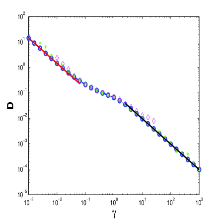
Figure 1: Diffusion coefficient as a function of the friction coefficient for the cosine potential. Dash-dot line and circles: $D$ obtained from the numerical solution of the Poisson equation, formula (4.4); stars: $D$ obtained from the the calculation of the jump length distribution and the hopping rate, formula (1.2);diamonds: results from Monte Carlo simulations, formula (1.3);solid lines, analytical approximation for $\gamma\ll 1,\;\gamma\gg 1$, equations (3.11) and (1.7).

We truncate (4.6) by taking into account the first $N+1$ terms of the Hermite expansion and the first $K+1$ terms of the Fourier expansion. This leads to a sparse linear system of $\left(N+1\right)\left(2K+1\right)$ equations and $\left(N+1\right)\left(2K+1\right)-1$ variables (note the absence of the term $\phi_{0\,0}$). This implies that one of the equations in (4.6) is linearly dependent on the others; to obtain a nonsingular system we remove the equation for $k=0$. In this way we obtain a nonsingular system of $s=\left(N+1\right)\left(2K+1\right)-1$ equations and unknowns. This system can be written in the form $\mathbf{Ax=b}$ with

$$x_{i}=\phi_{n\,k},\hskip 5.69046pti=\left\{\begin{array}[]{ll}k+K+1&n=0,k<0,\\ n\left(2K+1\right)+k+K&n=0,k>0$ or $n\neq 0\\ \end{array}\right.$$

and $\alpha_{i\,j}$ is the coefficient of $x_{j}$ in the $i^{th}$ equation, which is taken from equations (4.6) for values of $n$ and $k$

$$i=\left\{\begin{array}[]{ll}k+K+1&n=0,k<0\\ n\left(2K+1\right)+k+K&n=0,k>0$ or $n\neq 0\\ \end{array}\right.$$

The sparsity of this system implies that we can solve it very efficiently. In particular, we can calculate accurately the diffusion coefficient with a minimal computational cost, even for very small values of the friction constant $\gamma$.

To illustrate the efficiency of our numerical method, we calculate the diffusion coefficient for the cosine potential as a function of the dissipation $\gamma$, at a fixed temperature $\beta^{-1}=0.5$. We compare the results obtained through our numerical method with the approximate analytical expressions (1.7) and $~{}\eqref{e:risken}$, results from Monte Calro simulations using (1.3) and results obtained through numerical calculation of the hopping rate and the jump length distribution, equation (1.2). FOr the calculation of $\langle\ell^{2}\rangle$ and $\kappa$ we generate a long path (for every $\gamma$) of the Langevin dynamics using the Milstein scheme.

The results of the numerical simulations are presented in Figure 1. There agreement between the approximate analytical formulas and the calculation of the diffusion coefficient using the method described in this section are excellent. Our method is far superior in comparison to Monte Carlo simulations or the calculation of the mean square jump length and the hopping rate, since even for very small $\gamma$ the solution of a rather small linear system of equations is required. On the other hand, contrast, the path of integration over which we have to solve the Langevin equation in order to compute accurate statistics increases as $\gamma$ decreases and the calculation of $D$ using Monte Carlo becomes computationally expensive.

5 Conclusions

The problem of Brownian motion in a periodic potential in arbitrary dimensions was studied in this paper. Using multiscale techniques [25] we derived a formula for the effective diffusion tensor which is valid for all values of the friction coefficient and the temperature, and in arbitrary dimensions. We also showed the equivalence between our formula and the Green-Kubo formula. The calculation of the diffusion tensor using our approach requires the solution of a Poisson equation together with the calculation of the average of an appropriate function with respect to the canonical distribution. Furthermore, the overdamped and underdamped limits where studied and approximate analytical formulas for the diffusion coefficient in these two limits where obtained. In addition, a very efficient numerical method for the calculation of the diffusion coefficient was developed; this numerical method is based on the solution of the Poisson equation via a spectral method and it leads to the accurate and very efficient calculation of the diffusion coefficient even for very low values of the friction coefficient.

The approach developed in the paper for the study of the problem of diffusion in periodic potentials offers various advantages over other analytical and numerical methods. First, all the results reported in this paper can be justified rigorously and they can also lead to a rigorous analysis of the dependence of the diffusion tensor on the friction coefficient and on the temperature. A first step in this direction was taken in [12]. Second, our method enables us to study various distinguished limits of physical interest (such as the overdamped and underdamped limits) in a systematic fashion through asymptotic analysis of the Poisson equation. Third, it leads to an efficient numerical method for calculating the diffusion tensor through the numerical solution of the Poisson equation. The effectiveness of our method was shown in this paper for the one dimensional problem, for which analytical approximate formulas are can be derived. The method is also very efficient in two and three dimensions and can offer insight into the problem of Brownian motion in periodic potentials in higher dimensions. A thorough numerical investigation of the multidimensional problem will be presented elsewhere.

References

- [1] A. Barone and G. Paterno. Physics and Applications of the Josephson Effect. Wiley, New York, 1982.
- [2] O. M. Braun and R. Ferrando. Role of long jumps in surface diffusion. Phys. Rev. E, 65(6):061107, Jun 2002.
- [3] G. Caratti, R. Ferrando, R. Spadacini, and G.E. Tommei. An analytical approximation to the diffusion coefficient in overdamped multidimensional systems. Physica A, 246:115–131, 1997.
- [4] L. Y. Chen, M. R. Baldan, and S. C. Ying. Surface diffusion in the low-friction limit: Occurrence of long jumps. Phys. Rev. B, 54(12):8856–8861, Sep 1996.
- [5] W.T. Coffey, Y.P. Kalmykov, and J.T. Waldron. The Langevin equation. World Scientific, Singapore, 2004.
- [6] W. Dietrich, I. Peschel, and W.R. Schneider. Diffusion in periodic potentials. Z. Phys, 27:177–187, 1977.
- [7] K.D. Dobbs and D.J. Doren. Dynamics of molecular surface diffusion: Origins and consequences of long jumps. J. Chem. Phys., 97(5):3722–3735, 1992.
- [8] S.N. Ethier and T.G. Kurtz. Markov processes. Wiley Series in Probability and Mathematical Statistics: Probability and Mathematical Statistics. John Wiley & Sons Inc., New York, 1986.
- [9] M. Freidlin and M. Weber. A remark on random perturbations of the nonlinear pendulum. Ann. Appl. Probab., 9(3):611–628, 1999.
- [10] R. Gomer. Diffusion of adsorbates on metal surfaces. Rep. Prog. Phys., 53:917–1002, 1990.
- [11] R. Guantes, J.L. Vega, S. Miret-Artes, and E. Pollak. Kramers’ turnover theory for diffusion of Na atoms on a Cu(001) surface measured by He scattering. J. Chem. Phys, 119(5):2780–2791, 2003.
- [12] M. Hairer and G. A. Pavliotis. From ballistic to diffusive motion in periodic potentials. J. Stat. Phys., 131(1):175–202, 2008.
- [13] M. Hairer and G.A. Pavliotis. Periodic homogenization for hypoelliptic diffusions. J. Statist. Phys., 117(1-2):261–279, 2004.
- [14] P. Hanggi, P. Talkner, and M. Borkovec. Reaction-rate theory: fifty years after Kramers. Rev. Modern Phys., 62(2):251–341, 1990.
- [15] W. Horsthemke and R. Lefever. Noise-induced transitions, volume 15 of Springer Series in Synergetics. Springer-Verlag, Berlin, 1984. Theory and applications in physics, chemistry, and biology.
- [16] S. M. Kozlov. Effective diffusion for the Fokker-Planck equation. Mat. Zametki, 45(5):19–31, 124, 1989.
- [17] H. A. Kramers. Brownian motion in a field of force and the diffusion model of chemical reactions. Physica, 7:284–304, 1940.
- [18] A.M. Lacasta, J.M Sancho, A.H. Romero, I.M. Sokolov, and K. Lindenberg. From subdiffusion to superdiffusion of particles on solid surfaces. Phys. Rev. E, 70:051104, 2004.
- [19] S. Lifson and J.L. Jackson. On the self–diffusion of ions in polyelectrolytic solution. J. Chem. Phys, 36:2410, 1962.
- [20] B. Lindner, M. Kostur, and L. Schimansky-Geier. Optimal diffusive transport in a tilted periodic potential. Fluctuation and Noise Letters, 1(1):R25–R39, 2001.
- [21] S Miret-Artes and E. Pollak. The dynamics of activated surface diffusion. J. Phys: Condens. Matter, 17:S4133–S4150, 2005.
- [22] G.C. Papanicolaou and S. R. S. Varadhan. Ornstein-Uhlenbeck process in a random potential. Comm. Pure Appl. Math., 38(6):819–834, 1985.
- [23] G. A. Pavliotis and A. M. Stuart. Parameter estimation for multiscale diffusions. J. Stat. Phys., 127(4):741–781, 2007.
- [24] G.A. Pavliotis. A multiscale approach to Brownian motors. Phys. Lett. A, 344:331–345, 2005.
- [25] G.A. Pavliotis and A.M. Stuart. Multiscale methods, volume 53 of Texts in Applied Mathematics. Springer, New York, 2008. Averaging and homogenization.
- [26] R. L. R. L. Stratonovich. Topics in the theory of random noise. Vol. II. Revised English edition. Translated from the Russian by Richard A. Silverman. Gordon and Breach Science Publishers, New York, 1967.
- [27] P. Reimann. Brownian motors: noisy transport far from equilibrium. Phys. Rep., 361(2-4):57–265, 2002.
- [28] P. Reimann, C. Van den Broeck, H. Linke, P. Hanggi, J.M. Rubi, and A. Perez-Madrid. Giant acceleration of free diffusion by use of tilted periodic potentials. Phys. Rev. Let., 87(1):010602, 2001.
- [29] D. Revuz and M. Yor. Continuous martingales and Brownian motion, volume 293 of Grundlehren der Mathematischen Wissenschaften [Fundamental Principles of Mathematical Sciences]. Springer-Verlag, Berlin, third edition, 1999.
- [30] H. Risken. The Fokker-Planck equation, volume 18 of Springer Series in Synergetics. Springer-Verlag, Berlin, 1989.
- [31] J.M Sancho, A.M. Lacasta, K. Lindenberg, I.M. Sokolov, and A.H. Romero. Diffusion on a solid surface: anomalous is normal. Phys. Rev. Let, 92(25):250601, 2004.
- [32] M. Schunack, T. R. Linderoth, F. Rosei, E. Lægsgaard, I. Stensgaard, and F. Besenbacher. Long jumps in the surface diffusion of large molecules. Phys. Rev. Lett., 88(15):156102, Mar 2002.
- [33] Z. Schuss. Theory and applications of stochastic differential equations. John Wiley & Sons Inc., New York, 1980. Wiley Series in Probability and Statistics.
- [34] R. L. Stratonovich. Topics in the theory of random noise. Vol. I. Revised English edition. Translated from the Russian by Richard A. Silverman. Gordon and Breach Science Publishers, New York, 1963.
- [35] X-P Zhang and J-D Bao. Stochastic resonance in multidimensional periodic potential. Surf. Sci., 540:145–152, 2003.