Multiparticle Entanglement in the Lipkin-Meshkov-Glick Model

Abstract

The multiparticle entanglement in the Lipkin-Meshkov-Glick model has been discussed extensively in this paper. Measured by the global entanglement and its generalization, our calculation shows that the multiparticle entanglement can faithfully detect quantum phase transitions. For an antiferromagnetic case the multiparticle entanglement reaches the maximum at the transition point, whereas for ferromagnetic coupling, two different behaviors of multiparticle entanglement can be identified, dependent on the anisotropic parameter in the coupling.

I introduction

The exploration of the connection between statistical mechanics and quantum information has been extensive in recent years since the work preskill . Especially the research of entanglement in many-body systems has contributed to the comprehensive crossover between the two hot areas afov07 . Furthermore, the finding of integer or fractional quantum Hall effect in two-dimensional many-body systems imposes a challenge on the universal understanding of phase transitions, since the traditional theory for phase transition cannot incorporate these novel phenomena senthil . Recently the research of quantum entanglement in two-dimensional many-body systems provides the clear characterization for different quantum orders kitaev . These facts suggest that quantum entanglement would play a vital role in the understanding of many-body effects.

Bipartite entanglement was first studied, and focused on the connection to the criticality in spin-chain systemsoaff02 ; on02 . This interest comes from the fact that quantum phase transition is related to the construction of the long-range correlations in many-body systems. Hence it is a natural conjecture that quantum entanglement, as a depiction of the non-local correlation, could detect the appearance of long-range correlation. Great progress has been made for the block entanglement in many-body systems; the area law of block entanglement entropy has been generally constructed by the conformal field theory. Furthermore the violation of the area law has been identified as a reliable detection of quantum phase transitions in one-dimensional systems(see Ref. afov07 for a comprehensive review). However the situation becomes complex for high-dimensional systems: the violation of the area law in one-dimensional case when the system is critical, does not seem to hold in higher dimensionsafov07 . Even for pairwise entanglement in many-body systems the results are not satisfying . For example, the cutoff in the definition of concurrence may lead to unphysical results when one focuses on the connection of entanglement and phase transition in many-body systems yang .

The situation becomes more complex for multiparticle entanglement(ME) because of the absence of unified measurement for MEpv07 . However, it is a natural speculation that ME should play a more fundamental role than a bipartite one for the understanding of many-body effects with consideration of the universal interaction in many-body systems. Recently the discussions of ME in many-body systems have been given more attention because of the availability of some special entangled states, e.g., cluster states for one-way quantum computationbr01 , $n$-party Greenberger-Horne-Zeilinger(GHZ) state and $W$-statedvc00 . Although great effort has been devoted to the measurement of ME, the analytical or operational measurements exist only for some special casespv07 . The connection of quantum phase transition and ME has also been discussed extensively in wei05 ; cffp07 ; oliveira06 . However these discussions are mainly on the one-dimensional spin-1/2 $XY$ model, and the difficulty of calculating ME obstructs further exploration.

Recently, the global entanglement has been constructed for the quantification of ME by Meyer and Wallachmw02 , which possesses the virtues of the availability of analytical expression and operability. Moreover global entanglement is measurable experimentally since it is directly related to the mixedness of single partybrennen03 . Another important character of global entanglement is the monotonicity under local operations and classical communication (LOCC), if one notes that global entanglement is intimately related to the linear entropyhorodecki07 . Consequently, Oliveira and his collaborators improved this definition for measuring some special entangled states, e.g. $n$-party $W$ state or GHZ stateoliveira06 . Moreover the connection of the generalized global entanglement and quantum phase transition has also been explored in the one-dimensional spin-1/2 $XY$ model, in which entanglement reaches the maximum near to the transition pointoliveira06 .

It is interesting to note that the nearest neighbor coupling is beneficial to the formation of ME in the one-dimensional spin-1/2 $XY$ model. Since the particle correlation is short-ranged in this modelon02 , one should note that the maximum of global entanglement maybe come from the distribution of pairwise entanglementcffp07 ; facchi . Hence it is tempting to present a discussion about ME when the correlation is long range and the coupling is beyond the nearest neighbor case. Fortunately the Lipkin-Meshkov-Glick(LMG) modellmg provides us the benchmark for exploring this point since the collective interaction in this model. Then it is expected that ME would play a critical role.

Recently the entanglement in the LMG model has been extensively studied, such as concurrence vidal ; dv04 ; vmd04 , one-tanglevpa04 , entanglement entropyuv ; lp05 ; vdb07 and generalized entanglementsomma . The concurrence in the LMG model displays sensitivity to the appearance of quantum phase transitionvidal ; vmd04 , except for some special casesvmd04 . A possible explanation of this discrepancy is that the trace operation performed in the calculation of concurrence inevitably kills some correlations between spinsvmd04 . With respect to this point, Barnum and his collaborators constructed a subsystem-independent measure of entanglement, based on a distinguished subspace of observables for the systembkosv04 . The named generalized entanglement introduced by Barnum, et.al. has also been discussed in the LMG model, which displayed the ability of detecting the phase transitionssomma . Moreover the authors show the equivalency between generalized entanglement and the global entanglement defined by Meyer and Wallachmw02 . However, as shown in somma , it is indispensable for the construction of the distinguished subspace of observables to obtain the knowledge of the ground state in many-body systems, that in most cases is very difficult. The research of entanglement entropy in the LMG model shows that the entropy was divergent under thermodynamic limit near the phase transition point, and moreover shows a discontinuity at the critical point for the isotropic coupling casevdb07 .

The generalized global entanglement (gGE), defined by Oliveira, et. al.oliveira06 , is a generalization of the global entanglement (GE). With respect to the equivalence between Barnum’s generalized entanglement and GE, gGE provides a universal characterization of ME in many-body systems. Hence, it is interesting to present a comprehensive research of gGE and GE in the LMG model. Our discussion also presents detailed research for antiferromagnetic coupling and some interesting results can be obtained, which is rarely touched on in the previous works. I should point out that the goal for this paper focuses on the connection between ME, measured by gGE and GE respectively, and quantum phase transition in the LMG model. For this purpose, the paper is organized as following. In Sec.II the Hamiltonian is presented, and ground states are determined analytically. The phase diagram will be identified by introducing the proper parameter. In Sec.III the analytical expressions for gGE and GE are presented. Based on these formulas the multiparticle entanglements for ferro-magnetic and antiferro-magnetic couplings are discussed respectively. The conclusions and discussions are given in Sec. IV.

II Hamiltonian and ground state

The LMG model describes a set of spin-half particles coupled to all others with an interaction independent of the position and the nature of the elements. The Hamiltonian can be written as

$$H=-\frac{\lambda}{N}(S^{2}_{x}+\gamma S^{2}_{y})-h_{z}S_{z},$$ (1)

in which $S_{\alpha}=\sum_{i=1}^{N}\sigma^{i}_{\alpha}/2(\alpha=x,y,z)$ and the $\sigma_{\alpha}$ is the Pauli operator, and $N$ is the total particle number in this system. The prefactor $1/N$ is essential to ensure the convergence of the free energy per spin in the thermodynamic limit. Anti-ferromagnetic or ferromagnetic interaction can be obtained dependent on $\lambda<0$ or not($\lambda\neq 0$). The Hamiltonian preserves the total spin and does not couple the state having spin pointing in the direction perpendicular to the field, i.e.

$$[H,\textbf{S}^{2}]=0,[H,\prod_{i=1}^{N}\sigma_{z}^{i}]=0.$$ (2)

For isotropic coupling $\gamma=1$, $[H,S_{z}]=0$ and the spectrum of Eq.(1) can be determined exactly. However for $\gamma\neq 1$, the spectrum can be determined in principle by Bethe-type equationsplo and the analytical expressions are difficult to obtain.

A distinguished character of Eq. (1) is the collective interaction, which is the same for any particle and independent of the space configuration of the system. Because of long-range correlation between particles, the mean-field analysis is adaptive for this modelbotet . The research of phase transition in the LMG model has shown that there is a second-order transition at $h=h_{z}/|\lambda|=1$ for the ferromagnetic case and a first-order one at $h=0$ for the antiferromagnetic casebotet ; vidal .

A proper parameter for characterizing the phase diagram is the total spin in the direction $z$ for the ground state. For ferromagnetic coupling, one has

$$1-2\langle S_{z}\rangle/N=\begin{cases}0,&h>1\\ 1-h,&h\in[0,1),\end{cases}$$ (3)

which corresponds to the disorder-order transition, and obviously the point $h=1$ is a second-order phase transition point. This phase transition could be attributed to the disappearance of the energy gap; at the symmetric phase $h>1$ the energy gap above the ground state is finite, whereas at the broken phase $0\leq h<1$ the energy gap vanishes under thermodynamic limitdv04 . For antiferromagnetic coupling,

$$2\langle S_{z}\rangle/N=\begin{cases}1,&h>0\\ -1,&h<0;\end{cases}$$ (4)

Obviously there is a first-order phase transition at the point $h=0$. For this case the energy gap above ground state vanishes only at the transition point $h=0$ under thermodynamic limit, and no level crossing happens when $h\neq 0$vmd04 .

The ground state for $\gamma\neq 1$ can be determined analytically with the help of Holstein-Primakoff(HP) transformation and low-energy approximationdv04 . In Ref. cui06 , the ground state has been obtained with the consideration of the finite number effect. The general expression reads

$$|g\rangle = \frac{1}{c}\sum_{n=0}^{[N/2]}(-1)^{n}\sqrt{\frac{(2n-1)!!}{2n!!}}\tanh^{n}x|2n\rangle$$

$$c^{2} = \sum_{n=0}^{[N/2]}(-1)^{n}\frac{(2n-1)!!}{2n!!}\tanh^{2n}x$$ (5)

in which $|2n\rangle$ is the Fock state of the boson operator introduced by Holstein-Primakoff transformation and $[N/2]$ denotes the integer part not more than $N/2$. One should note that the determination of the ground state Eq. (II) is based on HP transformation, which preserves the symmetry Eq. (2), and the following discussion is heavily based on this ground state. Dependent on the style of interaction, $\tanh\_x$ has different expressions. For ferromagnetic case $\lambda>0$, it satisfies the relationvidal

$$\tanh 2x=\begin{cases}-\frac{1-\gamma}{2h-1-\gamma},&h>1\\ -\frac{h^{2}-\gamma}{2-h^{2}-\gamma},&0\leq h<1\end{cases}.$$ (6)

For antiferromagnetic coupling $\lambda<0$, it is determined by

$$\tanh\_2x=\frac{1-\gamma}{1+\gamma+2|h|}.$$ (7)

For isotropic case $\gamma=1$, the calculation is exact. The ground state can be formulated generally as $|g\rangle=|S=\frac{N}{2},S_{z}=M\rangle$. For ferromagnetic coupling,

$$M=\begin{cases}I[hN/2],&0\leq h<1\\ \frac{N}{2},&h\geq 1.\end{cases}$$ (8)

in which $I[n]$ expresses the integer not more than $n$. For antiferromagnetic coupling ,

$$M=\begin{cases}\frac{N}{2},&h>0\\ -\frac{N}{2},&h<0.\end{cases}$$ (9)

III Multiparticle Entanglement

Recently, Meyer and Wallach have constructed the global entanglement for measuring ME in spin systems. The main procedure is to first measure the entanglement between any party and the others, and then calculate the average of all possible bipartitionmw02 . Although the criticism that it is not a genuine ME measure because of the intimate connection to bipartite entanglement horodecki07 , it has been proven that the global entanglement is operational and more importantly, monotonic under LOCC. A simplified expressions for global entanglement is provided by Brennen brennen03

$$Q(|\phi\rangle)=2(1-\frac{1}{N}\sum_{k=0}^{N-1}\text{Tr}[\rho_{k}^{2}]).$$ (10)

For the LMG model, one can obtain $Q(|g\rangle)=2(1-\text{Tr}\rho_{1}^{2})$, in which $\rho_{1}$ stands for the single-particle reduced density operator. Furthermore, Oliveira and his collaborators have improved this definition in order that it can measure some special entangle states, e.g. $\otimes_{n}|EPR\rangle_{n}$ or $n$-party GHZ state. The main procedure is to measure the entanglement between any two parties and the others, and then average all possible bipartitionoliveira06 . In the LMG model, for the symmetry of particle permutation, the generalized global entanglement can be written as

$$E_{g}=\frac{4}{3}(1-\text{Tr}[\rho^{2}_{2}]).$$ (11)

in which $\rho_{2}$ denotes the reduced density operator for any two particles. $\rho_{1},\rho_{2}$ can be determined through the correlation functionswm02

$$\langle\sigma_{\alpha}\rangle = \frac{2}{N}\langle S_{\alpha}\rangle,$$

$$\langle\sigma_{1\alpha}\sigma_{2\alpha}\rangle = \frac{4\langle S^{2}_{\alpha}\rangle-N}{N(N-1)}$$

$$\langle\sigma_{1\alpha}\sigma_{2\beta}\rangle = \frac{2\langle[S_{\alpha},S_{\beta}]_{+}\rangle-N}{N(N-1)}(\alpha\neq\beta)$$ (12)

in which $\alpha,\beta=x,y,z$.

With respect to the symmetry Eq. (2) and the ground state Eq. (II), one can obtain GE and gGE respectively

$$Q(|g\rangle)=1-\langle\sigma_{z}\rangle^{2}$$

$$E_{g}=1-\frac{1}{3}(2\langle\sigma_{z}\rangle^{2}+\langle\sigma_{1x}\sigma_{2x}\rangle^{2}+\langle\sigma_{1y}\sigma_{2y}\rangle^{2}+\langle\sigma_{1z}\sigma_{2z}\rangle^{2}).$$ (13)

Based on Eqs. (II) and (III), ME in the LMG model can be decided analytically, and some interesting properties can be found. The discussion below is divided into two cases: one focuses on the anisotropic coupling, and the other is for isotropic coupling for which the exact results can be obtained.

III.1 anisotropic coupling

The analytical results can be obtained under large $N$ limit with the hypothesis that the excitation would only happen for the low energy statesvidal . Based on Eqs. (II) and (III), one obtains

$$\langle\sigma_{z}\rangle = 1-\frac{4}{Nc^{2}}\sum_{n=0}^{[N/2]}nc_{2n}^{2}$$

$$\langle\sigma_{1x}\sigma_{2x}\rangle = \frac{2}{N(N-1)c^{2}}\sum_{n=0}^{[N/2]}[\sqrt{(N-2n+2)(N-2n+1)2n(2n-1)}c_{2n-2}c_{2n}+2n(N-2n)c^{2}_{2n}]$$

$$\langle\sigma_{1y}\sigma_{2y}\rangle = \frac{-2}{N(N-1)c^{2}}\sum_{n=0}^{[N/2]}[\sqrt{(N-2n+2)(N-2n+1)2n(2n-1)}c_{2n-2}c_{2n}-2n(N-2n)c^{2}_{2n}]$$

$$\langle\sigma_{1z}\sigma_{2z}\rangle = 1-\frac{4}{N(N-1)c^{2}}\sum_{n=0}^{[N/2]}2n(n-2n)c^{2}_{2n}$$ (14)

in which $c_{2n}=(-1)^{n}\sqrt{\frac{(2n-1)!!}{2n!!}}\tanh^{n}\_x$ and $\tanh x$ is decided by Eqs.(6) and (7). From Eq. (III), ME can be determined analytically.

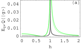
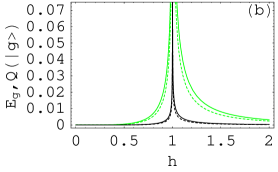
Figure 1: (Color online) The multiparticle entanglement for ferromagnetic coupling, measured by gGE (denoted by $E_{g}$ and solid lines) and GE (denoted by $Q(|g\rangle)$ and dashed lines) vs the rescaled magnetic field $h$. We have chosen $\gamma=0.5$(a) and $\gamma=0$(b) for this plot. The green and black solid lines correspond to $N=50,500$ respectively.

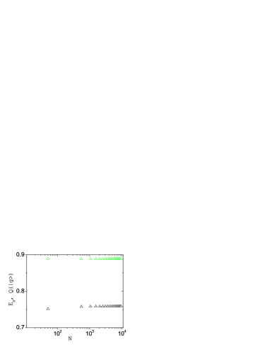
Figure 2: (Color online) $E_{g}$ (black triangles) and $Q(|g\rangle)$ (green triangles) for ferromagnetic coupling vs. the particle number $N$ at the phase transition point $h=1$. One should note that $\tanh 2x$ for any $\gamma\in[0,1)$ is identical in this case.

-Ferromagnetic case- gGE and GE have both been plotted for different $\gamma$ in Fig.1. It is obvious that ME reaches the maximum closed to phase transition point $h=1$ and the slope of curves tends to be infinite. In recent papersoliveira06 , the authors have shown that the singularity of gGE is directly connected to the degeneracy of the ground-state energy at the phase transition point. Since the energy gap above ground state vanishes at critical point $h=1$, the singularity of GE and gGE can be attributed to the degeneracy of ground-state energy, and could be used as a reliable detector for the phase transition in this case. Furthermore the finite-size scaling at the phase transition point $h=1$ displays the non-sensitivity both of gGE and GE to the particle number $N$, as shown in Fig.2.

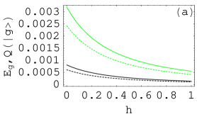
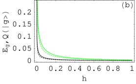
Figure 3: (Color online) $E_{g}$ (solid lines) and $Q(|g\rangle)$ (dashed lines) for antiferromagnetic coupling vs. the rescaled magnetic field $h$. The parameter $\gamma=0.5$(a) and $\gamma=0$(b) have been chosen for this plot. Since the system is invariant under the changing of $h\leftrightarrow-h$, these plottings are only for $h\geq 0$ with N=50 (green lines) and N=200 (black lines) respectively.

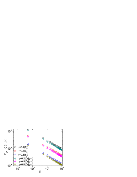
Figure 4: (Color online) $E_{g}$ and $Q(|g\rangle)$ for antiferromagnetic coupling vs. the particle number $N$ at first-order phase transition point $h=0$. We have choosen three representative values of $\gamma$ for this plot.

-Antiferromagnetic case- The situation is intricate. We have plotted GE and gGE vs. $h$ by choosing $\gamma=0$ (a) and $\gamma=1/2$ (b) respectively, in Fig.3. Since there is a first-order quantum phase transition, the figures show that GE and gGE both are maximum at transition point $h=0$. However a further calculation shows two different behaviors for ME; For $\gamma\in(0,1)$ GE and gGE show a cusp at phase transition point $h=0$, which means that the first derivation of gGE and GE with respect to $h$ is discontinued but finite at $h=0$. Since the degeneracy of ground-state energy happens only at $h=0$, this discontinuity of gGE and GE is attributed to the degeneracy of ground-state energy, whereas for $\gamma=0$, the figure shows that gGE and GE both have a drastic increase closed to the phase transition point, and the first derivations of gGE and GE with $h$ tend to be divergent. Furthermore our calculation shows that with the increasing of particle number, gGE and GE decrease for $\gamma\in(0,1)$ at the transition point, as shown in Fig. 4. Moreover, GE and gGE have similar behaviors and the difference between them is slight.

III.2 isotropic coupling

When $\gamma=1$, the exact results can be obtained. With respect to Eqs. (8), (9) and (III), one has in this case

$$E_{g} = 1-\frac{8M^{2}}{3N^{2}}-\frac{2(4M^{2}-N)^{2}+(4M^{2}-N^{2})^{2}}{6N^{2}(N-1)^{2}}$$

$$Q(|g\rangle) = 1-(\frac{2M}{N})^{2}.$$ (15)

Figure 5: $E_{g}$ (solid line) and $Q(|g\rangle)$ (dashed line) vs $h$ for isotropic ferromagnetic coupling with $N\rightarrow\infty$.

-Ferromagnetic case- With respect to Eqs. (8) and (III.2), both gGE and GE are zero for $h\geq 1$, independent of the particle number $N$ since the ground state is a direct-product state of $N$ particles with the same spin orientation from Eq. (8). As shown in Fig. 5, gGE and GE both are continued under thermodynamic limit at the phase transition $h=1$. This behavior is different from the conclusion made in Refs. lp05 ; vdb07 ; dv04 , in which entanglement entropy and concurrence both are discontinued at $h=1$ under thermodynamic limit. The main reason for this discrepancy is stated below. One notes that Eqs.(III.2) are a function of $M/N$. It is obvious from Eq. (8) that $M/N$ is continuous at the transition point $h=1$ under thermodynamic limit. Hence, it is not strange that gGE and GE are also continuous. Comparably the concurrence in dv04 is redefined by adding a prefactor $N-1$ to keep finite under thermodynamic limit. Similarly for the calculation of entanglement entropy, all possible bipartition has to be considered in the calculation to keep the entropy finite under thermodynamic limitlp05 , which I point out plays the same function of the prefactor $N-1$ for the calculation of concurrence. Under the thermodynamic limit, the prefactor would play a nontrivial role. Since the calculation for entanglement has been implemented respectively in different regions because of Eq. (8), the difference, which should disappear under thermodynamic limit, may become finite because of this prefactor. While, since our definition of ground state Eq.(II) has naturally considered the finite-number effect and GE and gGE are the functions of the correlations, one does not need this prefactor to keep the measurements of entanglement finite under thermodynamic limit. Together with respect that the equivalency between generalized entanglement and GE have been provedsomma , the measure gGE may also has the great virtue of independence on the concept of subsystem.

-Antiferromagnetic case- With respect to Eqs. (9) and (III.2), gGE and GE both vanish independently on $N$. Since the states for $M=\pm N/2$ are degenerate at phase transition point $h=0$, the ground state is undoubtedly the superposition of states $|N/2,N/2\rangle$ and $|N/2,-N/2\rangle$, written on the basis of $\{S^{2},S_{z}\}$, with equal weight,

$$|g\rangle=\frac{1}{\sqrt{2}}(|N/2,N/2\rangle+|N/2,-N/2\rangle).$$ (16)

Then in this case, a genuine maximally multiparticle entangled state, so called n-party GHZ statedvc00 , can be obtained at the point $h=0$ for a finite particle number, and under thermodynamic limit, it corresponds to the celebrated ( Schrödinger cat ) macroscopic quantum superposition state. Obviously, the measurement of entanglement is discontinued at $h=0$, where a first-order phase transition happens under thermodynamic limitfootnote1 .

IV discussions and conclusions

Some comments and discussions should be presented. In this paper an extensive discussion of multiparticle entanglement, measured by GE mw02 and gGE oliveira06 , is presented in the Lipkin-Meshkov-Glick model. Our discussion focuses on two different situations: for ferromagnetic coupling $\lambda>0$, when the anisotropic parameter $0<\gamma<1$ gGE and GE both reach the maximum at the second-order phase transition point $h=1$, as shown in Figs. 1. Moreover they are nonsensitive to the variation of particle number $N$, as shown in Fig.2. Whereas for the isotropic case $\gamma=1$ gGE and GE are zero at the phase transition point, shown in Fig. 5.

Another important situation is the appearance of antiferromagnetic coupling $\lambda<0$, for which there is a first-order phase transition at transition point $h=0$. gGE and GE both are calculated, as shown in Fig. 3. It is interesting that some different behaviors can be found in this case; one is that gGE and GE have a cusp at phase transition point when $\gamma\in(0,1)$, which means that the first derivation of gGE and GE with external magnetic field is discontinued but finite at $h=0$, shown in Fig. 3(a). Another case happens when $\gamma=0$, in which both gGE and GE have a drastic changing closed to $h=0$, shown in Fig. 3(b). Moreover our calculations show that gGE and GE for $\gamma\in(0,1)$ decrease with the increment of $N$ as shown in Fig.4, whereas for $\gamma=0$ they are non-sensitive to the particle number $N$. It is more interesting for the isotropic case that the entanglement is vanishing for $h\neq 0$ and has a sudden changing at $h=0$, where a genuine maximally multiparticle entanglement state, $n$-party GHZ state for finite particle number, can be obtained. With connection of a scheme of the realization of the LMG model in optical cavity QEDmp07 , this result provides a powerful method to create ME experimentally.

It was naturally expected that ME should be maximum at the phase transition point since the correlation between particles would be long-range because of the appearance of critical quantum fluctuation at the phase transition point. However an exceptional case appears in our discussion, which happens for ferromagnetic and isotropic coupling. In my own opinion, a reason for the difficulty in constructing the connection between entanglement and quantum phase transition is that the up-to-date measurements for entanglement are generally a nonlinear function of correlation functions in many-body systems. Hence the singularity of correlation functions may be canceledfootnote2 . As a concrete illustration one notes that for antiferromagnetic coupling, $M$ has a discontinued change at $h=0$ for $\gamma=1$, as shown in Eq.(9). However from Eq.(III.2) it is obvious that the discontinuity of $M$ for $h>0$ and $h<0$ has no effect on ME since gGE and GE are the functions of $M^{2}$.

Regardless of this defect, some interesting information can be obtained from the research of ME. An interesting speculation from our discussion is that the different finite-size scales may show the different state structures for the entanglement at the phase transition point. As shown previously in Ref. oliveira06 , with the increment of particle number the measures for entanglement for some states are decreasing, whereas for other states tend to be steady values. Since the increment of particle number, or more generally the degree of freedom, means the stronger correlation between the particles in many-body systems, one can conclude that some entangled states are immune to the effect imposed by the increment of correlation between particles, whereas others are sensitive to the changing of correlation. With respect to the pursuit of decoherence-free spacedfs , our discussion may provide some useful information.

With connection to the researches of the bipartite entanglement in many-body systems, one could note that it is difficult to construct a universal classification of phase transition based on the entanglement and its derivation. The main obstacle, in my own opinion, is the absence of physical definition of entanglement, i.e., how and what to define an ”entanglement operator”. Since quantum entanglement is an important physical resource and can be measured experimentally, I believe in the existence of this operator. Fortunately a few works have attributed to this directionsomma ; cv06 . I hope our discussion will help in the understanding of entanglement in many-body systems.

Acknowledgement The author acknowledges the support of Special Foundation of Theoretical Physics of NSF in China, Grant No. 10747159.

References

- (1) J. Preskill, J. Mod. Opt. 47, 127 (2000).
- (2) L. Amico, R. Fazio, A. Osterloh, V. Vedral, submitted to Rev. Mod. Phys. and available at e-print arXiv: quant-ph/0703044(2007).
- (3) T. Senthil, Proceedings of conference on ‘Recent Progress in Many-Body Theories’, Santa Fe, New Mexico (USA), Aug 23-27 (2004), also availible at e-print arXiv: cond-mat/0411275 (2004).
- (4) A. Y. Kitaev, Annals of Physics 303, 2 (2003); R. Moessner and S. L. Sondhi, Phys. Rev. Lett. 86, 1881 (2001); M. Levin and X.-G. Wen, Phys. Rev. B 71, 045110 (2005); P. Fendley and E. Fradkin, Phys. Rev. B 72, 024412(2005); A. Yu Kitaev, J. Preskill, Phys. Rev. Lett. 96, 110404(2006); M.A. Levin, X-G Wen, Phys. Rev. Lett. 96, 110405(2006).
- (5) A. Osterloh, L. Amico, G. Falci, R. Fazio, Nature, 416, 608(2002)
- (6) T. J. Osborne, M. A. Nielsen, Phys. Rev. A 66, 032110(2002).
- (7) M. F. Yang, Phys. Rev. A 71, 030302(2005).
- (8) Martin B. Plenio, Shashank Virmani, Quantum Inf. Comp. 7, 1(2007).
- (9) H.J. Briegel, R. Raussendorf, Phys. Rev. Lett. 86, 910(2001).
- (10) W. DÜr, G. Vidal, J.I. Cirac, Phys. Rev. A 62, 062314(2000).
- (11) T-C Wei, D. Das, S. Mukhopadyay, S. Vishveshwara, P.M. Goldbart, Phys. Rev. A 71, 060305(2005); S.J. Gu, G.S. Tian, H.Q. Lin, New J. Phys 8, 61(2006).
- (12) G. Costantini1, P. Facchi, G. Florio, S. Pascazio, J. Phys. A: Math. Theor. 40, 8009(2007).
- (13) de Oliveira, T. R., G. Rigolin, and M. C. de Oliveira, Phys. Rev. A 73, 010305(2006); de Oliveira, T. R., G. Rigolin, M. C. de Oliveira, and E. Miranda, Phys. Rev. Lett. 97, 170401(2006).
- (14) D. A. Meyer and N. R. Wallach, J. Math. Phys. 43, 4273(2002).
- (15) G. K. Brennen, Quant. Inf. Comp. 3, 619 (2003).
- (16) R. Horodecki, P. Horodecki, M. Horodecki, K. Horodecki, arXiv: quant-ph/0702225(2007).
- (17) P. Facchi, G. Florio, S. Pascazio, Phys. Rev. A 74, 042331 (2006).
- (18) H. J. Lipkin, N. Meshkov, A. J. Glick, Nucl. Phys. 62, 188 (1965); 62, 199 (1965); 62, 211(1965).
- (19) J. Vidal. G. Palacios, R. Mosseri, Phys. Rev. A, 69 , 022107(2004); J. Vidal, Phys. Rev. A 73, 062318(2006).
- (20) S. Dusuel, J. Vidal, Phys. Rev. Lett. 93, 237204 (2004); Phys. Rev. B 71, 224420 (2005).
- (21) J. Vidal, R. Mosseri, J. Dukelsky, Phys. Rev. A 69, 054101(2004).
- (22) J. Vidal, G. Palacios, C. Aslangul, Phys. Rev. A 70, 062304 (2004)
- (23) R. G. Unanyan, C. Ionescu, M. Fleischhauer, Phys. Rev. A 72, 022326 (2005).
- (24) J. I. Latorre, R. Orus, E. Rico, J. Vidal, Phys. Rev. A, 71, 064101 (2005);V. Popkov, M. Salerno, Phys. Rev. A 71, 012301(2005).
- (25) J. Vidal, S. Dusuel, T. Barthel, J. Stat. Mech. P01015(2007).
- (26) R. Somma, G. Ortiz, H. Barnum, E. Knill, L. Viodal, Phys. Rev. A 70, 042311 (2004).
- (27) H. Barnum, E. Knill, G. Ortiz, R. Somma, L. Viola, Phys. Rev. Lett. 92, 107902(2004).
- (28) F. Pan, J.P. Draayer, Phys. Lett. B 451, 1(1999); J. Links, H-Q. Zhou, R.H. McKenzie, M.D. Gould, J. Phys. A 36, R63(2003); G. Ortiz, R. Somma, J. Dukelsky, S. Rombouts, Nucl. Phys. B 707, 421(2005).
- (29) R. Botet, R. Jullien. P. Pfeuty, Phys. Rev. Lett. 49, 478 (1982); R. Botet, R. Jullien, Phys. Rev. B 28, 3955 (1983).
- (30) H.T. Cui, K. Li, X.X. Yi, Phys. Lett. A 360, 243(2006).
- (31) Xiaoguang Wang, K. Mølmer, Eur. Phys. J. D 18, 385(2002).
- (32) Eq. III.2 is obviously failed to measure the n-party GHZ state since its dependence on and the discontinuity of has no effect on ME.
- (33) S. Morrison, A. S. Parkins, e-print arXiv: quant-phy/0711.2325(2007).
-
(34)
The continuity of function is defined as
First suppose that is a linear function of the subfunctions , i.e. in which is the coefficient. Without lost of generality any is supposed not to be the linear combination of the other . Then the continuity of requires
The conclusion above means that the continuity of is sufficient and necessary condition for the continuity of . With respect of nonlinear case, let consider the function for simplicity. From the definition of the continuity and suppose , it requires
The prefactor has a nontrivial effect; Even if , the condition of continuity may still be satisfied only if this prefactor vanishes and keeps finite. - (35) I. L. Chuang and Y. Yamamoto, Phys. Rev. Lett. 76, 4281 (1996); L.-M. Duan and G. C. Guo, Phys. Rev. Lett. 79, 1953 (1997)
- (36) Clare Hewitt-Horsman, Vlatko Vedral, Phys. Rev. A 76, 062319 (2007); New J. Phys 9, 135 (2007).