Formulations of the Einstein equations for numerical simulations

Abstract

We review recent efforts to re-formulate the Einstein equations for fully relativistic numerical simulations. The so-called numerical relativity is a promising research field matching with ongoing gravitational wave observations. In order to complete a long-term and accurate simulations of binary compact objects, people seek a robust set of equations against the violation of constraints. Many trials have revealed that mathematically equivalent sets of evolution equations show different numerical stability in free evolution schemes. In this article, we overview the efforts of the community, categorizing them into three directions: (1) modifications of the standard Arnowitt-Deser-Misner equations initiated by the Kyoto group (the so-called Baumgarte-Shapiro-Shibata-Nakamura equations), (2) rewriting the evolution equations in a hyperbolic form, and (3) construction of an “asymptotically constrained” system. We then introduce our series of works that tries to explain these evolution behaviors in a unified way using eigenvalue analysis of the constraint propagation equations. The modifications of (or adjustments to) the evolution equations change the character of constraint propagation, and several particular adjustments using constraints are expected to damp the constraint-violating modes. We show several set of adjusted ADM/BSSN equations, together with their numerical demonstrations.

I Introduction

I.1 Overview

The theory of general relativity describes the nature of the strong gravitational field. The Einstein equation predicts quite unexpected phenomena such as gravitational collapse, gravitational waves, the expanding universe and so on, which are all attractive not only for researchers but also for the public. The Einstein equation consists of 10 partial differential equations (elliptic and hyperbolic) for 10 metric components, and it is not easy to solve them for any particular situation. Over the decades, people have tried to study the general-relativistic world by finding its exact solutions, by developing approximation methods, or by simplifying the situations. While “The Exact Solution” book exactsolution says there were more than 4000 publications on exact solutions between 1980 and 2000, direct numerical integration of the Einstein equations can be said to be the most robust way to study the strong gravitational field. This research field is often called “numerical relativity”.

With the purpose of the predictions of precise gravitational waveforms from coalescences of the binary neutron-stars and/or black-holes, numerical relativity has been developed for the past three decades. The difficulty of numerical integrations of the Einstein equations arises from its mathematical complexity of the equations, physical difficulty of singularity treatments, and from high-level requirements for computational skills and technology.

In 2005-2006, several groups independently announced that the simulations of the inspiral black-hole binary merger are available Pretorius ; Goddard ; UTB ; LSU ; PennState2006 . There are many implements for their successes, such as gauge conditions, coordinate selections, boundary treatments, singularity treatments, numerical discretization, and mesh refinements, together with the re-formulation of the Einstein equations which we will discuss here. More general and recent introductions to numerical relativity are available, e.g. by Baumgarte-Shapiro (2003) reviewBS , Alcubierre (2004) reviewAlcubierre , Pretorius (2007) reviewPretorius , and Bruegmann (2008) reviewBruegmann2008 .

The purpose of this article is to review the formulation problem in numerical relativity. This is one of the essential issues to achieve the long-term stable and accurate simulations of binary compact objects. Mathematically equivalent sets of evolution equations show different numerical stability in free evolution schemes. This had been the mystery for long time between the relativists, and many proposals and trials were reported. After we review the problem from such a historical viewpoint, we will explain our systematic understanding using the constraint propagation equations; the evolution equations of the constraints which is supposed to be satisfied all through the time evolutions.

The most numerical relativity groups today uses the so-called BSSN (Baumgarte-Shapiro-Shibata-Nakamura) equations, that is one of the modified form of the ADM (Arnowitt-Deser-Misner) equations. We try to explain why these differences appear and also predict that more robust sets of equations exist together with actual numerical demonstrations.

I.2 Formulation Problem in Numerical Relativity

There are several different approaches to simulating the Einstein equations. Among them the most robust way, that we target in this article, is to apply 3+1 (space + time) decomposition of space-time. This formulation was first given by Arnowitt, Deser and Misner (ADM) ADM (we call the original ADM system, hereafter) with the purpose of constructing a canonical formulation of the Einstein equations to seek the quantum nature of space-time. In late 70s, when the numerical relativity started, this ADM formulation was introduced by Smarr and York ADM-SmarrYork ; ADM-York in a slightly different notations which is taken as the standard formulation between numerical relativists (so that we call the standard ADM system, hereafter).

The ADM formulation divides the Einstein equations into the constraint equations and the evolution equations apparently, like the Maxwell equations. Since the set of ADM equations form a first-class system, if we solved two constraint equations, the Hamiltonian (or energy) constraint and the momentum constraint equations for the initial data, then the evolution equations theoretically guarantees the evolved data satisfy the constraint equations. This free-evolution approach is also the standard in numerical relativity. This is because solving the constraints (non-linear elliptic equations) is numerically expensive, and because the free-evolution allows us to monitor the accuracy of numerical evolution using the constraint equations.

Up to the middle 90s, the ADM numerical relativity appealed great successes. For example, the formation of naked singularity from collisionless particlesnakedsingularity shows the unknown behavior of the strong gravity; the discovery of the critical behavior for a black-hole formation criticalbehavior open-doors the understanding of phase-transition nature in general relativity; the black-hole horizon dynamics eventhorizon realized the theoretical predictions.

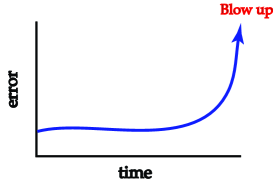
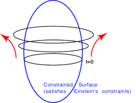
Figure 1: Origin of the problem for numerical relativists: Numerical evolutions depart from the constraint surface.

Nevertheless, when people try to make the long-term simulations such as coalescences of neutron-star binaries and/or black-hole binaries for calculating gravitational-wave form, numerical simulations were often interrupted by unexplained blow-ups (Figure 1). This was thought due to the lack of resolution, or inappropriate gauge choice, or the particular numerical scheme which was applied. However, with the accumulation of experiences, people have noticed the importance of the formulation of the evolution equations, since there are apparent differences in numerical stability although the equations are mathematically equivalent.

At this moment, there are three major ways to obtain longer time evolutions, which we describe in the next section. Of course, the ideas, procedures, and problems are mingled with each other. The purpose of this article is to review all three approaches and to introduce our idea to view them in a unified way. The author wrote a detail review of this topic in 2002 novabook , and the present article includes an update in brief style.

The word stability is used quite different ways in the community.

• We mean by numerical stability a numerical simulation which continues without any blow-ups and in which data remains on the constrained surface.

• Mathematical stability is defined in terms of the well-posedness in the theory of partial differential equations, such that the norm of the variables is bounded by the initial data. See eq. (28) and around.

• For numerical treatments, there is also another notion of stability, the stability of finite differencing schemes. This means that numerical errors (truncation, round-off, etc) are not growing by evolution. The evaluation is obtained using von Neumann’s analysis. Lax’s equivalence theorem says that if a numerical scheme is consistent (converging to the original equations in its continuum limit) and stable (no error growing), then the simulation represents the right (converging) solution. See Choptuik91 for the Einstein equations.

We follow the notations of that of MTWMTW . We use $\mu,\nu=0,\cdots,3$ and $i,j=1,\cdots,3$ as space-time indices. The unit $c=1$ is applied. The discussion is mostly to the vacuum space-time, but the inclusion of matter is straightforward.

II The standard way and the three other roads

II.1 Strategy 0: The ADM formulation

II.1.1 The original ADM formulation

The Arnowitt-Deser-Misner (ADM) formulationADM gave the fundamental idea of time evolution of space and time: such as foliations of 3-dimensional hypersurface (Figure 2).

The story begins by decomposing 4-dimensional space-time into 3 plus 1. The metric is expressed by

$$ds^{2} = g_{\mu\nu}dx^{\mu}dx^{\nu}$$ (1)

$$= -\alpha^{2}dt^{2}+\gamma_{ij}(dx^{i}+\beta^{i}dt)(dx^{j}+\beta^{j}dt),$$

where $\alpha$ and $\beta_{j}$ are defined as $\alpha\equiv 1/\sqrt{-g^{00}}$ and $\beta_{j}\equiv g_{0j},$ and called the lapse function and shift vector, respectively. The projection operator or the intrinsic 3-metric $g_{ij}$ is defined as $\gamma_{\mu\nu}=g_{\mu\nu}+n_{\mu}n_{\nu}$, where $n_{\mu}=(-\alpha,0,0,0)$ [and $n^{\mu}=g^{\mu\nu}n_{\nu}=(1/\alpha,-\beta^{i}/\alpha)$] is the unit normal vector of the spacelike hypersurface, $\Sigma$ (see Figure 2). By introducing the extrinsic curvature,

$$K_{ij} = -\frac{1}{2}\pounds_{n}\gamma_{ij},$$ (2)

and using the Gauss-Codacci relation, the Hamiltonian density of the Einstein equations can be written as

$${\cal H}_{GR}=\pi^{ij}\dot{\gamma}_{ij}-{\cal L},$$ (3)

where

$${\cal L}=\sqrt{-g}R=\alpha\sqrt{\gamma}[{}^{(3)\!}R-K^{2}+K_{ij}K^{ij}],$$ (4)

where $\pi^{ij}$ is the canonically conjugate momentum to $\gamma_{ij}$,

$$\pi^{ij}={\partial{\cal L}\over\partial\dot{\gamma}_{ij}}=-\sqrt{\gamma}(K^{ij}-K\gamma^{ij}),$$ (5)

omitting the boundary terms. The variation of ${\cal H}_{GR}$ with respect to $\alpha$ and $\beta_{i}$ yields the constraints, and the dynamical equations are given by $\dot{\gamma}_{ij}={\delta{\cal H}_{GR}\over\delta\pi^{ij}}$ and $\dot{\pi}^{ij}=-{\delta{\cal H}_{GR}\over\delta h_{ij}}$.

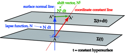
Figure 2: Concept of time evolution of space-time: foliations of 3-dimensional hypersurface. The lapse and shift functions are often denoted $\alpha$ or $N$, and $\beta^{i}$ or $N^{i}$, respectively.

II.1.2 The standard ADM formulation

In the version of Smarr and YorkADM-SmarrYork ; ADM-York , $K_{ij}$ was used as a fundamental variable instead of the conjugate momentum $\pi^{ij}$. The set of equation is summarized as follows:

$\Box$The Standard ADM formulation ADM-SmarrYork ; ADM-York
The fundamental dynamical variables are $(\gamma_{ij},K_{ij})$, the three-metric and extrinsic curvature. The three-hypersurface $\Sigma$ is foliated with gauge functions, ($\alpha,\beta^{i}$), the lapse and shift vector.

• The evolution equations:

  $${\partial_{t}}\gamma_{ij} = -2\alpha K_{ij}+D_{i}\beta_{j}+D_{j}\beta_{i},$$ (6)

  $${\partial_{t}}K_{ij} = \alpha~{}^{(3)\!}R_{ij}+\alpha KK_{ij}-2\alpha K_{ik}{K^{k}}_{j}-D_{i}D_{j}\alpha$$ (7)

  $$+(D_{i}\beta^{k})K_{kj}+(D_{j}\beta^{k})K_{ki}+\beta^{k}D_{k}K_{ij}$$

  where $K=K^{i}{}_{i}$, and $~{}^{(3)\!}R_{ij}$ and $D_{i}$ denote three-dimensional Ricci curvature, and a covariant derivative on the three-surface, respectively.

• Constraint equations:

  $${\cal H}^{ADM} := ~{}^{(3)\!}R+K^{2}-K_{ij}K^{ij}\approx 0,$$ (8)

  $${\cal M}^{ADM}_{i} := D_{j}K^{j}{}_{i}-D_{i}K\approx 0,$$ (9)

  where $~{}^{(3)\!}R=^{(3)\!}R^{i}{}_{i}$: these are called the Hamiltonian (or energy) and momentum constraint equations, respectively. $\qquad\Box$

The formulation has 12 first-order dynamical variables ($\gamma_{ij},K_{ij}$), with 4 freedom of gauge choice ($\alpha,\beta_{i}$) and with 4 constraint equations, (8) and (9). The rest freedom expresses 2 modes of gravitational waves.

We remark that there is one replacement in (7) using (8) in the process of conversion from the original ADM to the standard ADM equations. This is the key issue in the later discussion, and we shall be back this point in §III.2.

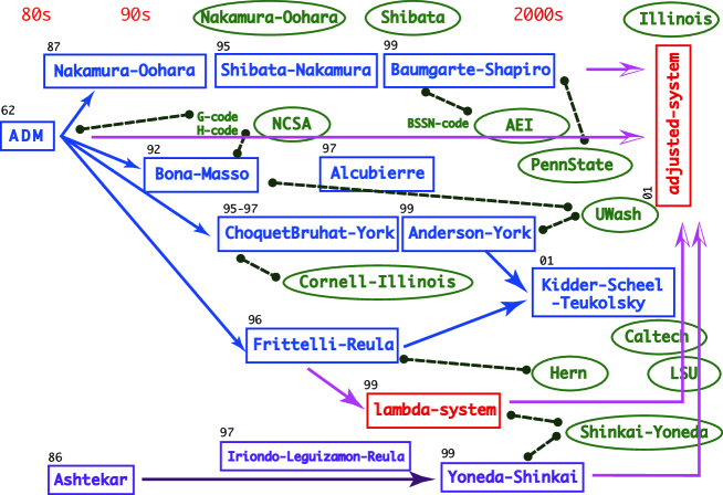
Figure 3: Chronological table of formulations and their numerical tests ($\sim$ 2001). Boxed ones are of proposals of formulation, circled ones are related numerical experiments. Please refer Table 1 in novabook for each references.

The constraint propagation equations, which are the time evolution equations of the Hamiltonian constraint (8) and the momentum constraints (9), can be written as follows:

$\Box$Constraint Propagations of the Standard ADM:

$$\partial_{t}{\cal H} = \beta^{j}(\partial_{j}{\cal H})+2\alpha K{\cal H}-2\alpha\gamma^{ij}(\partial_{i}{\cal M}_{j})$$ (10)

$$+\alpha(\partial_{l}\gamma_{mk})(2\gamma^{ml}\gamma^{kj}-\gamma^{mk}\gamma^{lj}){\cal M}_{j}$$

$$-4\gamma^{ij}(\partial_{j}\alpha){\cal M}_{i},$$

$$\partial_{t}{\cal M}_{i} = -(1/2)\alpha(\partial_{i}{\cal H})-(\partial_{i}\alpha){\cal H}+\beta^{j}(\partial_{j}{\cal M}_{i})+\alpha K{\cal M}_{i}$$ (11)

$$-\beta^{k}\gamma^{jl}(\partial_{i}\gamma_{lk}){\cal M}_{j}+(\partial_{i}\beta_{k})\gamma^{kj}{\cal M}_{j}.\qquad\Box$$

From these equations, we know that if the constraints are satisfied on the initial slice $\Sigma$, then the constraints are satisfied throughout evolution. The normal numerical scheme is to solve the elliptic constraints for preparing the initial data, and to apply the free evolution (solving only the evolution equations). The constraints are used to monitor the accuracy of simulations.

The ADM formulation was the standard formulation for numerical relativity up to the middle 90s. Numerous successful simulations were obtained for the problems of gravitational collapse, critical behavior, cosmology, and so on. However, stability problems have arisen for the simulations such as the gravitational radiation from compact binary coalescence, because the models require quite a long-term time evolution.

The origin of the problem was that the above statement in Italics is true in principle, but is not always true in numerical applications. A long history of trial and error began in the early 90s. From the next subsection we shall look back of them by summarizing “three strategies”. We then unify these three roads as “adjusted systems”, and as its by-product we show that the standard ADM equations has a constraint violating mode in its constraint propagation equations even for a single black-hole (Schwarzschild) spacetime adjADMsch . Figure 3 and 4 are chronological maps of the researches.

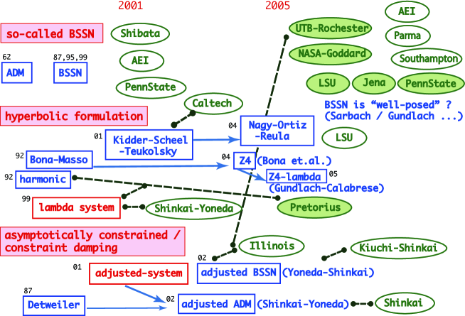
Figure 4: Chronological table of formulations and their numerical tests (2001 $\sim$). Boxed ones are of proposals of formulation, circled ones are related numerical experiments.

II.2 Strategy 1: Modified ADM formulation by Nakamura et al (The BSSN formulation)

Up to now, the most widely used formulation for large scale numerical simulations is a modified ADM system, which is now often cited as the Baumgarte-Shapiro-Shibata-Nakamura (BSSN) formulation. This re-formulation was first introduced by Nakamura et al. SN87 ; SN89 ; SN . The usefulness of this re-formulation was re-introduced by Baumgarte and Shapiro BS , then was confirmed by other groups to show a long-term stable numerical evolution potsdam9908 ; potsdam0003 .

II.2.1 Basic variables and equations

The widely used notationBS introduces the variables ($\varphi,\tilde{\gamma}_{ij}$,$K$,$\tilde{A}_{ij}$,$\tilde{\Gamma}^{i}$) instead of ($\gamma_{ij}$,$K_{ij}$), where

$$\varphi = {1\over 12}\log({\rm det}\gamma_{ij}),$$ (12)

$$\tilde{\gamma}_{ij} = e^{-4\varphi}\gamma_{ij},$$ (13)

$$K = \gamma^{ij}K_{ij},$$ (14)

$$\tilde{A}_{ij} = e^{-4\varphi}(K_{ij}-(1/3)\gamma_{ij}K),$$ (15)

$$\tilde{\Gamma}^{i} = \tilde{\Gamma}^{i}_{jk}\tilde{\gamma}^{jk}.$$ (16)

The new variable $\tilde{\Gamma}^{i}$ is introduced in order to calculate Ricci curvature more accurately. In BSSN formulation, Ricci curvature is not calculated as $R^{ADM}_{ij}=\partial_{k}\Gamma^{k}_{ij}-\partial_{i}\Gamma^{k}_{kj}+\Gamma^{l}_{ij}\Gamma^{k}_{lk}-\Gamma^{l}_{kj}\Gamma^{k}_{li},$ but as $R^{BSSN}_{ij}=R^{\varphi}_{ij}+\tilde{R}_{ij}$, where the first term includes the conformal factor $\varphi$ while the second term does not. These are approximately equivalent, but $R^{BSSN}_{ij}$ does have wave operator apparently in the flat background limit, so that we can expect more natural wave propagation behavior.

Additionally, the BSSN requires us to impose the conformal factor as $\tilde{\gamma}(:={\rm det}\tilde{\gamma}_{ij})=1,$ during evolution. This is a kind of definition, but can also be treated as a constraint.

$\Box$The BSSN formulation SN87 ; SN89 ; SN ; BS :
The fundamental dynamical variables are ($\varphi,\tilde{\gamma}_{ij}$,$K$,$\tilde{A}_{ij}$,$\tilde{\Gamma}^{i}$).
The three-hypersurface $\Sigma$ is foliated with gauge functions, ($\alpha,\beta^{i}$), the lapse and shift vector.

• The evolution equations:

  $$\partial_{t}^{B}\varphi = -(1/6)\alpha K+(1/6)\beta^{i}(\partial_{i}\varphi)+(\partial_{i}\beta^{i}),$$ (17)

  $$\partial_{t}^{B}\tilde{\gamma}_{ij} = -2\alpha\tilde{A}_{ij}+\tilde{\gamma}_{ik}(\partial_{j}\beta^{k})+\tilde{\gamma}_{jk}(\partial_{i}\beta^{k})$$ (18)

  $$-(2/3)\tilde{\gamma}_{ij}(\partial_{k}\beta^{k})+\beta^{k}(\partial_{k}\tilde{\gamma}_{ij}),$$

  $$\partial_{t}^{B}K = -D^{i}D_{i}\alpha+\alpha\tilde{A}_{ij}\tilde{A}^{ij}+(1/3)\alpha K^{2}+\beta^{i}(\partial_{i}K),$$ (19)

  $$\partial_{t}^{B}\tilde{A}_{ij} = -e^{-4\varphi}(D_{i}D_{j}\alpha)^{TF}+e^{-4\varphi}\alpha(R^{BSSN}_{ij})^{TF}$$ (20)

  $$+\alpha K\tilde{A}_{ij}-2\alpha\tilde{A}_{ik}\tilde{A}^{k}{}_{j}+(\partial_{i}\beta^{k})\tilde{A}_{kj}+(\partial_{j}\beta^{k})\tilde{A}_{ki}$$

  $$-(2/3)(\partial_{k}\beta^{k})\tilde{A}_{ij}+\beta^{k}(\partial_{k}\tilde{A}_{ij}),$$

  $$\partial_{t}^{B}\tilde{\Gamma}^{i} = -2(\partial_{j}\alpha)\tilde{A}^{ij}+2\alpha\big{(}\tilde{\Gamma}^{i}_{jk}\tilde{A}^{kj}-(2/3)\tilde{\gamma}^{ij}(\partial_{j}K)$$ (21)

  $$+6\tilde{A}^{ij}(\partial_{j}\varphi)\big{)}-\partial_{j}\big{(}\beta^{k}(\partial_{k}\tilde{\gamma}^{ij})-\tilde{\gamma}^{kj}(\partial_{k}\beta^{i})$$

  $$-\tilde{\gamma}^{ki}(\partial_{k}\beta^{j})+(2/3)\tilde{\gamma}^{ij}(\partial_{k}\beta^{k})\big{)}.$$

• Constraint equations:

  $${\cal H}^{BSSN} = R^{BSSN}+K^{2}-K_{ij}K^{ij},$$ (22)

  $${\cal M}^{BSSN}_{i} = {\cal M}^{ADM}_{i},$$ (23)

  $${\cal G}^{i} = \tilde{\Gamma}^{i}-\tilde{\gamma}^{jk}\tilde{\Gamma}^{i}_{jk},$$ (24)

  $${\cal A} = \tilde{A}_{ij}\tilde{\gamma}^{ij},$$ (25)

  $${\cal S} = \tilde{\gamma}-1.\qquad\Box$$ (26)

(22) and (23) are the Hamiltonian and momentum constraints (the “kinematic” constraints), while the latter three are “algebraic” constraints due to the requirements of BSSN variables.

II.2.2 Remarks, Pros and Cons

Why BSSN is better than the standard ADM? Together with numerical comparisons with the standard ADM casepotsdam0003 , this question has been studied by many groups using different approaches.

• Using numerical test evolutions, Alcubierre et al. potsdam9908 found that the essential improvement is in the process of replacing terms by the momentum constraints. They also pointed out that the eigenvalues of BSSN evolution equations have fewer “zero eigenvalues” than those of ADM, and they conjectured that the instability might be caused by these “zero eigenvalues”.

• MillerMiller reported that BSSN has a wider range of parameters that gives us stable evolutions in von Neumann’s stability analysis.

• An effort was made to understand the advantage of BSSN from the point of hyperbolization of the equations in its linearized limit potsdam9908 ; LSU-BSSN , or with a particular combination of slicing conditions plus auxiliary variablesHeyerSarbach . If we define the 2nd order symmetric hyperbolic form, then the principal part of BSSN can be one of themGundlach0406 .

As we discussed in adjBSSN , the stability of the BSSN formulation is due not only to the introductions of new variables, but also to the replacement of terms in the evolution equations using the constraints. Further, we can show several additional adjustments to the BSSN equations which give us more stable numerical simulations. We will devote §III for the fundamental idea.

The current binary black-hole simulations apply the BSSN formulations with several implementations. For example,

• Alcubierre et al. potsdam0003 reported that trace-out $A_{ij}$ technique at every time-step helps the stability.

• Campanelli et al. UTB reported that in their code $\tilde{\Gamma}^{i}$ is replaced by $-\partial_{j}\tilde{\gamma}^{ij}$ where it is not differentiated.

• Baker et al. Goddard modified $\tilde{\Gamma}^{i}$-equation (21) as suggested by Yo et al. YBS .

These technical tips are again explained using the constraint propagation analysis as we will come back in §III.3.1.

These studies provide sort of evidences regarding the advantage of BSSN, while it is also shown an example of an ill-posed solution in BSSN (as well in ADM) by Frittelli and Gomez FrittelliGomez . Recently, the popular combination, BSSN with Bona-Masso type slicing condition, is investigated in particular. Among then, Garfinkle et al. GGH0707 speculated that the reason of gauge shocks are missing in the current 3-dimensional black-hole simulations is simply because the lack of resolution.

II.3 Strategy 2: Hyperbolic re-formulations

II.3.1 Definitions, properties, mathematical backgrounds

The second effort to re-formulate the Einstein equations is to make the evolution equations reveal a first-order hyperbolic form explicitly. This is motivated by the expectation that the symmetric hyperbolic system has well-posed properties in its Cauchy treatment in many systems and also that the boundary treatment can be improved if we know the characteristic speed of the system.

$\Box$Hyperbolic formulations
We say that the system is a first-order (quasi-linear) partial differential equation system, if a certain set of (complex-valued) variables $u_{\alpha}$ $(\alpha=1,\cdots,n)$ forms

$$\partial_{t}u_{\alpha}={\cal M}^{l}{}^{\beta}{}_{\alpha}(u)\,\partial_{l}u_{\beta}+{\cal N}_{\alpha}(u),$$ (27)

where ${\cal M}$ (the characteristic matrix) and ${\cal N}$ are functions of $u$ but do not include any derivatives of $u$. Further we say the system is

• a weakly hyperbolic system, if all the eigenvalues of the characteristic matrix are real.

• a strongly hyperbolic system (or a diagonalizable / symmetrizable hyperbolic system), if the characteristic matrix is diagonalizable (has a complete set of eigenvectors) and has all real eigenvalues.

• a symmetric hyperbolic system, if the characteristic matrix is a Hermitian matrix. $\qquad\Box$

Writing the system in a hyperbolic form is a quite useful step in proving that the system is well-posed. The mathematical well-posedness of the system means ($1^{\circ}$) local existence (of at least one solution $u$), ($2^{\circ}$) uniqueness (i.e., at most solutions), and ($3^{\circ}$) stability (or continuous dependence of solutions $\{u\}$ on the Cauchy data) of the solutions. The resultant statement expresses the existence of the energy inequality on its norm,

$$||u(t)||\leq e^{\alpha\tau}||u(t=0)||,$$

$$\quad\mbox{\rm where~{}}0<\tau<t,\quad\alpha={\rm const.}$$ (28)

This indicates that the norm of $u(t)$ is bounded by a certain function and the initial norm. Remark that this mathematical bounds does not mean that the norm $u(t)$ decreases along the time evolution.

The inclusion relation of the hyperbolicities is,

symmetric hyperbolic $$\subset$$ strongly hyperbolic (29)

$$\subset \mbox{\rm weakly~{}hyperbolic}.$$

The Cauchy problem under weak hyperbolicity is not, in general, $C^{\infty}$ well-posed. At the strongly hyperbolic level, we can prove the finiteness of the energy norm if the characteristic matrix is independent of $u$ (cf Stewart ), that is one step definitely advanced over a weakly hyperbolic form. Similarly, the well-posedness of the symmetric hyperbolic is guaranteed if the characteristic matrix is independent of $u$, while if it depends on $u$ we have only limited proofs for the well-posedness.

From the point of numerical applications, to hyperbolize the evolution equations is quite attractive, not only for its mathematically well-posed features. The expected additional advantages are the following.

• It is well known that a certain flux conservative hyperbolic system is taken as an essential formulation in the computational Newtonian hydrodynamics when we control shock wave formations due to matter.

• The characteristic speed (eigenvalues of the principal matrix) is supposed to be the propagation speed of the information in that system. Therefore it is naturally imagined that these magnitudes are equivalent to the physical information speed of the model to be simulated.

• The existence of the characteristic speed of the system is expected to give us an improved treatment of the numerical boundary, and/or to give us a new well-defined Cauchy problem within a finite region (the so-called initial boundary value problem; IBVP).

These statements sound reasonable, but have not yet been generally confirmed in actual numerical simulations in general relativity.

II.3.2 Hyperbolic formulations of the Einstein equations

Most physical systems can be expressed as symmetric hyperbolic systems. In order to prove that the Einstein’s theory is a well-posed system, to hyperbolize the Einstein equations is a long-standing research area in mathematical relativity.

The standard ADM system does not form a first order hyperbolic system. This can be seen immediately from the fact that the ADM evolution equation (7) has Ricci curvature in RHS. This is also the common fact to the BSSN formulation.

So far, several first order hyperbolic systems of the Einstein equation have been proposed. In constructing hyperbolic systems, the essential procedures are (1^∘) to introduce new variables, normally the spatially derivatived metric, (2^∘) to adjust equations using constraints. Occasionally, (3^∘) to restrict the gauge conditions, and/or (4^∘) to rescale some variables. Due to process (1^∘), the number of fundamental dynamical variables is always larger than that of ADM.

Due to the limitation of space, we can only list several hyperbolic systems of the Einstein equations:

• The Bona-Massó formulation BM ; BMSS

• The Einstein-Ricci system CY9506071 ; CY9506072 / Einstein-Bianchi system CY9710041

• The Einstein-Christoffel system AY

• The Ashtekar formulation Ashtekar ; ysPRL

• The Frittelli-Reula formulation FR96 ; Stewart

• The Conformal Field equations FriedrichCFE

• The Bardeen-Buchman system BB

• The Kidder-Scheel-Teukolsky (KST) formulation KST

• The Alekseenko-Arnold system AA2003

• The general-covariant Z4 system Z4

• The Nagy-Ortiz-Reula (NOR) formulation NOR

• The Weyl system FriedrichWeyl ; FrauendienerVogel

Note that there is no apparent differences between the word ‘formulation’ and ‘system’ here.

II.3.3 Numerical tests

When we discuss hyperbolic systems in the context of numerical stability, the following questions should be considered:

• From the point of the set of evolution equations, does hyperbolization actually contribute to numerical accuracy and stability? Under what conditions/situations will the advantages of hyperbolic formulation be observed?

Unfortunately, we do not have conclusive answers to these questions, but many experiences are being accumulated. Several earlier numerical comparisons reported the stability of hyperbolic formulations BMSS ; cactus1 ; SBCSThyper ; SBCST98 . But we have to remember that this statement went against the standard ADM formulation.

These partial numerical successes encouraged the community to formulate various hyperbolic systems. However, several numerical experiments also indicate that this direction is not a complete success.

• Above earlier numerical successes were also terminated with blow-ups.

• If the gauge functions are evolved according to the hyperbolic equations, then their finite propagation speeds may cause pathological shock formations in simulations Alcubierre ; AM .

• There are no drastic differences in the evolution properties between hyperbolic systems (weakly, strongly and symmetric hyperbolicity) by systematic numerical studies by Hern HernPHD based on Frittelli-Reula formulation FR96 , and by the authors ronbun1 based on Ashtekar’s formulation Ashtekar ; ysPRL .

• Proposed symmetric hyperbolic systems were not always the best ones for numerical evolution. People are normally still required to re-formulate them for suitable evolution. Such efforts are seen in the applications of the Einstein-Ricci system SBCST98 , the Einstein-Christoffel system BB , and so on.

• If we can erase the non-principal part by suitable re-definition of variables (as is in the KST formulation)KST , then we can see the growth of energy norm (28) in numerical evolution as theoretically predicted LindblomScheel ; LSU-KST . We then see a certain differences in the long-term convergence features between weakly and strongly hyperbolic systems.

Of course, these statements only casted on a particular formulation, and therefore we have to be careful not to over-emphasize the results.

II.3.4 Remarks

In order to figure out the reasons for the above objections, it is worth stating the following cautions:

• Rigorous mathematical proofs of well-posedness of PDE are mostly for simple symmetric or strongly hyperbolic systems. If the matrix components or coefficients depend on dynamical variables (as in all any versions of hyperbolized Einstein equations), almost nothing was proved in more general situations.

• The statement of “stability” in the discussion of well-posedness refers to the bounded growth of the norm, (28), and does not indicate a decay of the norm in time evolution.

• The discussion of hyperbolicity only uses the characteristic part of the evolution equations, and ignores the rest.

We think the origin of confusion in the community results from over-expectation on the above issues. Mostly, point (c) is the biggest problem. The above numerical claims from Ashtekarronbun1 ; ronbun2 and Frittelli-Reula HernPHD formulations were mostly due to the contribution (or interposition) of non-principal parts in evolution. Regarding this issue, the KST formulation finally opens the door. KST’s “kinematic” parameters enable us to reduce the non-principal part, so that numerical experiments are hopefully expected to represent predicted evolution features from PDE theories. At this moment, the agreement between numerical behavior and theoretical prediction is not yet perfect but close LindblomScheel .

If further studies reveal the direct correspondences between theories and numerical results, then the direction of hyperbolization will remain as the essential approach in numerical relativity, and the related IBVP researches Stewart ; IBVP-FN ; IBVP-BS ; IBVP-KRSW ; IBVP-RRS will become a main research subject in the future. Meanwhile, it will be useful if we have an alternative procedure to predict stability including the effects of the non-principal parts of the equations. Our proposal of adjusted system in the next subsection may be one of them.

II.4 Strategy 3: Asymptotically constrained systems

The third strategy is to construct a robust system against the violation of constraints, such that the constraint surface is an attractor (Figure 5). The idea was first proposed as “$\lambda$-system” by Brodbeck et al. BFHR , and then developed in more general situations as “adjusted system” by the authors ronbun2 .

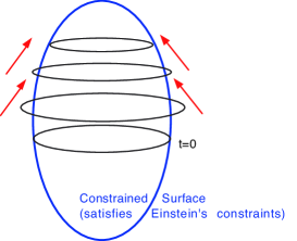
Figure 5: The idea of the “Asymptotically Constrained System”.

II.4.1 The “$\lambda$-system”

Brodbeck et al. BFHR proposed a system which has additional variables $\lambda$ that obey artificial dissipative equations. The variable $\lambda$s are supposed to indicate the violation of constraints and the target of the system is to get $\lambda=0$ as its attractor.

$\Box$The “$\lambda$-system” (Brodbeck et al.) BFHR :
For a symmetric hyperbolic system, add additional variables $\lambda$ and artificial force to reduce the violation of constraints. The procedure is as follows:

1. Prepare a symmetric hyperbolic evolution system

   $$\partial_{t}u=M\partial_{i}u+N$$ (30)

2. Introduce $\lambda$ as an indicator of violation of constraint which obeys dissipative eqs. of motion

   $$\partial_{t}\lambda=\alpha C-\beta\lambda,(\alpha\neq 0,\beta>0)$$ (31)

3. Take a set of $(u,\lambda)$ as dynamical variables

   $$\partial_{t}\left(\begin{matrix}u\\ \lambda\end{matrix}\right)\simeq\left(\begin{matrix}A&0\\ F&0\end{matrix}\right)\partial_{i}\left(\begin{matrix}u\\ \lambda\end{matrix}\right)$$ (32)

4. Modify evolution eqs so as to form a symmetric hyperbolic system

   $$\partial_{t}\left(\begin{matrix}u\\ \lambda\end{matrix}\right)=\left(\begin{matrix}A&\bar{F}\\ F&0\end{matrix}\right)\partial_{i}\left(\begin{matrix}u\\ \lambda\end{matrix}\right)\qquad\Box$$ (33)

Since the total system is designed to have symmetric hyperbolicity, the evolution is supposed to be unique. Brodbeck et al. showed analytically that such a decay of $\lambda$s can be seen for sufficiently small $\lambda(>0)$ with a choice of appropriate combinations of $\alpha$s and $\beta$s.

Brodbeck et al. presented a set of equations based on Frittelli-Reula’s symmetric hyperbolic formulation FR96 . The version of Ashtekar’s variables was presented by the authors SY-asympAsh for controlling the constraints or reality conditions or both. The numerical tests of both the Maxwell-$\lambda$-system and the Ashtekar-$\lambda$-system were performed ronbun2 , and confirmed to work as expected. The $\lambda$-system version of the general-covariant Z4 system Z4 is also presented Z4lambda . Pretorius Pretorius applied this “constraint-damping” idea in his harmonic system to perform his binary black-hole merger simulations.

Although it is questionable whether the recovered solution is true evolution or not SiebelHuebner , we think the idea is quite attractive. To enforce the decay of errors in its initial perturbative stage seems the key to the next improvements, which are also developed in the next section on “adjusted systems”.

However, there is a high price to pay for constructing a $\lambda$-system. The $\lambda$-system can not be introduced generally, because (i) the construction of $\lambda$-system requires the original evolution equations to have a symmetric hyperbolic form, which is quite restrictive for the Einstein equations, (ii) the final system requires many additional variables and we also need to evaluate all the constraint equations at every time step, which is a hard task in computation. Moreover, (iii) it is not clear that the $\lambda$-system is robust enough for non-linear violation of constraints, or that $\lambda$-system can control constraints which do not have any spatial differential terms.

II.4.2 The “adjusted system”

Next, we propose an alternative system which also tries to control the violation of constraint equations actively, which we named “adjusted system”. We think that this system is more practical and robust than the previous $\lambda$-system. The essential is summarized as follows:

$\Box$ The Adjusted system (procedures):

1. Prepare a set of evolution eqs.

   $$\partial_{t}u=J\partial_{i}u+K$$ (34)

2. Add constraints in RHS

   $$\partial_{t}u=J\partial_{i}u+K\underbrace{+\kappa C}$$ (35)

3. Choose the coefficient (or Lagrange multiplier) $\kappa$ so as to make the eigenvalues of the homogenized adjusted $\partial_{t}C$ equations negative real value or pure imaginary.

   $$\partial_{t}C = D\partial_{i}C+EC$$ (36)

   $$\partial_{t}C = D\partial_{i}C+EC\underbrace{+F\partial_{i}C+GC}\qquad\Box$$ (37)

The process of adjusting equations is a common technique in other re-formulating efforts as we reviewed. However, we try to employ the evaluation process of constraint amplification factors as an alternative guideline to hyperbolization of the system. We will explain these issues in the next section.

III A unified treatment: Adjusted System

This section is devoted to present our idea of “asymptotically constrained system”. Original references can be found in ronbun2 ; adjADM ; adjADMsch ; adjBSSN .

III.1 Procedures : Constraint propagation equations and Proposals

Suppose we have a set of dynamical variables $u^{a}(x^{i},t)$, and their evolution equations,

$$\partial_{t}u^{a}=f(u^{a},\partial_{i}u^{a},\cdots),$$ (38)

and the (first class) constraints,

$$C^{\alpha}(u^{a},\partial_{i}u^{a},\cdots)\approx 0.$$ (39)

Note that we do not require (38) forms a first order hyperbolic form. We propose to investigate the evolution equation of $C^{\alpha}$ (constraint propagation),

$$\partial_{t}C^{\alpha}=g(C^{\alpha},\partial_{i}C^{\alpha},\cdots),$$ (40)

for predicting the violation behavior of constraints in time evolution. We do not mean to integrate (40) numerically together with the original evolution equations (38), but mean to evaluate them analytically in advance in order to re-formulate the equations (38).

There may be two major analyses of (40); (a) the hyperbolicity of (40) when (40) is a first order system, and (b) the eigenvalue analysis of the whole RHS in (40) after a suitable homogenization. As we mentioned in §II.3.4, one of the problems in the hyperbolic analysis is that it only discusses the principal part of the system. Thus, we prefer to proceed the road (b).

$\Box$Constraint Amplification Factors (CAFs):
We propose to homogenize (40) by a Fourier transformation, e.g.

$$\partial_{t}\hat{C}^{\alpha}=\hat{g}(\hat{C}^{\alpha})=M^{\alpha}{}_{\beta}\hat{C}^{\beta},$$

$$\mbox{where~{}}C(x,t)^{\rho}=\displaystyle{\int}\hat{C}(k,t)^{\rho}\exp(ik\cdot x)d^{3}k,$$ (41)

then to analyze the set of eigenvalues, say $\Lambda$s, of the coefficient matrix, $M^{\alpha}{}_{\beta}$, in (41). We call $\Lambda$s the constraint amplification factors (CAFs) of (40). $\qquad\Box$

The CAFs predict the evolution of constraint violations. We therefore can discuss the “distance” to the constraint surface using the “norm” or “compactness” of the constraint violations (although we do not have exact definitions of these “$\cdots$” words).

The next conjecture seems to be quite useful to predict the evolution feature of constraints:

$\Box$Conjecture on CAFs:

• If CAF has a negative real-part (the constraints are forced to be diminished), then we see more stable evolution than a system which has positive CAF.

• If CAF has a non-zero imaginary-part (the constraints are propagating away), then we see more stable evolution than a system which has zero CAF. $\qquad\Box$

We found that the system becomes more stable when more $\Lambda$s satisfy the above criteria. (The first observations were in the Maxwell and Ashtekar formulations ronbun1 ; ronbun2 ).

Actually, supporting mathematical proofs are available when we classify the fate of constraint propagations as follows.
$\Box$Classification of Constraint Propagations:
If we assume that avoiding the divergence of constraint norm is related to the numerical stability, the next classification would be useful:

• Asymptotically constrained : All the constraints decay and converge to zero.
  This case can be obtained if and only if all the real parts of CAFs are negative.

• Asymptotically bounded : All the constraints are bounded at a certain value. (this includes the above asymptotically constrained case.)
  This case can be obtained if and only if (a) all the real parts of CAFs are not positive and the constraint propagation matrix $M^{\alpha}{}_{\beta}$ is diagonalizable, or (b) all the real parts of CAFs are not positive and the real part of the degenerated CAFs is not zero.

• Diverge : At least one constraint will diverge. $\qquad\Box$

The details are shown in diagCP . A practical procedure for this classification is drawn in Figure 6.

Figure 6: A flowchart to classify the constraint propagations.

The above features of the constraint propagation, (40), will differ when we modify the original evolution equations. Suppose we add (adjust) the evolution equations using constraints

$$\partial_{t}u^{a}=f(u^{a},\partial_{i}u^{a},\cdots)+F(C^{\alpha},\partial_{i}C^{\alpha},\cdots),$$ (42)

then (40) will also be modified as

$$\partial_{t}C^{\alpha}=g(C^{\alpha},\partial_{i}C^{\alpha},\cdots)+G(C^{\alpha},\partial_{i}C^{\alpha},\cdots).$$ (43)

Therefore, the problem is how to adjust the evolution equations so that their constraint propagations satisfy the above criteria as much as possible.

III.2 Applications 1: Adjusted ADM formulations

III.2.1 Adjusted ADM equations

Generally, we can write the adjustment terms to (6) and (7) using (8) and (9) by the following combinations (using up to the first derivatives of constraints for simplicity):

$\Box$The adjusted ADM formulation adjADMsch :
Modify the evolution eqs of $(\gamma_{ij},K_{ij})$ by constraints ${\cal H}$ and ${\cal M}_{i}$, i.e.,

$${\partial_{t}}\gamma_{ij} =(\ref{adm_evo1}) +P_{ij}{\cal H}+Q^{k}{}_{ij}{\cal M}_{k}$$ (44)

$$+p^{k}{}_{ij}(\nabla_{k}{\cal H})+q^{kl}{}_{ij}(\nabla_{k}{\cal M}_{l}),$$

$${\partial_{t}}K_{ij} =(\ref{adm_evo2}) +R_{ij}{\cal H}+S^{k}{}_{ij}{\cal M}_{k}$$ (45)

$$+r^{k}{}_{ij}(\nabla_{k}{\cal H})+s^{kl}{}_{ij}(\nabla_{k}{\cal M}_{l}),$$

where $P,Q,R,S$ and $p,q,r,s$ are multipliers. According to this adjustment, the constraint propagation equations are also modified as

$$\partial_{t}{\cal H} = \mbox{(\ref{CHproADM})}+\mbox{additional terms}$$ (46)

$$\partial_{t}{\cal M}_{i} = \mbox{(\ref{CMproADM})}+\mbox{additional terms}\qquad\Box$$ (47)

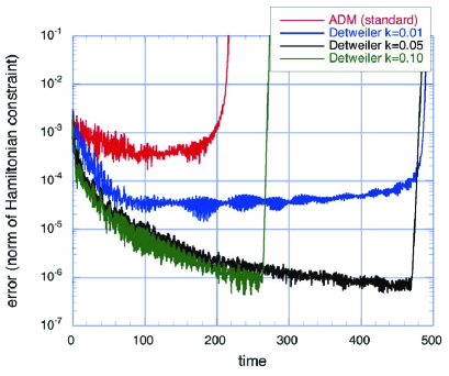
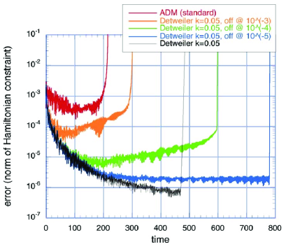
Figure 7: Demonstration of numerical evolutions between adjusted ADM systems; especially the standard ADM system and Detweiler’s modified ADM system. The L2 norm of the constraints ${\cal H}^{ADM}$ is plotted in the function of time. The model is propagation of Teukolsky wave in the periodical 3-dimensional box. $k$ is the parameter in Detweiler’s adjustment [$k_{L}$ in eq.(49)-(52)], with fixed-$k$ cases (left panel) and with fixed-and-turnoff-$k$ cases (right panel). We see the life-time of simulation becomes four-times longer than the standard ADM by tuning the parameter $k$.

We show two examples of adjustments here. Several others are shown in Table 3 of adjADMsch .

1. The standard ADM vs. original ADM
   The first comparison is to show the differences between the standard ADM ADM-York and the original ADM system ADM (see §II.1). In the notation of (44) and (45), the adjustment,

   $$R_{ij}=\kappa_{F}\alpha\gamma_{ij},$$ (48)

   (and set the other multipliers zero) will distinguish two, where $\kappa_{F}$ is a constant. Here $\kappa_{F}=0$ corresponds to the standard ADM (no adjustment), and $\kappa_{F}=-1/4$ to the original ADM (without any adjustment to the canonical formulation by ADM). As one can check by (46) and (47) adding $R_{ij}$ term keeps the constraint propagation in a first-order form. Frittelli Fri-con (see also adjADM ) pointed out that the hyperbolicity of constraint propagation equations is better in the standard ADM system. This stability feature is also confirmed numerically, and we set our CAF conjecture so as to satisfy this difference.

2. Detweiler type
   Detweiler detweiler found that with a particular combination, the evolution of the energy norm of the constraints, ${\cal H}^{2}+{\cal M}^{2}$, can be negative definite when we apply the maximal slicing condition, $K=0$. His adjustment can be written in our notation in (44) and (45), as

   $$P_{ij} = -\kappa_{L}\alpha^{3}\gamma_{ij},$$ (49)

   $$R_{ij} = \kappa_{L}\alpha^{3}(K_{ij}-(1/3)K\gamma_{ij}),$$ (50)

   $$S^{k}{}_{ij} = \kappa_{L}\alpha^{2}[{3}(\partial_{(i}\alpha)\delta_{j)}^{k}-(\partial_{l}\alpha)\gamma_{ij}\gamma^{kl}],$$ (51)

   $$s^{kl}{}_{ij} = \kappa_{L}\alpha^{3}[\delta^{k}_{(i}\delta^{l}_{j)}-(1/3)\gamma_{ij}\gamma^{kl}],$$ (52)

   everything else is zero, where $\kappa_{L}$ is a multiplier. Detweiler’s adjustment, (49)-(52), does not put constraint propagation equation to a first order form, so we cannot discuss hyperbolicity or the characteristic speed of the constraints. From perturbation analysis on Minkowskii and Schwarzschild space-time, we confirmed that Detweiler’s system provides better accuracy than the standard ADM, but only for small positive $\kappa_{L}$.

We made various predictions how additional adjusted terms will change the constraint propagation adjADM ; adjADMsch . In that process, we applied CAF analysis for Schwarzschild spacetime, and searched that when and where the negative real or non-zero imaginary eigenvalues of the homogenized constraint propagation matrix appear, and how they depend on the choice of coordinate system and adjustments. We found that there is a constraint-violating mode near the horizon for the standard ADM formulation, and that constraint-violating mode can be suppressed by adjusting equations and by choosing an appropriate gauge conditions.

III.2.2 Numerical demonstrations and remarks

Systematic numerical comparisons are in progress, and we show two sample plots here. Figure 7 is the case of Teukolsky wave Teukolskywave propagation under 3-dimensional periodic boundary condition. Both the standard ADM system and Detweiler system [one of the adjusted ADM system with adjustments (49)-(52)] are compared with the same numerical parameters. Plots are the L2 norm of the Hamiltonian constraint ${\cal H}^{ADM}$, i.e. the violation of constraints, and we see the life-time of the standard ADM evolution ends up at $t=200$. However, if we chose a particular value of $\kappa_{L}$ [multiplier in (49)-(52)], we observe that violation of constraints is reduced than the standard ADM case, and simulation can continue longer than that (left panel). If we further tuned $\kappa_{L}$, say turn-off to $\kappa_{L}=0$ when the total L2 norm of ${\cal H}^{ADM}$ is small, then we can see that the constraint violation is somewhat maintained at a small level and more long-term stable simulation is available (right panel).

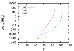
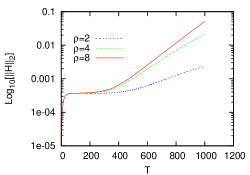
Figure 8: The one-dimensional gauge-wave test with the BSSN system (left) and the adjusted BSSN system (right) in the $\tilde{A}$-equation (53). The L2 norm of ${\cal H}$, rescaled by the resolution parameter $\rho^{2}/4$, are plotted with a function of the crossing-time. The wave amplitude is set to 0.01, and we chose the adjustment parameter $\kappa_{A}=0.005$. The BSSN system loses convergence at the early time, near the 20 crossing-time and it will produce the blow-ups of the calculation in the end, while in the adjusted version we see the higher resolution runs show convergence longer, i.e., the 300 crossing-time in ${\cal H}$ and all runs can stably evolve up to the 1000 crossing-time.

During the comparisons of adjustments, we found that it is necessary to create time asymmetric structure of evolution equations in order to force the evolution on to the constraint surface. There are infinite ways of adjusting equations, but we found that if we follow the next guideline, then such an adjustment will give us time asymmetric evolution.

$\Box$Trick to obtain asymptotically constrained system:
$=$ Break the time reversal symmetry (TRS) of the evolution equation.

1. Evaluate the parity of the evolution equation.
   By reversing the time ($\partial_{t}\rightarrow-\partial_{t}$), there are variables which change their signatures (parity $(-)$) [e.g. $K_{ij},\partial_{t}\gamma_{ij},{\cal M}_{i},\cdots$], while not (parity $(+)$) [e.g. $g_{ij},\partial_{t}K_{ij},{\cal H},\cdots$].

2. Add adjustments which have different parity of that equation.
   For example, for the parity $(-)$ equation $\partial_{t}\gamma_{ij}$, add a parity $(+)$ adjustment $\kappa{\cal H}$. $\qquad\Box$

One of our criteria, the negative real CAFs, requires breaking the time-symmetric features of the original evolution equations. Such CAFs are obtained by adjusting the terms which break the TRS of the evolution equations, and this is available even at the standard ADM system.

III.3 Applications 2: Adjusted BSSN formulations

III.3.1 Constraint propagation analysis of the BSSN equations

In order to understand the stability property of the BSSN system, we studied the structure of the evolution equations, (17)-(21), in detail, especially how the modifications using the constraints, (22)-(26), affect to the stability adjBSSN . We investigated the signature of the eigenvalues of the constraint propagation equations, and explained that the standard BSSN dynamical equations are balanced from the viewpoint of constrained propagations, including a clarification of the effect of the replacement using the momentum constraint equation, which was reported by Alcubierre et al. potsdam9908 .

Moreover, we predicted that several combinations of modifications have a constraint-damping nature, and named them adjusted BSSN systems. Several adjusted BSSN systems are proposed in Table II of adjBSSN .

Yo et al. YBS immediately applied one of our proposals to their simulations of stationary rotating black hole, and reported that one adjustment was contributed to maintain their evolution of Kerr black hole ($J/M$ up to $0.9M$) for long time ($t\sim 6000M$). Their results also indicates that the evolved solution is closed to the exact one, that is, the constrained surface.

Now, let us make clear some current technical tips listed in §II.2.2 using constraint propagation analysis.

• Trace-out $A_{ij}$ technique can be explained that the violation of ${\cal A}$-constraint (25) affects to all other constraint violations. (See the full set of constraint propagation equations in Appendix of adjBSSN .)

• Replacement of $\tilde{\Gamma}^{i}$ enables to maintain ${\cal G}$-constraint (24) that delays the violation of ${\cal H}^{BSSN}$ and ${\cal M}^{BSSN}_{i}$. (Again, the statement comes from the full set of constraint propagation equations. )

III.3.2 Numerical Demonstrations

We recently presented our numerical comparisons of 3 kinds of adjusted BSSN formulationadjBSSNnum . We performed three testbeds: gauge-wave, linear wave, and Gowdy-wave tests, proposed by the Mexico workshop mexico1 on the formulation problem of the Einstein equations. We observed that the signature of the proposed Lagrange multipliers are always right and the adjustments improve the convergence and stability of the simulations. When the original BSSN system already shows satisfactory good evolutions (e.g., linear wave test), the adjusted versions also coincide with those evolutions; while in some cases (e.g., gauge-wave or Gowdy-wave tests) the simulations using the adjusted systems last 10 times as long as those using the original BSSN equations.

Figure 8 show the comparison between the (plain) BSSN system and the adjusted BSSN system in $\tilde{A}$-equation using the momentum constraint:

$$\partial_{t}\tilde{A}_{ij}=\partial^{B}_{t}\tilde{A}_{ij}+\kappa_{A}\alpha\tilde{D}_{(i}{\cal M}_{j)},$$ (53)

where $\kappa_{\cal A}$ is predicted (from the eigenvalue analysis) to be positive in order to damp the constraint violations. The testbed is one-dimensional gauge-wave; the trivial Minkowski space-time but sliced with the time-dependent 3-metric. The poor performance of the plain BSSN system of this test has been already reported Jansen:2003uh , and one remedy is to apply the 4th-order finite differencing scheme Zlochower:2005bj . The plots show that our adjusted system also improve the life-time of the plain BSSN simulation at least 10 times longer with better convergence.

IV Outlook

IV.1 What we have achieved

We reviewed recent efforts to the formulation problem of numerical relativity; the problem to find out a robust system against constraint violations. We categorized the approaches into

• The standard ADM formulation (§II.1),

• The BSSN formulation (§II.2),

• Hyperbolic formulations (§II.3), and

• Asymptotically constrained formulations (§II.4).

Most of the numerical relativity groups now use the BSSN set of equations which are obtained empirically. A dramatic announcement of the success of binary black-hole simulations rushes the community to follow that recipe. Actually we are not yet completely understanding why the current set of BSSN equations together with particular combinations of gauge condition works well. Several explanations are applied based on the hyperbolic formulation scheme, but as we viewed there are not yet satisfactory.

Our approach, on the other hand, tries to construct an evolution system that has its constraint surface as an attractor. Our unified view is to understand the evolution system by evaluating its constraint propagation. Especially we proposed to analyze the constraint amplification factors which are the eigenvalues of the homogenized constraint propagation equations. We analyzed the system based on our conjecture whether the constraint amplification factors suggest the constraint to decay/propagate or not. We concluded that

• The constraint propagation features become different by simply adding constraint terms to the original evolution equations (we call this the adjustment of the evolution equations).

• There is a constraint-violating mode in the standard ADM evolution system when we apply it to a single non-rotating black hole space-time, and its growth rate is larger near the black-hole horizon.

• Such a constraint-violating mode can be killed if we adjust the evolution equations with a particular modification using constraint terms. An effective guideline is to adjust terms as they break the time-reversal symmetry of the equations.

• Our expectations are borne out in simple numerical experiments using the Maxwell, Ashtekar, and ADM systems. However the modifications are not yet perfect to prevent non-linear growth of the constraint violation.

• We understand why the BSSN formulation works better than the ADM one in the limited case (perturbation analysis in the flat background), and further we proposed modified evolution equations along the lines of our previous procedure. Some of these proposed adjusted systems are numerically confirmed to work better than the standard BSSN system.

The common key to the problem is how to adjust the evolution equations with constraints. Any adjusted systems are mathematically equivalent if the constraints are completely satisfied, but this is not the case for numerical simulations. Replacing terms with constraints is one of the normal steps when people re-formulate equations in a hyperbolic form.

In summary, let me answer the following three questions:

• What is the guiding principle for selecting evolution equations for simulations in GR?
  –The key is to analyze the constraint propagation equation of the system.

• Why many groups use the BSSN equations?
  –Because people just rush, not to be late to others.

• Are there an alternative formulation better than the BSSN?
  –Yes, there are. But we do not know which is the best one yet.

IV.2 Future directions

If we say the final goal of this project is to find a robust evolution system against violation of constraints, then the recipe should be a combination of (a) formulations of the evolution equations, (b) choice of gauge conditions, (c) treatment of boundary conditions, and (d) numerical integration methods. We are now in the stages of solving these mixed puzzles.

Recent attentions to higher dimensional space-time studies are waiting for numerical researches, but it is known that the formulation problem also exists in higher dimensional cases ndimCP .

We have written this review from the viewpoint that the general relativity is a constrained dynamical system. This is not a proper problem in general relativity, but there is also in many physical systems such as electrodynamics, magnetohydrodynamics, molecular dynamics, mechanical dynamics. Therefore, sharing and interacting the thoughts between different fields will definitely accelerate the progress.

The ideal almighty algorithm to solve all the problems may not exist, but the author believe that our final numerical recipe is somewhat an automatic system, and hope that numerical relativity turns to be an easy toolkit for everyone in near future.

References

- (1) A. Abrahams, A. Anderson, Y. Choquet-Bruhat, and J. W. York, Jr., Phys. Rev. Lett. 75, 3377 (1995); Class. Quant. Grav. 14, A9 (1997).
- (2) M. Alcubierre, Phys. Rev. D 55, 5981 (1997).
- (3) M. Alcubierre, Proceedings of the 17th International Conference on General Relativity and Gravitation (GR17), gr-qc/0412019.
- (4) M. Alcubierre, G. Allen, B. Bruegmann, E. Seidel and W-M. Suen, Phys. Rev. D 62, 124011 (2000).
- (5) M. Alcubierre, B. Bruegmann, T. Dramlitsch, J.A. Font, P. Papadopoulos, E. Seidel, N. Stergioulas, and R. Takahashi, Phys. Rev. D 62, 044034 (2000).
- (6) M. Alcubierre and J. Massó, Phys. Rev. D 57, R4511 (1998).
- (7) M. Alcubierre et al. (Mexico Numerical Relativity Workshop 2002 Participants) Class. Quant. Grav. 21, 589 (2004).
- (8) A. Alekseenko and D. Arnold, Phys. Rev. D 68, 064014 (2003).
- (9) A. Anderson, Y. Choquet-Bruhat, J. W. York, Jr., Topol. Methods in Nonlinear Analysis, 10, 353 (1997).
- (10) A. Anderson and J. W. York, Jr, Phys. Rev. Lett. 82, 4384 (1999).
- (11) P. Anninos, D. Bernstein, S. Brandt, J. Libson, J. Massó, E. Seidel, L. Smarr, W-M. Suen, and P. Walker, Phys. Rev. Lett. 74, 630 (1995).
- (12) R. Arnowitt, S. Deser and C.W. Misner, in Gravitation: An Introduction to Current Research, ed. by L.Witten, (Wiley, New York, 1962).
- (13) A. Ashtekar, Phys. Rev. Lett. 57, 2244 (1986); Phys. Rev. D36, 1587 (1987).
- (14) J. G. Baker, et al. Phys. Rev. Lett. 96, 111102 (2006); Phys. Rev. D 73, 104002 (2006).
- (15) T. W. Baumgarte and S. L. Shapiro, Phys. Rev. D 59, 024007 (1999).
- (16) T. W. Baumgarte and S.L. Shapiro, Phys. Rept. 376, 41 (2003).
- (17) J. M. Bardeen, L. T. Buchman, Phys. Rev. D 65, 064037 (2002).
- (18) C. Bona, T. Ledvinka, C. Palenzuela, Phys. Rev. D 66, 084013 (2002); C. Bona, T. Ledvinka, C. Palenzuela, and Žáček, ibid. 67, 104005 (2003); ibid. 69, 064036 (2004).
- (19) C. Bona, J. Massó, Phys. Rev. D 40, 1022 (1989); Phys. Rev. Lett. 68, 1097 (1992).
- (20) C. Bona, J. Massó, E. Seidel and J. Stela, Phys. Rev. Lett. 75, 600 (1995); Phys. Rev. D 56, 3405 (1997).
- (21) C. Bona, J. Massó, E. Seidel, and P. Walker, gr-qc/9804052.
- (22) O. Brodbeck, S. Frittelli, P. Hübner, and O.A. Reula, J. Math. Phys. 40, 909 (1999).
- (23) B. Bruegmann, Proceedings of GRG18 (at Sydney, Australia, 2007), to be published.
- (24) L. Buchman and O. Sarbach, Class. Quant. Grav. 23, 6709 (2006).
- (25) G. Calabrese, J. Pullin, O. Sarbach, and M. Tiglio, Phys. Rev. D 66 064011 (2002); ibid. 66, 041501 (2002).
- (26) M. Campanelli, C. O. Lousto, P. Marronetti, Y. Zlochower, Phys. Rev. Lett. 96, 111101 (2006); M. Campanelli, C. O. Lousto, Y. Zlochower, Phys. Rev. D 73, 061501(R) (2006).
- (27) M. W. Choptuik, Phys. Rev. D 44, 3124 (1991).
- (28) M. W. Choptuik, Phys. Rev. Lett. 70, 9 (1993).
- (29) Y. Choquet-Bruhat and J. W. York, Jr., C. R. Acad. Sc. Paris 321, Série I, 1089, (1995).
- (30) S. Detweiler, Phys. Rev. D 35, 1095 (1987).
- (31) P. Diener, et al. Phys. Rev. Lett. 96 (2006) 121101.
- (32) J. Frauendiener and T. Vogel, Class. Quant. Grav. 22 1769 (2005).
- (33) H. Friedrich, Proc. Roy. Soc. A 375, 169 (1981); ibid. 378, 401 (1981).
- (34) H. Friedrich, Commun. Math. Phys. 91, 445 (1983).
- (35) H. Friedrich and G. Nagy, Comm. Math. Phys. 201, 619 (1999).
- (36) S. Frittelli, Phys. Rev. D 55, 5992 (1997).
- (37) S. Frittelli and R. Gomez, J. Math. Phys. 41, 5535 (2000).
- (38) S. Frittelli and O. A. Reula, Phys. Rev. Lett. 76, 4667 (1996).
- (39) D. Garfinkle, C. Gundlach, D. Hilditch, arXiv:0707.0726
- (40) C. Gundlach, G. Calabrese, I. Hinder, and J. M. Martin-Garcia, Class. Quant. Grav. 22, 3767 (2005).
- (41) C. Gundlach and J. M. Martin-Garcia, Phys. Rev. D 70, 044031 (2004); ibid.74, 024016 (2006).
- (42) S. D. Hern, PhD thesis, gr-qc/0004036.
- (43) H. Heyer and O. Sarbach, Phys. Rev. D 70, 104004 (2004).
- (44) N. Jansen, B. Bruegmann and W. Tichy, Phys. Rev. D 74, 084022 (2006).
- (45) L. E. Kidder, M. A. Scheel, S. A. Teukolsky, Phys. Rev. D 64, 064017 (2001).
- (46) K. Kiuchi and H. Shinkai, Phys. Rev. D 77, 044010 (2008).
- (47) H-O. Kreiss, O. Reula, O. Sarbach and J. Winicour, Class. Quant. Grav. 24, 5973 (2007).
- (48) L. Lindblom and M. Scheel, Phys. Rev. D 66, 084014 (2002).
- (49) M. Miller, gr-qc/0008017.
- (50) C. W. Misner, K. S. Thorne, J. A. Wheeler, Gravitation, (Freeman, N.Y., 1973).
- (51) G. Nagy, O.E. Ortiz and O.A. Reula, Phys. Rev. D 70, 044012 (2004).
- (52) T. Nakamura and K. Oohara, in Frontiers in Numerical Relativity edited by C. R. Evans, L. S. Finn, and D. W. Hobill (Cambridge Univ. Press, Cambridge, England, 1989).
- (53) T. Nakamura, K. Oohara and Y. Kojima, Prog. Theor. Phys. Suppl. 90, 1 (1987).
- (54) F. Pretorius, Phys. Rev. Lett. 95 (2005) 121101; Class. Quant. Grav. 23 (2006) S529.
- (55) F. Pretorius, arXiv:0710.1338
- (56) M. Ruiz, O. Rinne and O. Sarbach, Class. Quant. Grav. 24, 6349 (2007).
- (57) O. Sarbach, G. Calabrese, J. Pullin, and M. Tiglio, Phys. Rev. D 66, 064002 (2002).
- (58) M. A. Scheel, T. W. Baumgarte, G. B. Cook, S. L. Shapiro, S. A. Teukolsky, Phys. Rev. D 56, 6320 (1997);
- (59) M. A. Scheel, T. W. Baumgarte, G. B. Cook, S. L. Shapiro, S. A. Teukolsky, Phys. Rev. D 58, 044020 (1998).
- (60) S. L. Shapiro and S. A. Teukolsky, Phys. Rev. Lett. 66, 994 (1991).
- (61) M. Shibata and T. Nakamura, Phys. Rev. D 52, 5428 (1995).
- (62) H. Shinkai and G. Yoneda, Phys. Rev. D 60, 101502 (1999).
- (63) H. Shinkai and G. Yoneda, Class. Quant. Grav. 17, 4799 (2000).
- (64) H. Shinkai and G. Yoneda, Class. Quant. Grav. 19, 1027 (2002).
- (65) H. Shinkai and G. Yoneda, in Progress in Astronomy and Astrophysics (Nova Science Publ). The manuscript is available as gr-qc/0209111.
- (66) H. Shinkai and G. Yoneda, Gen. Rel. Grav. 36, 1931 (2004).
- (67) F. Siebel and P. Hübner, Phys. Rev. D 64, 024021 (2001).
- (68) L. Smarr, J. W. York, Jr., Phys. Rev. D 17, 2529 (1978).
- (69) C. F. Sopuerta, U. Sperhake, P. Laguna, Class. Quant. Grav. 23 (2006) S579.
- (70) H. Stephani, D. Kramer, M. MacCallum, C. Hoenselaers, and E. Herlt, Exact Solutions to Einstein’s Field Equations Second ed., (Cambridge, Cambridge Univ. Press, 2003).
- (71) J. M. Stewart, Class. Quant. Grav. 15, 2865 (1998).
- (72) S. A. Teukolsky, Phys. Rev. D 26, 745 (1982).
- (73) H-J. Yo, T. W. Baumgarte and S. L. Shapiro, Phys. Rev. D 66, 084026 (2002).
- (74) G. Yoneda and H. Shinkai, Phys. Rev. Lett. 82, 263 (1999); Int. J. Mod. Phys. D. 9, 13 (2000).
- (75) G. Yoneda and H. Shinkai, Class. Quant. Grav. 18, 441 (2001).
- (76) G. Yoneda and H. Shinkai, Phys. Rev. D 63, 124019 (2001).
- (77) G. Yoneda and H. Shinkai, Phys. Rev. D 66, 124003 (2002).
- (78) G. Yoneda and H. Shinkai, Class. Quant. Grav. 20, L31 (2003).
- (79) J. W. York, Jr., in Sources of Gravitational Radiation, ed. by L. Smarr, (Cambridge, 1979).
- (80) Y. Zlochower, J. G. Baker, M. Campanelli and C. O. Lousto, Phys. Rev. D 72, 024021 (2005)