Straight Skeletons of Three-Dimensional Polyhedra

Abstract

This paper studies the straight skeleton of polyhedra in three dimensions. We first address voxel-based polyhedra (polycubes), formed as the union of a collection of cubical (axis-aligned) voxels. We analyze the ways in which the skeleton may intersect each voxel of the polyhedron, and show that the skeleton may be constructed by a simple voxel-sweeping algorithm taking constant time per voxel. In addition, we describe a more complex algorithm for straight skeletons of voxel-based polyhedra, which takes time proportional to the area of the surfaces of the straight skeleton rather than the volume of the polyhedron. We also consider more general polyhedra with axis-parallel edges and faces, and show that any $n$-vertex polyhedron of this type has a straight skeleton with $O(n^{2})$ features. We provide algorithms for constructing the straight skeleton, with running time $O(\min(n^{2}\log n,k\log^{O(1)}n))$ where $k$ is the output complexity. Next, we discuss the straight skeleton of a general nonconvex polyhedron. We show that it has an ambiguity issue, and suggest a consistent method to resolve it. We prove that the straight skeleton of a general polyhedron has a superquadratic complexity in the worst case. Finally, we report on an implementation of a simple algorithm for the general case.

1 Introduction

The straight skeleton is a geometric construction that reduces two-dimensional shapes—polygons—to one-dimensional sets of line segments approximating the same shape. It is defined in terms of an offset process in which edges move inward, remaining straight and meeting at vertices. When a vertex meets an offset edge, the process continues within the two pieces so formed. The straight line segments traced out by vertices during this offset process define the straight skeleton. Introduced in 1995 by Aichholzer et al. [2, 1], the two-dimensional straight skeleton has since found many applications, including surface folding [11], offset curve construction [15], interpolation of three-dimensional surfaces from cross-section contours [4], automated interpretation of geographic data [17], polygon decomposition [24], and graph drawing [3]. Compared to other well-known types of skeleton, the straight skeleton is more complex to compute [15, 7], but its simple geometric form, comprised exclusively of line segments, offers advantages in applications. The best known alternative, the medial axis [6], consists of both linear and quadratic curve segments. Thus, of the two, only the straight skeleton characterizes the shape of a polygon while preserving its linear nature.

It is natural, then, to try to extend algorithms for straight skeleton construction to three dimensions. In three dimensions, a skeleton is a two-dimensional approximation of a three-dimensional shape such as a polyhedron. The most well-known type of three-dimensional skeleton, the medial axis, has found applications, for instance, in mesh generation [20] and surface reconstruction [5]. Unlike its two-dimensional counterpart, the 3D medial axis can be quite complex, both combinatorially and geometrically. Thus, we would like an alternative way to characterize the shape of three-dimensional polyhedra using a simpler type of two-dimensional skeleton.

1.1 Related Prior Work

Despite the large amount of work on 2D straight skeletons cited above, we are not aware of any prior work on 3D straight skeletons, other than Demaine et al. [10], who mention the existence and basic properties of 3D straight skeletons, but do not study them in any detail with respect to their algorithmic, combinatorial, or geometric properties.

Held [18] showed that in the worst case, the complexity of the medial axis of a convex polyhedron of complexity $n$ is $\Omega(n^{2})$, which implies a similar bound for the 3D straight skeleton. Perhaps the most relevant prior work is on shape characterization using the 3D medial axis. This structure is defined from a 3D polyhedron by considering each face, edge, and vertex as being a distinct object and then constructing the 3D Voronoi diagram of this set of objects. Thus, the medial axis is the loci of points in $\Bbb R^{3}$ that are equidistant to at least two objects. The best known upper bound for its combinatorial complexity is $O(n^{3+\epsilon})$ [21], for any fixed constant $\epsilon>0$, and even for the special case of lines in space it is a well-known open problem in computational geometry whether the Voronoi diagram (a space subdivision having the medial axis as its boundary) has subcubic combinatorial complexity [8, 19]. Additionally, the medial axis consists of intersecting pieces of planes and conic surfaces, presenting significant complications to algorithms that attempt to construct 3D medial axes.

Because of these drawbacks, a number of researchers have studied algorithms for computing approximate 3D medial axes. Sherbrooke et al. [23] take a numerical approach, giving an algorithm that traces out the curved edges of the 3D medial skeleton. Culver et al. [9] also design a curve-tracing algorithm, but they use exact arithmetic to compute an exact representation of a 3D medial axis. In both cases, the running time depends on both the combinatorial and geometric complexity of the medial axis. Foskey et al. [16] study an approximation based on relaxed distance calculations. In particular, they construct an approximate medial axis using a voxel-based approach that runs in time $O(nV)$, where $n$ is the number of features of the input polyhedron and $V$ is the volume of the voxel mesh that contains it. Sheehy et al. [22] instead take the approach of using the 3D Delaunay triangulation of a cloud of points on the surface of the input polyhedron to compute and approximate 3D medial axis. Likewise, Dey and Zhao [12] study the 3D medial axis as a subcomplex of the Voronoi diagram of a sampling of points approximating the input polyhedron.

1.2 Our Results

In this paper we provide the following results.

• We study the straight skeleton of orthogonal polyhedra formed as unions of cubical voxels. We analyze the ways in which the skeleton may intersect each voxel of the polyhedron, and show that the skeleton may be constructed by a simple voxel sweeping algorithm taking constant time per voxel.

• We describe a more complex algorithm for straight skeletons of voxel-based polyhedra, which, rather than taking time proportional to the volume of the polyhedron takes time proportional to the area of the straight skeleton or, equivalently, the number of voxels it intersects.

• We consider more general polyhedra with axis-parallel edges and faces, and show that any $n$-vertex polyhedron of this type has a straight skeleton with $O(n^{2})$ features. We provide two algorithms for constructing the straight skeleton, resulting in a combined running time of $O(\min(n^{2}\log n,k\log^{O(1)}n))$, where $k$ is the output complexity.

• We discuss the difficulties of unambiguously defining straight skeletons for non-axis-aligned polyhedra and suggest a consistent method for resolving these ambiguities. We show that a general polyhedron, the straight skeleton can, in the worst case, have superquadratic complexity. Thus, straight skeletons are strictly simpler for orthogonal polyhedra than they are for more general polyhedra. We also describe a simple algorithm for computing the straight skeleton in the general case.

2 Voxel Polyhedra

In this section we consider the case in which the polyhedron is a polycube, that is, a rectilinear polyhedron all of whose vertices have integer coordinates. The “cubes” making up the polyhedron are also called voxels.

For voxels, and more generally for orthogonal polyhedra, the straight skeleton is a superset of the $L_{\infty}$ Voronoi diagram; the added boundaries in the straight skeleton resolve any ambiguities concerning which cells of the diagram belong to which features of the input polyhedron. Due to this relationship with Voronoi diagrams, the straight skeleton is significantly easier to compute for orthogonal inputs than in the general case.

As in the general case, the straight skeleton of a polycube can be modeled by offsetting the boundary of the polycube inward, and tracing the movement of the boundary. During this sweep, the boundary forms a moving front (or fronts) whose features are faces, edges, and vertices. An edge can be either convex or concave, while a vertex can be convex, concave, or a saddle. In the course of this process, features may disappear or appear.

The sweep starts at time 0; at this time the front is the boundary of the polycube. In the first time unit we process all the voxels adjacent to the boundary. In the $i$th round (for $i\geq 1$) we process all the voxels adjacent to voxels processed in the $(i-1)$st round, that have never been processed before. Processing a voxel means the computation of the piece of the skeleton lying within (or on the boundary) of the voxel. During this process, the polycube is shrunk, and may be broken into several components if it is not convex. The process continues for every piece separately until it vanishes, that is, there are no more voxels to process.

2.1 A Volume Proportional-Time Algorithm

Theorem 2.1

The combinatorial complexity of the straight skeleton of a polycube of volume $V$ is $O(V)$. The skeleton can be computed in $O(V)$ time.

Proof

We prove the two parts of the theorem simultaneously by analyzing the skeleton computation procedure, in which the boundary of the polycube is swept inward and the movement of its features is traced. We analyze separately the time needed to find the voxels processed in each sweep step and the time needed to process each voxel. We show that the entire sweep can be performed in time linear in the number of voxels, the complexity of the skeleton within every voxel is constant, and the portion of the skeleton within every voxel can be computed in constant time.

The sweep starts at time 0 at the boundary of the polycube. In the first round we process all the voxels adjacent to the boundary. In the $i$th round (for $i\geq 1$) we process all the voxels adjacent to voxels processed in the $(i-1)$st round, that have never been processed before. When sweeping the boundary inward during one round of the process, each feature of the boundary (vertex, edge, or face) moves inward one L_∞ unit. For clarity of exposition, we will analyze the process within eighths of voxels instead of full voxels. This will reduce the number of possible cases, since we will have to consider all combinations of vertices/edges/facets hit by the moving front(s) only on three facets instead of the six facets that a full voxel can be hit simultaneously on. Consider an eighth of the voxel that is about to be swept by the moving front(s). This “subvoxel” can be hit in many combinations of its corner vertex, the three edges adjacent to this corner, and the three faces adjacent to this corner. Moreover, it may be hit by multiple portions of the moving front in a single feature of the subvoxel, in two features, one containing the other, or multiple features with more complex containment relations. Nevertheless, the number of different cases is finite, and a preprocessed look-up table can be used to determine in constant time the structure of the piece of the straight skeleton within each subvoxel. The complexity of the skeletal piece (within a voxel) is also constant. Figures 1(a–h)

\begin{picture}(3324.0,3387.0)(3589.0,-5236.0)\end{picture}	\begin{picture}(3409.0,3409.0)(3589.0,-5258.0)\end{picture}	\begin{picture}(3494.0,3409.0)(3504.0,-5258.0)\end{picture}	\begin{picture}(3494.0,3420.0)(3504.0,-5258.0)\end{picture}	\begin{picture}(3494.0,3409.0)(3504.0,-5258.0)\end{picture}	\begin{picture}(3494.0,3409.0)(3504.0,-5258.0)\end{picture}
(a) Vertex	(b) Edge	(c) Two edges	(d) Three edges	(e) Face	(f) Face and edge

\begin{picture}(3494.0,3494.0)(3504.0,-5258.0)\end{picture}	\begin{picture}(3494.0,3494.0)(3504.0,-5258.0)\end{picture}		\begin{picture}(3388.0,3388.0)(3557.0,-5205.0)\end{picture}	\begin{picture}(3324.0,3324.0)(3589.0,-5173.0)\end{picture}
(g) Two faces	(h) Three faces	(i) Overlapping edges	(j) Overlapping faces	(k) Overlapping edge and face

Figure 1: Cases of straight skeleton within a subvoxel (a-h) or voxel (i-k).

show the creation of a skeletal piece in the interior of a subvoxel in simple cases. The features through which the moving fronts enter the subvoxel are shown enlarged. Figures 1(i–k) show (in full voxels) a few cases of overlapping entry features.

To recap, the algorithm processes all voxels in layers, in a total of $\Theta(V)$ voxel operations, each of which takes constant time and contributes a constant amount of skeletal features. The algorithm terminates when there are no more voxels to process and the entire straight skeleton of the polycube has been computed.

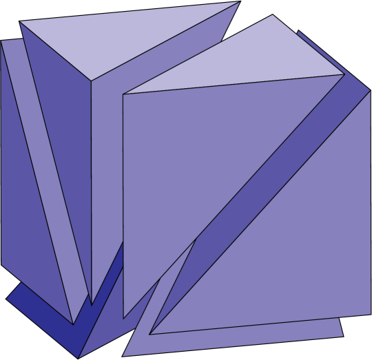
Figure 2: Partitioning a subvoxel into tetrahedra.

\begin{picture}(6549.0,2424.0)(589.0,-3973.0)\end{picture}	\begin{picture}(3666.0,3966.0)(3568.0,-5194.0)\end{picture}
(a)	(b)

Figure 3: A polycube of volume $V$ whose skeleton has complexity $\Theta(V)$.

A unified way to look at all cases above is to partition a voxel, as above, to eight subvoxels, and then partition each subvoxel into six tetrahedra each of which is the convex hull of one of the six three-edge paths connecting the subvoxel’s integer vertex with its half-integer vertex (Figure 3). Thus, every voxel is partitioned into 48 tetrahedra. All skeletal cells are unions of these tetrahedra, and the surface of the skeleton is composed of their boundary triangles. By maintaining “visited” marks on the tetrahedra and on the integer and half-integer vertices, one can sweep the wavefront and compute the revealed pieces of the skeleton.

Many simple examples show that the sweeping algorithm is worst-case optimal up to constant factors, since in the worst case the complexity of a polycube made of $V$ voxels is $\Theta(V)$. One such example, shown in Figure 3(a), is made of a flat layer of cubes (not shown), with a grid of supporting “legs,” each a single cube. Thus, the number of legs is about one fifth of the total number of voxels. The skeleton of this object has features within every leg, as shown in Figure 3(b) (the bottom of a leg corresponds to the right side of the figure).

2.2 Output-Sensitive Voxel Sweep

The straight skeleton of a polycube, as constructed by the previous algorithm, contains features within some voxels, but other voxels may not participate in the skeleton; nevertheless, the algorithm must consider all voxels and pay in its running time for them. In this section we outline a more efficient algorithm that computes the straight skeleton in time proportional only to the number of voxels containing skeleton features, or equivalently, in time proportional to the surface area of the straight skeleton rather than its volume. Necessarily, we assume that the input polycube is provided as a space-efficient boundary representation rather than as a set of voxels, for otherwise simply scanning the input would take more time than we wish to spend.

Our algorithm consists of an outer loop, in which we advance the moving front of the polycube boundary one time step at a time, and an inner loop, in which we capture all features of the straight skeleton formed in that time step. During the algorithm, we maintain at each step a representation of the moving front, as a collection of polygons having orthogonal and diagonal edges. As long as each operation performed in the inner and outer loops of the algorithm can be charged against straight skeleton output features, the total time will be proportional to the output size.

In order to avoid the randomization needed for hashing, several steps of our algorithm will use as a data structure a direct-addressed lookup table, which we summarize in the following lemma:

Lemma 1

In time proportional to the boundary of an input polycube, we may initialize a data structure that can repeatedly take as input a collection of objects, indexed by integers within the range of coordinate values of the polycube vertices, and produce as output a graph, the vertices of which are sets of objects that have equal indices and the edges of which are pairs of sets with index values that differ by one. The time per operation is proportional to the number of objects given as input.

Proof

We use an array, indexed by the given integer values, containing a list of objects in each array cell. Initially, we set all lists to empty. To handle a given collection of objects, we place each object in the list given by the object’s index, and create a list $L$ of nonempty index values as we do so; each time we add an object to an empty list, we add that list’s index to $L$. We then create a graph having as its vertices the lists indexed by $L$; for each vertex we search the array for the two adjacent indices and create the appropriate graph edges. Finally, we use $L$ to replace each nonempty list of the array with a new empty list.

In more detail, in each step of the outer loop of the algorithm, we perform the following steps:

1. Advance each face of the wavefront one unit inward. In this advancement process, we may detect events in which a wavefront edge shrinks to a point, forming a straight skeleton vertex. However, events involving pairs of features that are near in space but far apart on the wavefront may remain undetected. Thus, after this step, the wavefront may include overlapping pairs of coplanar oppositely-moving faces.

2. For each plane containing faces of the new wavefront boundary, detect pairs of faces that overlap within that plane, and find the features in which two overlapping face edges intersect or in which a vertex of one face lies in the interior of another face. This step can be performed as a sequence of smaller steps:

   • Group coplanar faces of the wavefront using the data structure of Lemma 1.

   • Within each plane $P$, form a set $S_{P}$ of the wavefront edges intersected with each voxel. We assume that the plane is parallel to the $xy$ plane; the $xz$ and $yz$ cases are handled symmetrically.

   • For each plane $P$, use Lemma 1 to form a graph $G_{P}$; vertices in $G_{P}$ represent sets of edges in $S_{P}$ with the same left $x$-coordinate, and edges in $G_{P}$ connect sets with consecutive $x$-coordinates. The connected components of this graph are paths representing subsets of wavefront features that might possibly interact with each other, sorted by their $x$-coordinates.

   • Within each connected component of each graph $G_{P}$, use the sorted order to perform a plane sweep algorithm that finds segment intersections and locates the face containing each vertex. Report as straight skeleton events each intersection between edges of different boundary faces and each vertex that belongs to a boundary face other than the one on which it is a boundary vertex.

3. In the inner loop of the algorithm, propagate straight skeleton features within each face of the wavefront from the points detected in the previous step to the rest of the face. If two faces overlap in a single plane, the previous step will have found some of the points at which they form straight skeleton vertices, but the entire overlap region will form a face of the straight skeleton. We propagate outward from the detected intersection points using depth-first-search, voxel by voxel, to determine the straight skeleton features contained within the overlap region.

In summary, we have:

Theorem 2.2

One can compute the straight skeleton of a polycube in time proportional to its surface area.

3 Orthogonal Polyhedra

We consider here a more general class of inputs than voxels: orthogonal polyhedra in which all faces are parallel to two of the coordinate axes.

3.1 Definition

As in the two-dimensional case, we define the straight skeleton of an orthogonal polyhedron $P$ by a continuous shrinking process in which a sequence of nested “offset surfaces” are formed, starting from the boundary of the given polyhedron, with each face moving inward at a constant speed. At time $t$ in this shrinking process, the offset surface $P_{t}$ for $P$ consists of the set of points at $L_{\infty}$ distance exactly $t$ from the boundary of $P$. For almost all values of $t$, $P_{t}$ will itself be a polyhedron, but at some time steps $P_{t}$ may have a non-manifold topology, possibly including flat sheets of surface that do not bound any interior region. When this happens, the evolution of the surface undergoes sudden discontinuous changes, as these surfaces vanish at time steps after $t$ in a discontinuous way. To make this notion of discontinuity more precise, we define a degenerate point of $P_{t}$ to be a point $p$ that is on the boundary of $P_{t}$, such that, for some $\delta$, and all $\epsilon>0$, $P_{t+\epsilon}$ does not contain any point within distance $\delta$ of $p$. Equivalently, a degenerate point is a point of $P_{t}$ that does not belong to the closure of the interior of $P_{t}$.

At each step in the shrinking process, we imagine the surface of $P_{t}$ as decorated with seams left over when sheets of degenerate points occur. To be more specific, suppose that $P$ contains two disjoint faces, both parallel to the $xy$ plane at the same $z$-height; then, as we shrink $P$, the corresponding faces of $P_{t}$ may grow toward each other, eventually meeting. When they do meet, they leave a seam between them. Seams can also occur when two parts of the same nonconvex face grow toward and meet each other. After a seam forms, it remains on the face of $P_{t}$ on which it formed, orthogonal to the position at which it originally formed.

We may also describe these seams in a more intrinsic, static way. Let $\Pi$ be any axis-aligned plane containing a face or faces of $P$, and let $S_{\Pi}$ be the two-dimensional straight skeleton in $\Pi$ of the exterior of these faces, not including the straight skeleton edges that touch the vertices of $P$. Then the decoration on any face $f$ of $P_{t}$, corresponding to a face of $P$ belonging to plane $\Pi$, is formed by translating $S_{\Pi}$ orthogonally into the plane of $f$ and intersecting it with $f$.

We define the straight skeleton of $P$ to be the union of three sets:

1. The points that, for some time step $t$, belong to an edge or vertex of $P_{t}$.

2. The degenerate points for $P_{t}$ for some time step $t$.

3. The points that, for some time step $t$, belong to a seam of $P_{t}$.

The straight skeleton may be viewed as a cell complex in $\Bbb R^{3}$, consisting of faces (maximal subsets of points that have a 2D neighborhood in the straight skeleton), edges (maximal line segments of points that either do not lie in a face, lie on the boundary of a face, or lie in the intersection of two or more faces), and vertices (endpoints of edges).

3.2 Complexity Bounds

As each face has at least one boundary edge, and each edge has at least one vertex, we may bound the complexity of the straight skeleton by bounding the number of its vertices. Each vertex corresponds to an event, that is, a point $p$ in space (the location of the vertex), the time $t$ for which $p$ belongs to the boundary of $P_{t}$, and the set of features of $P_{t-\epsilon}$ near $p$ for small values of $\epsilon$ that contribute to the event. We may classify events into six types.

Concave-vertex events

describe the situation in which one of the features of $P_{t-\epsilon}$ involved in the event is a concave vertex: that is, a vertex of $P_{t-\epsilon}$ such that seven of the eight quadrants surrounding that vertex lie within $P_{t-\epsilon}$. In such an event, this vertex must collide against some oppositely-moving feature of $P_{t}$.

Reflex-reflex events

describe events that are not concave-vertex events, but in which the event involves the collision between two components of boundary of $P_{t-\epsilon}$ that prior to the event are far from each other as measured in geodesic distance around the boundary, both of which include a reflex edge. These components may either be themselves a reflex edge, or a vertex that has a reflex edge within its neighborhood.

Reflex-seam events

describe events that are not either of the above two types, but in which the event involves the collision between two different components of boundary of $P_{t-\epsilon}$, one of which includes a reflex edge. The other boundary component must necessarily be a seam edge or vertex, because it is not possible for a reflex edge to collide with a convex edge of $P_{t-\epsilon}$ unless both edges are part of a single boundary component.

Seam-seam events

in which vertices or edges on two seams, on oppositely oriented parallel faces of $P_{t-\epsilon}$, collide with each other.

Seam-face events

in which a seam vertex on one face of $P_{t-\epsilon}$ collides with a point on an oppositely oriented face that does not belong to a seam.

Single-component events

in which the boundary points near $p$ in $P_{t-\epsilon}$ form a single connected subset.

Theorem 3.1

The straight skeleton of an $n$-vertex orthogonal polyhedron has complexity $O(n^{2})$.

Proof

We count the events of each different type. Each concave-vertex event is the final event involving its concave vertex, and no event creates any new concave vertex; therefore, there are $O(n)$ such events. Each reflex edge of $P_{t}$ corresponds to a reflex edge of $P$, so each reflex-reflex event of $P_{t}$ can be charged against a pair of reflex edges of $P$; each such pair yields at most one reflex-reflex event, so the total number of such events of this type is $O(n^{2})$. Similarly, we may charge reflex-seam events to a pair of a reflex edge of $P$ and an edge of some $S_{\Pi}$, and each seam-seam event to a pair of two edges of $S_{\Pi}$ and $S_{\Pi^{\prime}}$; there are $O(n^{2})$ such pairs. Each seam-face event is the final event involving a vertex of $S_{\Pi}$, so there are $O(n)$ such events. Finally, each single-component event involves at least one edge of $P_{t-\epsilon}$ that is bounded by two oppositely-oriented face planes, and shrinks to nothing in $P_{t}$; these events reduce the total number of edges in $P_{t}$, and can be charged against the events of other types that created those edges.

3.3 Algorithms

The view of straight skeletons as generated by a moving surface that changes combinatorially at a sequence of discrete events may also be used as the basis of an algorithm for constructing the skeleton of a given orthogonal polyhedron. It is straightforward to determine in constant time the changes to $P_{t}$ resulting from an event at time $t$, and to construct the corresponding straight skeleton features, so the problem reduces to determining efficiently the sequence of events that happen at different times in the evolution of this moving surface, and distinguishing actual events from combinations of features that could generate events but don’t.

We provide two algorithms for solving this event generation problem, and, therefore, for constructing straight skeletons, of incomparable complexities.

Theorem 3.2

There is a constant $c$ such that the straight skeleton of an orthogonal polyhedron with $n$ vertices and $k$ straight skeleton features may be constructed in time $O(k\log^{c}n)$.

Proof

Each event in our classification (except for the single-component events, which may be handled by a simple event queue) is generated by the interaction of two features of the moving surface $P_{t}$: pairs of edges or seams in most of the events, pairs of a vertex and a face in some of them. To generate these events, ordered by the time at which they occur, we use a data structure of Eppstein [13, 14] for maintaining a set of items and finding the pair of items minimizing some binary function $f(x,y)$; in our application, $f(x,y)$ is the time at which an event is generated by the interaction of items $x$ and $y$, or $+\infty$ for two items that do not interact. The data structure reduces this problem (with polylogarithmic overhead) to a simpler problem: maintain a dynamic set $X$ of items, and answer queries asking for the first interaction between an item $x$ in $X$ and a query item $y$. We need separate first-interaction data structures of this type for edge-edge, vertex-face, and face-vertex interactions.

To handle the edge-edge interactions, we first partition the edges into finitely-many equivalence classes by their orientations and by the velocities at which their endpoints move as $P_{t}$ evolves, and treat each equivalence class separately. Within an equivalence class, each edge can be described by four coordinates, so the first-interaction problem can be handled as an appropriate four-dimensional orthogonal range searching problem.

To handle the vertex-face and face-vertex interactions, we need to reduce the faces (which may be complicated planar objects with holes) to regions with bounded description complexity, so that we may again employ orthogonal range searching techniques. To do so, we first partition each planar straight skeleton $S_{\Pi}$ into regions, where each region is either a face of the input that lies within plane $\Pi$ or the straight skeleton region belonging to one of the input edges. Next, we further partition $S_{\Pi}$ into trapezoids using a vertical visibility decomposition. As $t$ changes and $P_{t}$ evolves, each of these trapezoids will move perpendicular to plane $\Pi$, and in addition, its edges may move linearly outward or inward depending on the face structure of $P$ near that face. Additionally, some of these trapezoids may become partially or completely blocked from participating in the boundary of $P_{t}$, due to other faces that interact with them; however, in our vertex-face and face-vertex interaction data structures, we ignore this blocking effect, as whenever some trapezoid is blocked it is due to some other boundary feature being closer to any objects that might interact with the trapezoid. With this decomposition, and a partition of the input objects into finitely many subclasses according to their shape and velocity, we have a set of objects that can be specified with finitely many dimensions (three for each vertex, five for each trapezoid) to which we may apply an appropriate orthogonal range searching data structure.

Although within a polylogarithmic factor of optimal, this algorithm may be complex and difficult to implement. If we wish to achieve worst-case optimality rather than output-sensitive optimality, a much simpler algorithm is possible.

Theorem 3.3

The straight skeleton of an orthogonal polyhedron with $n$ vertices and $k$ straight skeleton features may be constructed in time $O(n^{2}\log n)$.

Proof

For each pair of objects that may interact (features of the input polyhedron $P$ or of the two-dimensional straight skeletons $S_{\Pi}$ in each face plane $\Pi$), we compute the time at which that interaction would happen. We sort the set of pairs of objects by this time parameter, and process pairs in order; whenever we process a pair $(x,y)$, we consult an additional data structure to determine whether the pair causes an event or whether the event that they might have caused has been blocked by some other features of the straight skeleton.

To test whether an edge-edge pair causes an event, we maintain a binary search tree for each edge, representing the family of segments into which the line containing that edge (translated according to the motion of the surface $P_{t}$) has been subdivided in the current state of the surface $P_{t}$. An edge-edge pair causes an event if the point at which the event would occur currently belongs to line segments from the lines of both edges, which may be tested in logarithmic time.

To test whether a vertex-face pair causes an event, we first check whether the vertex still exists at the time of the event, and then perform a point location query to locate the point in $S_{\Pi}$ at which it would collide with a face of the input belonging to plane $\Pi$. The collision occurs if the orthogonal distance within plane $\Pi$ from this point to the nearest input face is smaller than the time parameter at which the collision would occur. We do not need to check whether some other features of the straight skeleton might have blocked features of $S_{\Pi}$ from belonging to the boundary of $P_{t}$, for if they did they would also have led to some earlier vertex-face event causing the vertex to be removed from $P_{t}$.

Thus, each object pair may be tested using either a dynamic binary search tree or a static point location data structure, in logarithmic time per pair.

4 General Polyhedra

4.1 Ambiguity

Defining the straight skeleton of a general 3D polyhedron is inherently ambiguous, unlike the cases for convex and orthogonal polyhedra. The ambiguity stems from the fact that, whereas convex polyheda are defined uniquely by the planes supporting their faces, nonconvex polyhedra are defined by both the supporting planes and a given topology, which is not necessarily unique. Thus, while being offset, a polyhedron can propagate from a given state into multiple equally valid topological configurations. This issue was alluded to by Demaine et al. [10].

We make the nature of this ambiguity more precise in Figure 4.1(a).

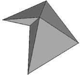
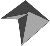
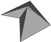
&   Top view Side view       Initial topology Our method Another solution    (a) A Simple example       (b) A more complex example    The problem is illustrated with respect to two pieces of skeleton—a wedge, $A$, and a tabletop, $B$—that are growing relative to each other. Because of the angle of the two front planes of the wedge, the growing wedge eventually grows past the tabletop. The issue that arises at this point is to determine how the wavefronts should continue growing. There are several choices, for example:

Figure 4: 3D skeleton ambiguity.

• The front end of the wedge $A$ is blunted by clipping it with the plane defined by the side of the tabletop.

• The wedge continues growing forward, but is blocked from growing downward by clipping it with the plane defined by the top of the tabletop.

• The wedge suddenly projects into the empty space in front of the table and continues growing out from there.

There are other possibilities, as well. In fact, all three suggestions listed above cause a contradiction or a noncontinuous propagation of the wavefront in certain cases. One poor choice, however, not listed above, is to allow the wedge $A$ to grow through to the other side of $B$ in the case that $A$ reaches the edge of $B$ and moves past the edge. With this 3D skeleton definition it is possible to construct self-contradictory examples with three wedges, $A_{1}$, $A_{2}$, and $A_{3}$, such that $A_{1}$ and $A_{3}$ are on opposite sides of the tabletop and oriented in a way that if $A_{1}$ breaks through $B$, then it blocks $A_{2}$, which in turn does not block $A_{3}$, which in turn breaks through $B$ and prevents $A_{1}$ from breaking through $B$. Likewise, if $A_{1}$ doesn’t break through $B$, then it doesn’t block $A_{2}$, which blocks $A_{3}$, which, in turn doesn’t block $A_{1}$, which breaks through $B$. Thus, we can at least conclude that this rule is an inappropriate choice.

A more general example of the inherent ambiguity of the propagation of the straight skeleton is shown in Figure 4.1(b). The figure shows a vertex of degree 5, and two possible topologies during the propagation. This is the so-called weighted-rooftop problem: Given a base polygon and slopes of walls, all sharing one vertex, determine the topology of the rooftop of the polygon, which does not always have a unique solution. In our definition of the skeleton, we define a consistent method for the initial topology and for establishing topological changes while processing the algorithm’s events, based on the two-dimensional weighted straight skeleton. This method is described in Section 4.3.

4.2 A Combinatorial Lower Bound

We now show that the 3D straight skeleton of an $n$-vertex general simple polyhedron can have asymptotic combinatorial complexity strictly greater than the complexity of the 3D straight skeleton of an orthogonal polyhedron.

Theorem 4.1

The combinatorial complexity of a 3D skeleton for a simple polyhedron is $\Omega(n^{2}\alpha^{2}(n))$ in the worst case, where $\alpha(n)$ is the inverse of the Ackermann function.

Proof

(Sketch) We begin by showing that the cross-section of a set of growing wavefronts can have the same complexity as the upper envelope of a set of line segments in the plane. The construction is illustrated in Figure 5.

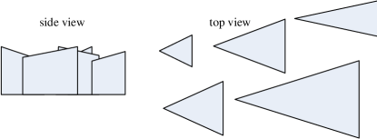
Figure 5: Illustrating 3D skeleton complexity.

The main idea to produce such a cross-section is to set up a sequence of triangular prisms sticking up out of a side of the polyhedron. Construct the set so that the slopes of their top faces matches those of a set of specified line segments and their sides are defined by vertical edges corresponding to the segment endpoints. Define the wedges in sequence with ever sharper points, so that as their wavefronts grow to define the straight skeleton the slower-growing wavefronts in the front are overtaken by the faster ones in the back, until eventually the complexity of the cross-section of the set of growing wavefronts matches that of an upper envelope of line segments. In this case, we can orient the tip of each wedge so that it will be in the visible part of the upper-envelope, which guarantees that the cross-section of the latter portion of the set of growing wavefronts will have the same complexity as the upper envelope of a set of line segments (no matter how the wavefronts are growing in the leading portion of this set of growing wavefronts).

Wiernik and Sharir [25] show that the upper envelope of a set of line segments can have $\Omega(n\alpha(n))$ complexity in the worst case. Thus, the complexity of the cross-section of the set of growing wavefronts in our construction is $\Omega(n\alpha(n))$ in the worst case. Our lower bound for the 3D skeleton follows, then, by having such a set of growing wavefronts attached to the “floor” of a simple polyhedron interact with an orthogonal set of similar growing wavefronts attached to the “ceiling” of a simple polyhedron. This is done by making the direction of growing wavefronts much longer than their cross-sectional length, which implies that as the two sets of wavefronts grow into each other, they produce a number of pieces of straight skeleton that is quadratic in the complexities of the two sets of wavefronts.

4.3 The Algorithm

Figure 6: Changing the initial topology of a vertex of degree greater than 3 (the skeleton is shown in dashed lines): (a) The original polyhedron. Vertex $v$ has degree 5; (b) The cross-section and its weighted straight skeleton. Vertex $v$ becomes three new vertices: $v_{1}$, $v_{2}$, and $v_{3}$; (c) The straight skeleton of the polyhedron. Vertex $v$ spawned three skeletal edges; (d) The propagated polyhedron. Vertices $v_{1},v_{2},v_{3}$ trace their skeletal edges.

Our algorithm for the general case is an event-based simulation of the propagation of the boundary of the polyhedron. Events occur whenever four planes, supporting faces of the polyhedron, meet at the same point. At these points the propagating boundary undergoes topological events. The algorithm for the general case consists of the following steps:

1. Collect all possible initial events.

2. While the event queue is not empty:

   1. Retrieve the next event and check its validity. If the event is not valid, go to Step 2.

   2. Create a vertex at the location of the event and connect to it the vertices participating in the event.

   3. Change the topology of the propagating polyhedron according to the actions taken in Step 2(c). Set the location of the event to the newly-created vertices.

   4. Create new events for newly-created vertices, edges, and faces and their neighbors, if needed.

We next describe the different events and how each type is dealt with. The procedure always terminates since the number of all possible events is bounded from above by the number of combinations of four propagating faces.

Initial Topology.

At the start of the propagation, we need to split each vertex of degree greater than 3 into several vertices of degree 3 (see Figure 6). This is the ambiguous situation discussed earlier; it can have several valid solutions. Our approach is based on cutting the faces surrounding the vertex with one or more planes (any cutting plane intersecting all faces and parallel to none suffices), and finding the weighted straight skeleton of the intersection of these faces with the cutting plane, with the weights determined by the dihedral angles of these faces with the cutting plane, after an infinitesimally-small propagation. The topology of this two-dimensional straight skeleton tells us the connectivity to use subsequently, and always yields a unique valid solution. We establish this method for all types of vertices:

• Convex vertices and spikes. In a convex vertex, all of the edges are on the negative side of its osculating plane. Edges adjacent to convex vertices do not have to be convex. A spike is the opposite of a convex vertex, as all edges are on the positive side of the osculating planes. The topologies of both types can be determined by sectioning, propagating, and finding the weighted straight skeleton.

• Saddle Vertices. In saddle vertices, some of the edges lie on the negative side of the osculating plane, denoted “up” edges, and some on the positive side, denoted “down” edges. We use two sectioning planes. First, we section the edges in the negative side of the plane. Then, we construct their straight skeleton. The section is not a closed polygon, as the intersections of the faces that lead from a “down” edge to an “up” edge, and vice versa, are infinite rays. Every pair of such infinite rays creates a wedge. When computing the weighted straight skeleton of this planar shape, one skeletal vertex will be adjacent to an infinite ray for each such wedge. We call these vertices “portals.” Next, we take each “up”-streak (i.e., a set of “up” edges that are consecutive in a conuterclockwise order around the saddle vertex) and section it by a second plane above the osculating plane. We get a segment-chain, beginning and ending in infinite rays. We calculate the straight skeleton of the segment-chain, resulting in a single vertex of degree 2. Every “up”-streak corresponds to a “down”-wedge, and we connect the last “up” vertex with its corresponding “portal” vertex by an edge. Thus, we get a new fully-connected topology for saddle vertices.

Collecting Events.

In the full version of the paper we describe how events are collected, classified as valid or invalid, and handled by the algorithm. In a nutshell, each processed event arises from interactions of features of the wavefront, and gives rise to potential future events, all of which may be specified by the interaction of four planes. However, a potential event may be found invalid (not corresponding to an actual event in the propagation of the wavefront) already when it is created (since its time stamp is less than that of the current event, or because its geometric location is outside its “region of influence”), or later when it is fetched for processing (if another already-processed event has annulled it). Each valid event results in the creation of features of the skeleton, and in a topological change in the structure of the propagating polyhedron. This part of the algorithm requires a careful case analysis but is conceptually straightforward.

Handling Events.

Propagating vertices are defined as the intersection of propagating planes. Such a vertex is uniquely defined by exactly three planes, which also define the three propagating edges adjacent to the vertex. (When an event creates a vertex of degree greater than 3, we handle it as as in the initial topology—see above.) The topology of the polyhedron remains unchanged during the propagation between events. Figure 7 depicts all possible events:

(a) Edge

(b) Hole

(c) Split

(d) Edge-Split

(e) Vertex

Figure 7: The five types of events. The solid lines are the original edges, and the dashed lines are their locations after the propagation. The dotted arrows show the progression of these edges, up to the time of the event.

1. Edge Event. An edge vanishes as its two endpoints meet, at the meeting point of the four planes around the edge.

2. Hole Event. A reflex vertex (adjacent to three reflex edges, called a “spike”) runs into a face. The three planes adjacent to this vertex meet the plane of the face. After the event, the spike meets the face in a small triangle.

3. Split Event. A ridge vertex (adjacent to one or two reflex edges) runs into an opposite edge. The faces adjacent to the ridge meet the face adjacent to the twin of the split edge. This creates a vertex of degree greater than 3, handled as in the initial topology.

4. Edge-Split event. Two reflex edges cross each other. Every edge is adjacent to two planes.

5. Vertex event. Two ridges sharing a common reflex edge meet. This is a special case of the edge event, as it is the meeting of the endpoints of the reflex edge, but it has different effects, and so it is considered a different event. Vertex events occur when a reflex edge runs twice into a face, and the two endpoints of this edge meet.

A convex polyhedron induces only edge events during propagation, and reduces to a single tetrahedron before vanishing at the simultaneous edge events of the last four edges. A general (nonconvex) polyhedron may split into several connected components, which will be reduced into tetrahedra and similarly vanish. All these events are meeting points of four planes, and other types of events are not accounted for, as they do not occur in general position (e.g., two reflex vertices running into each other), which are meeting points of more than four planes at a location. Note that the propagation of the boundary is “memoryless” in the sense that handling an event does not depend on the history of propagation. Therefore, degenerate events are treated exactly the same as initial vertices of degree greater than 3.

Data Structures.

We use an event queue which holds all possible events sorted by time, and a set of propagating polyhedra, initialized to the input polyhedron (or polyhedra), after the initialization of topology. The used structure is a generalization of the SLAV structure in two dimensions. We provide the details in the full version of the paper.

Running Time.

Let $n$ be the total complexity of the polyhedron, and $k$ the number of events processed by the algorithm. Let $r$ be the number of reflex vertices (or edges) of the polyhedron. In order to collect all the initial events, we iterate over all vertices, faces, and edges of the input polyhedron. Edge events require only looking at each edge’s neighborhood, which can be done in $O(n)$ time. However, finding all hole events requires considering all pairs of a reflex vertex and a face. This takes $O(rn)$ time. Computing a split event is bounded within the edges of the common face, but this can still take $O(rn)$ time, and computing Edge-Split events takes $O(r^{2})$ time.

In the course of the algorithm, we compute and process future events. For a convex polyhedron, only edge events are created, and are easily computed locally in $O(1)$ time per event. However, for a general polyhedron, every edge might be split by any ridge and stabbed by any spike. In addition, new spikes and ridges can be created when events are processed, and they have to be tested against all other vertices, edges, and faces of their propagating connected component. Since $O(1)$ vertices and edges are created in every event, every event can take $O(n)$ time to handle. (The time needed to perform queue operations per a single event, $O(\log{n})$, is comparatively negligible.) The total time needed for processing the events is, thus, $O(kn)$. This is also the total running time of the algorithm.

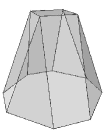
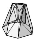
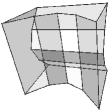
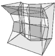
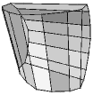
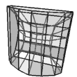
(a)			(b)			(c)
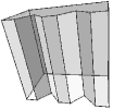
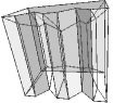
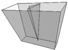
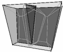
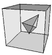
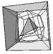
(d)			(e)			(f)
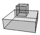
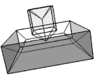
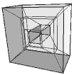
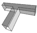
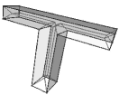
(g)			(h)			(i)

	Object			Skeleton				Time
Object	Vertices	Edges	Facets	Vertices	Edges	Faces	Cells	(Sec.)
General Objects
(a)	12	20	10	8	24	25	10	0.312
(b)	20	30	12	25	60	46	12	0.719
(c)	28	42	16	45	104	74	16	0.567
(d)	20	30	12	16	42	37	12	0.188
(e)	20	18	9(+1)	15	45	56	9	0.250
(f)	12	18	10	21	48	37	10	0.484
Polycubes
(g)	16	24	11	6	21	25	11	0.177
(h)	16	24	11	12	36	33	11	0.146
(i)	16	24	10	12	32	29	10	0.172

(j) Statistics and running times

Figure 8: Sample objects.

5 Experimental Results

We have implemented the algorithm for computing the straight skeleton of a general polyhedron in Visual C++ .NET2005, and experimented with the software on a 3GHz Athlon 64 processor PC with 1GB of RAM. We used the CGAL library to perform basic geometric operations. The source code consists of about 6,500 lines of code. Figure 4.1 shows the straight skeletons of a few simple objects, and the performance of our implementation. (Note that object (e) contains one hole polygon in addition to the 9 facets.)

References

- [1] O. Aichholzer and F. Aurenhammer. Straight skeletons for general polygonal figures in the plane. In Proc. 2nd Ann. Int. Conf. Computing and Combinatorics (COCOON ’96), volume 1090 of Lecture Notes in Computer Science, pages 117–126. Springer-Verlag, 1996.
- [2] O. Aichholzer, F. Aurenhammer, D. Alberts, and B. Gärtner. A novel type of skeleton for polygons. Journal of Universal Computer Science, 1(12):752–761, 1995.
- [3] A. Bagheri and M. Razzazi. Drawing free trees inside simple polygons using polygon skeleton. Computing and Informatics, 23(3):239–254, 2004.
- [4] G. Barequet, M. T. Goodrich, A. Levi-Steiner, and D. Steiner. Contour interpolation by straight skeletons. Graphical Models, 66(4):245–260, 2004.
- [5] E. Bittar, N. Tsingos, and M.-P. Gascuel. Automatic reconstruction of unstructured 3D data: combining a medial axis and implicit surfaces. Computer Graphics Forum, 14(3):457–468, 1995.
- [6] H. Blum. A transformation for extracting new descriptors of shape. In W. Wathen-Dunn, editor, Models for the Perception of Speech and Visual Form, pages 362–380. MIT Press, 1967.
- [7] S.-W. Cheng and A. Vigneron. Motorcycle graphs and straight skeletons. In Proc. 13th Annual ACM-SIAM Symposium on Discrete Algorithms, pages 156–165, 2002.
- [8] L. P. Chew, K. Kedem, M. Sharir, B. Tagansky, and E. Welzl. Voronoi diagrams of lines in 3-space under polyhedral convex distance functions. Journal of Algorithms, 29(2):238–255, 1998.
- [9] T. Culver, J. Keyser, and D. Manocha. Accurate computation of the medial axis of a polyhedron. In Proc. 5th ACM symp. on Solid modeling and applications, pages 179–190, New York, NY, USA, 1999. ACM.
- [10] E. D. Demaine, M. L. Demaine, J. F. Lindy, and D. L. Souvaine. Hinged dissection of polypolyhedra. In Proceedings of the 9th Workshop on Algorithms and Data Structures (WADS 2005), volume 3608 of Lecture Notes in Computer Science, pages 205–217, Waterloo, Ontario, Canada, August 15–17 2005.
- [11] E. D. Demaine, M. L. Demaine, and A. Lubiw. Folding and cutting paper. In Revised Papers from the Japan Conference on Discrete and Computational Geometry (JCDCG’98), volume 1763 of Lecture Notes in Computer Science, pages 104–117. Springer-Verlag, 1998.
- [12] T. K. Dey and W. Zhao. Approximate medial axis as a Voronoi subcomplex. Computer-Aided Design, 36:195–202, 2004.
- [13] D. Eppstein. Dynamic Euclidean minimum spanning trees and extrema of binary functions. Discrete Comput. Geom., 13:111–122, 1995.
- [14] D. Eppstein. Fast hierarchical clustering and other applications of dynamic closest pairs. ACM J. Experimental Algorithmics, 5(1):1–23, 2000.
- [15] D. Eppstein and J. Erickson. Raising roofs, crashing cycles, and playing pool: applications of a data structure for finding pairwise interactions. Discrete & Computational Geometry, 22(4):569–592, 1999.
- [16] M. Foskey, M. C. Lin, and D. Manocha. Efficient computation of a simplified medial axis. Journal of Computing and Information Science in Engineering, 3(4):274–284, 2003.
- [17] J.-H. Haunert and M. Sester. Using the straight skeleton for generalisation in a multiple representation environment. In ICA Worksh. Generalisation and Multiple Representation, 2004.
- [18] M. Held. On computing voronoi diagrams of convex polyhedra by means of wavefront propagation. In Proc. 6th Canadian Conf. on Computational Geometry, pages 128–133, 1994.
- [19] V. Koltun and M. Sharir. 3-dimensional Euclidean Voronoi diagrams of lines with a fixed number of orientations. SIAM Journal on Computing, 32(3):616–642, 2003.
- [20] M. A. Price, C. G. Armstrong, and M. A. Sabin. Hexahedral mesh generation by medial surface subdivision: Part I. Solids with convex edges. International Journal for Numerical Methods in Engineering, 38(19):3335–3359, 1995.
- [21] M. Sharir. Almost tight upper bounds for lower envelopes in higher dimensions. Discrete Comput. Geom., 12:327–345, 1994.
- [22] D. J. Sheehy, C. G. Armstrong, and D. J. Robinson. Shape description by medial surface construction. IEEE Trans. Visualizat. Comput. Graph., 2(1):62–72, Mar. 1996.
- [23] E. C. Sherbrooke, N. M. Patrikalakis, and E. Brisson. An algorithm for the medial axis transform of 3d polyhedral solids. IEEE Trans. Visualizat. Comput. Graph., 2(1):45–61, Mar. 1996.
- [24] M. Tänase and R. C. Veltkamp. Polygon decomposition based on the straight line skeleton. In Proc. 19th Annual ACM Symposium on Computational Geometry, pages 58–67, 2003.
- [25] A. Wiernik and M. Sharir. Planar realizations of nonlinear Davenport-Schinzel sequences by segments. Discrete Comput. Geom., 3:15–47, 1988.