A weak-lensing analysis of the Abell 2163 cluster

Abstract

Aims. We attempt to measure the main physical properties (mass, velocity dispersion, and total luminosity) of the cluster Abell 2163.

Methods. A weak-lensing analysis is applied to a deep, one-square-degree, $r$-band CFHT-Megacam image of the Abell 2163 field. The observed shear is fitted with Single Isothermal Sphere and Navarro-Frenk-White models to obtain the velocity dispersion and the mass, respectively; in addition, aperture densitometry is used to provide a mass estimate at different distances from the cluster centre. The luminosity function is derived, which enables us to estimate the mass/luminosity ratio.

Results. Weak-lensing analyses of this cluster, on smaller scales, have produced results that conflict with each other. The mass and velocity dispersion obtained in the present paper are compared and found to agree well with values computed by other authors from X-ray and spectroscopic data.

1 Introduction

Abell 2163 is a cluster of galaxies at $z$=0.203 of richness class 2 (Abell et al. 1989) and without any central cD galaxy (Fig. 1). It is one of the hottest clusters known so far with an X-ray temperature of 14 keV and an X-ray luminosity of $6\times 10^{45}$ erg s^-1, based on Ginga satellite measurements (Arnaud et al. 1992). Elbaz et al. (1995) used ROSAT/PSPC and GINGA data to map the gas distribution; they showed that the gas extends to at least 4.6 Mpc or 15 core radii and is elongated in the east-west direction; they estimated a total mass $(1.43\pm 0.05)\times 10^{15}M_{\odot}$ $(h=0.5)$ inside that radius, which is 2.6 times higher than the total mass of Coma. The corresponding gas mass fraction, 0.1 $h^{-3/2}$, is typical of rich clusters. The peak of the X-ray emission was found to be close to a bright elliptical galaxy ($\alpha=16^{h}15^{m}49.0^{s}$, $\delta=-06^{\circ}08\arcmin 41\arcsec$), which was confirmed by later X-ray observations (Martini et al. 2007). Two faint gravitational arcs are visible close to this galaxy (Fig. 1); the redshift of the source galaxies is $z_{s}\sim 0.73$ (Miralda-Escude & Babul 1995). The gas velocity dispersion is also very high, $\sigma=1680$ km s^-1 (Arnaud et al. 1994); Martini et al. (2007) derived a velocity dispersion of $\sigma=1381\pm 324$ km/s from spectroscopic data.

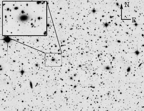
Figure 1: $r-$band image of the Abell 2163 field. The zoomed image shows the bright elliptical galaxy identified as the centre of the cluster from X-ray maps: also visible are the faint gravitational arcs.

ASCA observations of Abell 2163 (Markevitch et al. 1996) measured a dramatic drop in the temperature at large radii: this placed strong constraints on the total mass profile, assumed to follow a simple parametric law (Markevitch et al. 1996). Considerable gas temperature variations in the central 3-4 core radii region were also found. The total mass derived inside $0.5h^{-1}$ Mpc was $(4.3\pm 0.5)\times 10^{14}h^{-1}$ $M_{\odot}$, while inside $1.5h^{-1}$ Mpc it was found to be $(1.07\pm 0.13)\times 10^{15}h^{-1}$ $M_{\odot}$.

Abell 2163 is remarkable also in the radio band: as first reported by Herbig & Birkinshaw (1994), it shows a very extended and powerful radio halo. Feretti et al. (2001) further investigated the radio properties of the cluster. In addition to its size ($\sim 2.9$ Mpc), the halo is slightly elongated in the E-W direction; the same elongation is also seen in the X-ray.

All of this evidence indicates that the cluster is unrelaxed and has experienced a recent or is part of an ongoing merger of two large clusters (Elbaz et al. 1995; Feretti et al. 2004). This was confirmed by Maurogordato et al. (2008), who interpreted the properties of Abell 2163 in terms of a recent merger, in which the main component is positioned in the EW direction and a further northern subcluster (Abell 2163-B) is related to the same complex. They used optical and spectroscopic data to compute, in addition, the virial mass, $M_{\rm vir}=(3.8\pm 0.4)\times 10^{15}$ $M_{\odot}$ and the gas velocity dispersion, $\sim 1400$ km s^-1.

Squires et al. (1997) first performed a weak-lensing analysis of Abell 2163 using a $2048\times 2048$ CCD at the prime focus of the Canada-France Hawaii Telescope (CFHT). They mapped the dark matter distribution up to $7\arcmin$ ($\sim 1h^{-1}$ Mpc); the mass map showed two peaks, one close to the elliptical galaxy, the other at $3\arcmin$ W. The mass obtained by weak lensing alone was a factor of $\sim 2$ lower than that derived from X-ray data: they interpreted the discrepancy in mass measurement as the result of an extension of the mass distribution, beyond the edges of the CCD frame; taking this effect into account, a reasonable agreement is achieved between the mass determined by X-ray and weak lensing. A fit of the shear profile with that expected for a singular isothermal model provided a velocity dispersion measurement of $\sigma=740$ km s^-1, which was lower than the expected value $\sigma>1000$ km s^-1.

Cypriano et al. (2004) completed a weak-lensing analysis of Abell 2163 using FORS1 at the VLT in imaging mode. They measured a higher velocity dispersion of $\sigma=1021\pm 146$ km s^-1. They explained their disagreement with Squires et al. (1997) by the fact that those authors used a bright cut ($V>22$ mag, $I>20.5$ mag) for the selection of background galaxies, whereas they chose $R>23.3$ mag.

Wide-field cameras, such as the ESO Wide-Field Imager (WFI) with a field of view of $34\arcmin\times 33\arcmin$, and the Megacam camera mounted at the CFHT ($\sim 1$ square degree), are particularly well suited for the weak-lensing study of clusters because they enable the clusters to be imaged well beyond their radial extent. We use public archive data of Abell 2163, acquired using the Megacam camera, to complete a revised weak-lensing analysis of this cluster and derive the luminosity function of the cluster galaxies.

This paper is organized as follows. Section 2 describes the data and steps followed in the reduction. The weak-lensing analysis and determination of mass are discussed in Sect. 3. Finally, the cluster luminosity function is derived and the mass to luminosity ratio is computed in Sect. 4.

We adopt $H_{0}=70$ km s^-1 Mpc^-1, $\Omega_{\Lambda}=0.7$, $\Omega_{m}=0.3$, which corresponds to a linear scale of 3.34 kpc/$\arcsec$ at the redshift of Abell 2163.

2 Observations and data reduction

Abell 2163 was observed in 2005 with the Megacam camera at the 3.6m Canada-France Hawaii Telescope in the $r$-band, with a total exposure time of 2.7hr. The prereduced (bias and flat-field corrected) images were retrieved from the Canadian Astronomy Data Centre archive. Before coadding the different exposures, it was necessary to remove the effect of distortions produced by the optics and by the telescope. This was completed using the AstromC package, which is a porting to C++ of the Astrometrix package described in Radovich et al. (2004); we refer the reader to this paper for further details. For each image, an astrometric solution was computed, assuming the USNO-A2 catalog as the astrometric reference and taking into account the positions of the same sources in the other exposures. The absolute accuracy of the astrometric solutions with respect to the USNO-A2 is limited to its nominal accuracy, $\sim 0.3$″; the internal accuracy of the same sources detected in different images is far lower ($\sim 0.01$″), which enables us to optimize the Point Spread Function (PSF) of the final coadded image. AstromC for each exposure computed an offset to the zero point to take into account changes e.g. in the transparency of the atmosphere, relative to one exposure that was taken as reference. Photometric zero points were given already in the header of the images; Table 1 summarizes the photometric parameters. All images were resampled according to the astrometric solution and coadded together using the SWarp software developed by E. Bertin. Finally, catalogs of sources were extracted using SExtractor. Galaxies and stars were selected by the analysis of the $r_{h}$ versus magnitude diagram, where $r_{h}$ is the half-light radius (Fig. 2). The coadded image was inspected to search for regions with spikes and halos around bright stars. Such regions were masked on the image with DS9 and sources inside them were discarded from the catalog. In addition, we did not use the outer part of the image, where the PSF rapidly degraded. The residual available area is 1775 ${\rm arcmin}^{2}$.

Table 1: Photometric calibration terms and magnitude limits computed for point-like sources at different signal to noise ratios in the CFHT-Megacam $r$-band. $A_{r}$ is the average Galactic extinction, for $E(B-V)=0.35$. Megacam zero points are defined so that magnitudes are already on the AB system, and are given here such that the airmass is 0.

Zero point	Color term	Extinction coeff.	$A_{r}$	$m_{\rm AB}(\sigma=3)$	$m_{\rm AB}(\sigma=5)$	$m_{\rm AB}(\sigma=10)$
26.1	0.00$\times$ (g-r)	0.10	0.92	27.0	26.4	25.5

We note that Abell 2163 is located in a region of high Galactic extinction: from the maps by Schlegel et al. (1998), using the dust_getval code we obtain $0.27<\rm{E(B-V)}<0.43$ in the field, with an average value of $\rm{E(B-V)}=0.35$. Such change is significantly higher than the typical uncertainty in $\rm{E(B-V)}$ ($\sim$ 16%, Schlegel et al. 1998): it is therefore more appropriate to correct the magnitude of each galaxy for the extinction value at its position, rather than using the same average value.

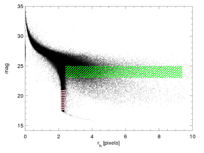
Figure 2: Selection of galaxies used for the lensing analysis (area with oblique lines) and of the stars used for the PSF correction (area with horizontal lines) in the CFHT-Megacam $r$-band image; $r_{h}$ is the half-light radius.

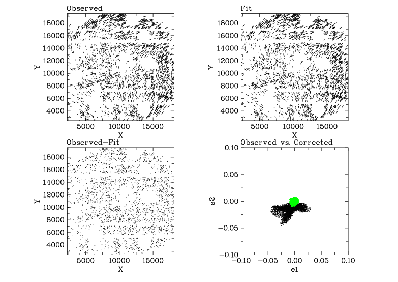
Figure 3: PSF correction: the first three panels show the spatial pattern of the observed, fitted and residual ellipticities of stars: a scaling factor was applied for display purposes; $X$ and $Y$ are the pixel coordinates in the image. The last panel shows the observed versus corrected ellipticities.

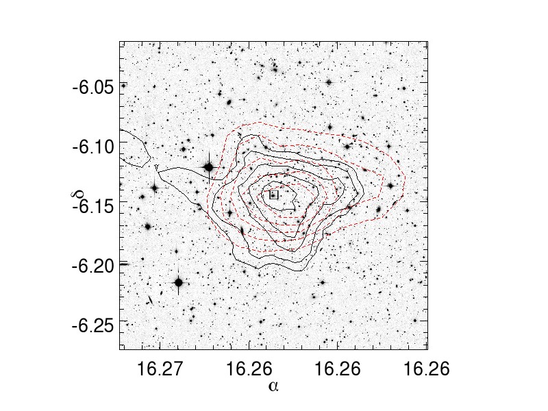
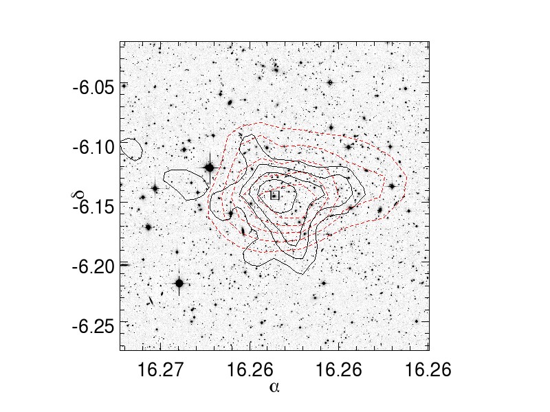
Figure 4: S-maps obtained by aperture densitometry and convolution with up: a Gaussian filter function (size: 5 arcmin); down: the filter function proposed by Schirmer (2004). The contour levels are plotted at $S=(3,4,5,6,7)$, where $S$ is defined in Sec. 3.1.1. The small box indicates the position of the elliptical galaxy with arcs. The dashed contours show for comparison the density distribution of cluster galaxies (see also Maurogordato et al. 2008).

Figure 5: Mass profile obtained by aperture densitometry.

3 Weak-lensing analysis

Weak-lensing relies on the accurate measurement of the average distortion produced by a distribution of matter on the shape of background galaxies. As the distortion is small, the removal of systematic effects, in particular the effect of the PSF both from the telescope and from the atmosphere, is of crucial importance. Most of published weak-lensing results have adopted the so–called KSB approach proposed by Kaiser et al. (1995) and Luppino & Kaiser (1997). We summarize the main points here and refer to e.g. Kaiser et al. (1995), Luppino & Kaiser (1997), and Hoekstra et al. (1998) for more detailed discussions.

In the KSB approach, for each source the following quantities are computed from the moments of the intensity distribution: the observed ellipticity $e$, the smear polarizability $P^{\rm sm}$, and the shear polarizability $P^{\rm sh}$. It is assumed that the PSF can be described as the sum of an isotropic component (simulating the effect of seeing) and an anisotropic part. The intrinsic ellipticity $e_{s}$ of a galaxy is related to its observed one, $e_{\rm obs}$, and to the shear, $\gamma$, by:

$$e_{\rm obs}=e_{s}+P^{\gamma}\gamma+P^{\rm sm}p.$$ (1)

The term $p$ describes the effect of the PSF anisotropy (starred terms indicate that they are derived from measurement of stars):

$$p=e^{*}_{\rm obs}/P^{\rm sm*}.$$ (2)

It is necessary to fit this quantity as it changes with the position in the image, using e.g. a polynomial such that it can be extrapolated to the position of the galaxy. In our case, we find that a polynomial of order 2 describes the data well.

The term $P^{\gamma}$, introduced by Luppino & Kaiser (1997) as the pre–seeing shear polarizability, describes the effect of seeing and is defined to be:

$$P^{\gamma}=P^{\rm sh}-P^{\rm sm}\frac{P^{\rm sh*}}{P^{\rm sm*}}.$$ (3)

As discussed by Hoekstra et al. (1998), the quantity $\frac{P^{\rm sh*}}{P^{\rm sm*}}$ should be computed with the same weight function used for the galaxy to be corrected. For this reason, the first step is to compute its value using weight functions of size drawn from a sequence of bins in the half-light radius $r_{h}$. In many cases, $\frac{P^{\rm sh*}}{P^{\rm sm*}}$ can be assumed to be constant across the image and be computed from the average of the values derived from the stars in the field. We preferred to fit the quantity for the Megacam image, considering its size, as a function in addition of the coordinates (x, y), using a polynomial of order 2. For each galaxy of size $r_{h}$, we then assumed the coefficients computed in the closest bin to finally derive the value of $\frac{P^{\rm sh*}}{P^{\rm sm*}}$.

The implementation of the KSB procedure is completed using a modified version of Nick Kaiser’s IMCAT tools, kindly provided to us by T. Erben (see Hetterscheidt et al. 2007); these tools enable measurement of the quantities relevant to the lensing analysis, starting from catalogs obtained using SExtractor. The package also enables us to separate stars and galaxies in the $r_{h}$-mag space and compute the PSF correction coefficients $P^{\gamma}$, $p$. In addition, we introduced the possibility to fit $P^{\gamma}$ versus the coordinates (x,y), as explained above, and for each galaxy used the values of both $P^{\gamma}$ and $p$ computed in the closest bin of $r_{h}$.

Stars were selected in the range $17.5{\rm mag}<r<21{\rm mag}$, $0.37\arcsec<r_{h}<0.45\arcsec$, providing 2400 stars usable to derive the quantities needed for the PSF correction. As discussed above, these quantities were fitted with a polynomial both for PSF anisotropy and seeing correction: we verified that the behaviour of the PSF across the CCDs enabled a single polinomial function to be used for the entire image (Fig. 3). Galaxies used for shear measurement were selected using the following criteria: $P_{\gamma}>0.25$, $\nu_{\rm max}>5$ , $r_{h}>0.45\arcsec$, $23\rm{mag}<r<25\rm{mag}$, and ellipticities smaller than one. We finally obtained approximately 17000 galaxies, which implied that the average density of galaxies in the catalog was $\sim 8$ galaxies/arcmin².

The uncertainty in ellipticities was computed as in Hoekstra et al. (2000):

$$w=\frac{1}{\sigma_{\gamma}^{2}}=\frac{P^{\gamma^{2}}}{P^{\gamma^{2}}\sigma_{e_{0}}^{2}+\left\langle\Delta e^{2}\right\rangle},$$ (4)

where $\left\langle\Delta e^{2}\right\rangle^{1/2}$ was the uncertainty in the measured ellipticity, $\sigma_{e_{0}}\sim 0.3$ was the typical intrinsic rms of galaxy ellipticities.

Table 2: Best-fit values obtained from the fit of the shear from the NFW model ($c=4.09$). For comparison, the lower rows give the masses computed at the same radii from the best-fit SIS model ($\sigma_{v}=1139_{-56}^{+53}$ km/s, $\theta_{e}=22\arcsec$) and from aperture mass densitometry (A.D.).

	$r_{\rm vir}$	$M_{\rm vir}$	$r_{\rm 200}$	$M_{\rm 200}$	$r_{\rm 500}$	$M_{\rm 500}$	$r_{\rm 2500}$	$M_{\rm 2500}$
	(kpc)	$(10^{14}M_{\odot})$	(kpc)	$(10^{14}M_{\odot})$	(kpc)	$(10^{14}M_{\odot})$	(kpc)	$(10^{14}M_{\odot})$
NFW	$3012\pm 170$	$22\pm 4$	$2362\pm 130$	$18\pm 3$	$1514\pm 90$	$12\pm 2$	$623\pm 40$	$4.2\pm 0.7$
SIS		$18\pm 5$		$14\pm 4$		$9\pm 2$		$4\pm 1$
A.D.		$38\pm 10$		$33\pm 7$		$20\pm 3$		$5.8\pm 0.8$

3.1 Mass derivation

Weak lensing measures the reduced shear $g=\tfrac{\gamma}{(1-\kappa)}$. The convergence $\kappa$ is defined by $\kappa=\Sigma/\Sigma_{\rm crit}$, where $\Sigma$ is the surface mass density and $\Sigma_{\rm crit}$ is the critical surface density:

$$\Sigma_{\rm crit}=\frac{c^{2}}{4\pi G}\frac{D_{s}}{D_{l}D_{ls}}=\frac{c^{2}}{4\pi G}\frac{1}{D_{l}\beta},$$ (5)

$D_{ls}$, $D_{s}$, and $D_{l}$ being the angular distances between lens and source, observer and source, and observer and lens respectively. In the weak lensing approximation, $\kappa\ll 1$, so that $g\sim\gamma$. However, the measured value of $\kappa$ includes an unknown additive constant (the so-called mass-sheet degeneracy): this degeneracy can be solved by assuming either that $\kappa$ vanishes at the borders of the image, or a particular mass profile for which the expected shear is known. Both approaches are used here.

For Abell 2163, $\Sigma_{\rm crit}=9.69\times 10^{13}\beta^{-1}M_{\odot}$ arcmin^-2. In our case, we were unable to assign a redshift to the source galaxies; we however assumed the single-sheet approximation, which implies that the background galaxies lie at the same redshift (King & Schneider 2001). To compute the value of the redshift, we used the publicly-available photometric redshifts obtained by Ilbert et al. (2006) for the VVDS F02 field with Megacam photometric data. We applied the same cuts adopted here for the $r$-band magnitude data and assumed a Gamma probability distribution (Gavazzi et al. 2004):

$$n(z)=z^{a-1}\frac{\exp(-z/z_{s})}{\Gamma(a)z_{s}^{a}},$$ (6)

We found that $a=2.04$ and $z_{s}=0.57$ were the best-fit parameters, and $\rm{Med}(z)=0.98$. We therefore adopted a median redshift of $z\sim 1$, which provided $\left\langle\beta\right\rangle=0.58$.

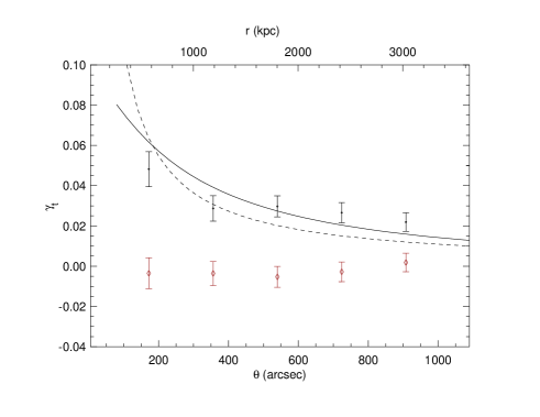
Figure 6: The tangential component of the shear (dark points) is displayed as a function of the distance from the assumed centre of the cluster. The lines show the result of the best-fit to the unbinned data using: a NFW profile with $c_{\rm vir}$ given by Eq. 17 (solid line), and a SIS profile (dashed line). Also shown is the radial component of the shear (diamonds), which is expected to be null in the absence of systematic errors.

3.1.1 Mass aperture maps

Figure 4 displays the S-map introduced by Schirmer et al. (2004), that is:

$$M_{\rm ap}=\frac{\sum_{i}e_{t,i}w_{i}Q(|\theta_{i}-\theta_{0}|)}{\sum_{i}{w_{i}}}$$ (7)

$$\sigma^{2}_{M_{\rm ap}}=\frac{\sum_{i}e^{2}_{t,i}w^{2}_{i}Q^{2}(|\theta_{i}-\theta_{0}|)}{2(\sum_{i}{w_{i}})^{2}},$$ (8)

where $e_{t,i}$ are tangential components of the lensed-galaxy ellipticities computed by considering to be the centre the position in the grid, $w_{i}$ to be the weights defined in Eq. 4, and $Q$ the filter function discussed below. The ratio $S=M_{\rm ap}/\sigma_{M_{\rm ap}}$, defined as the S-statistics by Schirmer et al. (2004), provides a direct estimate of the signal-to-noise ratio of the halo detection.

For the window function, we tested two possible forms: a Gaussian function and a function close to a NFW profile.

The Gaussian window function is defined by:

$$Q(|\theta-\theta_{0}|)=\frac{1}{\pi\theta^{2}_{c}}\exp\left(-\frac{(\theta-\theta_{0})^{2}}{\theta^{2}_{c}}\right),$$ (9)

where $\theta_{0}$ and $\theta_{c}$ are the centre and size of the aperture.

Schirmer (2004) proposed a filter function, whose behaviour is close to that expected from a NFW profile:

$$Q(x)=\left(1+e^{a-bx}+e^{-c+dx}\right)^{-1}\frac{\tanh(x/x_{c})}{\pi\theta_{c}^{2}(x/x_{c})},$$ (10)

where $x=(\theta-\theta_{0})/\theta_{c}$, and we adopted the following parameters: $a=6$, $b=150$, $c=47$, $d=50$, $x_{c}=0.15$ (Hetterscheidt et al. 2005).

In both cases, we found consistently that (i) the peak of the lensing signal was coincident with the position of the bright elliptical galaxy with arcs (BCG hereafter), confirming that this was in fact the centre of the mass distribution as indicated by the X-ray maps; and (ii) the weak-lensing signal is elongated in the E-W direction. A comparison with Fig. 5 and Fig. 9 in Maurogordato et al. (2008) indicates that the mass distribution follows the density distribution of early-type cluster galaxies (the A1 and A2 substructures).

3.1.2 Aperture densitometry

We first estimate the mass profile of the cluster by computing the $\zeta$ statistics (Fahlman et al. 1994; Clowe et al. 1998):

$$\zeta(\theta_{1})=\bar{\kappa}(\theta\leq\theta_{1})-\bar{\kappa}(\theta_{2}<\theta\leq\theta_{\rm max})=2\int^{\theta_{2}}_{\theta_{1}}\left\langle\gamma_{T}\right\rangle d\ln\theta$$ (11)

$$+\frac{2}{1-(\theta_{2}/\theta_{\rm max})^{2}}\int^{\theta_{\rm max}}_{\theta_{2}}\left\langle\gamma_{T}\right\rangle d\ln\theta$$

The quantity $M_{\rm ap}(\theta_{1})=\pi\theta_{1}^{2}\zeta(\theta_{1})\Sigma_{\rm crit}$ provides a lower limit to the mass inside the radius $\theta_{1}$, unless $\bar{\kappa}(\theta_{2},\theta_{\rm max})=0$. This formulation of the $\zeta$ statistics is particularly convenient because it enables a choice of control-annulus size ($\theta_{2}$, $\theta_{\rm max}$) that satisfies this condition reasonably well; in addition, the mass computed inside a given aperture is independent of the mass profile of the cluster (Clowe et al. 1998). Clowe et al. (2004) discussed how the mass estimated by aperture densitometry is affected by asphericity and projected substructures in clusters, as in the case of Abell 2163: they found that the error was less than 5%.

The cluster X-ray emission was detected out to a clustercentric radius of $2.2h^{-1}$ Mpc (Squires et al. 1997), which corresponds to $\sim 900\arcsec$. We took advantage of the large available area and chose $\theta_{2}=1300\arcsec$, $\theta_{\rm max}\sim 1500\arcsec$, which provided $\sim$ 3000 sources in the control annulus. The mass profile is displayed in Fig. 5; the mass values computed at different radii are shown in Table 2.

3.1.3 Parametric models

We consider a Singular Isothermal Sphere (SIS) and a Navarro-Frenk-White (NFW) mass profile, for which the expected shear can be expressed analytically. The fitting of the models is completed by minimizing the log-likelihood function (Schneider et al. 2000):

$$l_{\gamma}=\sum_{1=1}^{N_{\gamma}}{\left[\frac{|\epsilon_{i}-g(\theta_{i})|^{2}}{\sigma^{2}[g(\theta_{i})]}+2\ln\sigma[g(\theta_{i})]\right]},$$ (12)

with $\sigma[g(\theta_{i})]=(1-g(\theta_{i})^{2})\sigma_{e}$.

In the case of a SIS profile, the shear is related to the velocity dispersion $\sigma$ by:

$$\gamma_{t}(\theta)=\frac{2\pi}{\theta}\frac{\sigma^{2}}{c^{2}}\frac{D_{ls}}{D_{s}}=\frac{\theta_{E}}{\theta}$$ (13)

For the Navarro-Frenk-White (NFW) model, the mass profile is (Wright & Brainerd 2000):

$$\rho(r)=\frac{\delta_{c}\rho_{c}}{(r/r_{s})(1+r/r_{s})^{2}},$$ (14)

where $\rho_{c}=3H^{2}(z)/(8\pi G)$ is the critical density of the universe at the cluster redshift; $r_{s}$ is a characteristic radius related to the virial radius by the concentration parameter $c_{\rm vir}=r_{\rm vir}/r_{s}$; $\delta_{c}$ is a characteristic overdensity of the halo:

$$\delta_{c}=\frac{\Delta_{\rm vir}}{3}\frac{c^{3}}{ln(1+c)-c/(1+c)},$$ (15)

$$\Delta_{\rm vir}\sim(18\pi^{2}+82(\Omega_{M}(z)-1)-39(\Omega_{M}(z)-1)^{2})/\Omega_{M}(z).$$

The mass of the halo is:

$$M_{\rm vir}=\frac{4}{3}\pi\Delta_{\rm vir}\rho_{c}r^{3}_{\rm vir}$$ (16)

Bullock et al. (2001) used simulations of clusters to show that the virial mass and the concentration are linked by the relation:

$$c_{\rm vir}=\frac{K}{1+z}\left(\frac{M_{\rm vir}}{M_{\star}}\right)^{\alpha},$$ (17)

with $M_{\star}=1.5\times 10^{13}h^{-1}$ $M_{\odot}$, $K=9$, $\alpha=-0.13$.

Comerford & Natarajan (2007) computed the values of $K$ and $\alpha$ fitting Eq. 17 to the values of virial mass and concentration measured in a sample of 100 clusters; they adopted $M_{\star}=1.3\times 10^{13}h^{-1}$ $M_{\odot}$ and found $K=14.5\pm 6.4$, $\alpha=-0.15\pm 0.13$, which provides values of the concentration which are approximately 1.6 higher than obtained using the relation proposed by Bullock et al. (2001). Given the large uncertainty in the value of $K$, we preferred to adopt the values of Bullock et al. (2001). We used the expression of the shear $\gamma_{t}(r)$ derived by Bartelmann (1996); the minimization in Eq. 12 was completed using the MINUIT package. Figure 6 shows the results of the fit and, for comparison, the binned values of the tangential and radial components of the shear: these are consistent with zero, as expected in the absence of systematic effects. Table 2 shows the masses obtained by model fitting (SIS and NFW), as well as those obtained by aperture mass densitometry at different distances from the BCG, which was assumed to be the centre of the cluster. In addition to $M_{\rm vir}$, the masses obtained for $\rho/\rho_{c}=200,500,2500$ and the corresponding radii $r_{200}$, $r_{500}$ and $r_{2500}$, are also displayed. The value of the virial mass, $M_{\rm vir}=(22\pm 4)\times 10^{14}M_{\odot}$, confirms Abell 2163 as a massive cluster compared to other clusters (Comerford & Natarajan 2007).

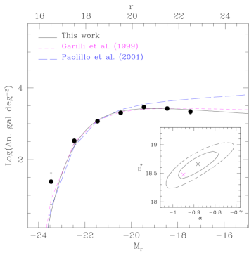
Figure 7: The $r$-band LF of Abell 2163 compared with other determinations in the literature.

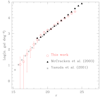
Figure 8: Galaxy counts derived from the control field (empty red circles), compared to literature. The triangles represent the deep counts from the CFH12K-VIRMOS field (McCracken et al. 2003) corrected to the $r_{AB}$ according to Fukugita et al. (1995); the stars mark the counts from the SDSS commissioning data (Yasuda et al. 2001). The error bars of this work take into account only the Poissonian errors ($\sqrt{n}$/area), whereas for the literature counts the errors are not displayed because they are smaller than the point dimensions.

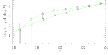
Figure 9: Galaxy counts in the Abell 2163 line of sight (circles) and in the control field (triangles: for display purposes, an offset in $r$ was applied to these points). The lines show the result of the joint fit. The errors bars were computed as described in the text.

Table 3: Best-fit parameters and errors. $a$, $b$, and $c$ describe the shape of galaxy counts, whereas $\alpha$, $m_{\star}$, and $\Phi_{\star}$ describe the shape of the cluster LF. $a$, $b$, $c$, and $\Phi_{\star}$ are in units of $deg^{-2}$. The last two columns show the half width of the 68% and 95% confidence range, with two degrees of freedom.

	Best-fit	68%	95%
$\alpha$	-0.88	0.09	0.15
$m_{\star}$	18.66	0.23	0.40
$\Phi_{\star}/10^{3}$	3.8
$a$	3.19
$b$	0.36
$c$	-0.022

4 Luminosity function

To compute the total $r-$band luminosity of the cluster and hence the $M/L$ ratio, we first derived its luminosity function (LF hereafter). The $r-$band magnitudes were corrected for Galactic reddening as explained in Sect. 2; no k-correction was applied because it is negligible at the redshift of Abell 2163, according to Yasuda et al. (2001).

We defined the cluster region to be the circular area encompassed within $r_{200}$ ($\sim 0.2\deg$, see Table 2) and centred on the BCG. Our control field of galaxies was assumed to be those falling into the outer side (0.36 $\deg^{2}$) of a squared region centered on the BCG of area about 0.25 $\deg^{2}$.

With this choice, we are confident that we minimize the contamination of cluster galaxies and take into account background non-uniformities in the angular scale of the cluster. Figure 8 shows that the $r-$band galaxy counts in the control field are consistent with those found in the literature.

The LF was computed by fitting the galaxy counts in the cluster and control-field areas: we adopted the rigorous approach introduced by Andreon et al. (2005), which allows us to include, at the same time, in the likelihood function to be minimized, the contribution of both background and cluster galaxies. As the model for the counts of the cluster field, we used the sum of a power-law (the background contribution in the cluster area) and a Schechter (1976) function, normalized to the cluster area $\Omega_{cl}$:

$$p_{cl,i}=\Omega_{cl}\Phi_{\star}10^{0.4(\alpha+1)(m_{\star}-m)}\exp(-10^{0.4(m_{\star}-m)})$$ (18)

$$+\Omega_{cl}10^{a+b(m-20)+c(m-20)^{2}}.$$

For the control field, this reduces to the power-law only, normalized to the background area $\Omega_{bkg}$:

$$p_{bkg,i}=\Omega_{bkg}*10^{a+b(m-20)+c(m-20)^{2}},$$ (19)

where $\Phi_{\star}$,$\alpha$, and $m_{\star}$ are the conventional Schechter parameters as usually defined; $a$, $b$, and $c$ describe the shape of the galaxy counts in the reference-field direction; and the value of 20 was chosen for numerical convenience.

Best-fitting parameters (see Table 3) were determined simultaneously by using a conventional routine of minimization on the unbinned distributions. The data were binned for display purpose only in Fig. 9, which shows the binned galaxy counts in the control field (empty triangles) and cluster (empty circles) areas; the joint fit to the unbinned data sets is also overplotted. Error bars are calculated to be $\sqrt{n}/\Omega$. To check the effect of the uncertainty in the position-dependent extinction correction (see Sect. 2), we computed the same parameters in a set of catalogs for which the extinction correction of each galaxy was randomly modified within $\pm$ 15%, the expected uncertainty in $E(B-V)$ (Schlegel et al. 1998): the rms uncertainty in the parameters derived in this way is negligible compared to the uncertainties in the fitting. Figure 7 displays the derived LF compared with selected determinations from the literature, which have been converted to our cosmology.

We compare our LF with Garilli et al. (1999) and Paolillo et al. (2001), which both used data calibrated to the Thuan & Gunn photometric system; according to Fukugita et al. (1995), the offset between this magnitude system and the one used by us is negligible.

Our determination of LF agrees well with Garilli et al. (1999), within the $68\%$ confidence level (see Fig. 7), and has a value of $M_{\star}$ that is consistent with that of Paolillo et al. (2001).

The $r-$band total luminosity was calculated to $L_{\rm tot}=L_{\star}\phi_{\star}\Gamma(2+\alpha)$. The transformation from absolute magnitudes $M_{\star}$ to absolute luminosity $L_{\star}$, in units of solar luminosities, was performed using the solar absolute magnitude, obtained using the color-transformation equation from the Johnson-Morgan-Cousins system to the SDSS system of Fukugita et al. (1995). The errors were estimated by the propagation of the $68\%$-confidence-errors of each parameter. In this way we found that $L_{\rm tot}=(80\pm 2)\times 10^{11}$ $L_{\odot}$, which corresponds to $M_{200}/L_{\rm tot}\sim 230$ ($M_{200}=1.8\times 10^{15}$ $M_{\odot}$, Table 2). Popesso et al. (2007) found a relation between $M_{200}$ and the $r-$band luminosity in 217 clusters selected from the Sloan Digital Sky Survey (see their Eq. 6): according to this relation, the luminosity expected for $M_{200}=1.8\times 10^{15}$ $M_{\odot}$ was $L=(73\pm 10)\times 10^{11}$ $L_{\odot}$, in excellent agreement with the observed value.

5 Conclusions

For the galaxy cluster Abell 2163, we have shown that by the usage of wide-field imaging it is possible to achieve far better agreement than before, between mass and velocity dispersion measured using weak-lensing and those derived for example from X-ray data.

The dispersion velocity here measured, $\sigma=1139^{+52}_{-55}$ km s^-1, agrees well with those derived by X-ray and spectroscopic data, as found by Cypriano et al. (2004), whereas it was underestimated in the previous analysis by Squires et al. (1997).

On the other hand, the comparison with the masses obtained from X-ray measurements (Markevitch et al. 1996) shows that at $r\leavevmode\nobreak\ \sim 2\ {\rm Mpc}$, $M_{X}\sim(1.5\pm 0.2)\times 10^{15}$ $M_{\odot}$ ($h=0.7$); at the same distance, we obtain from the NFW fit (Sect. 3.1.3) $M_{\rm wl}\sim(1.6\pm 0.3)\times 10^{15}$ $M_{\odot}$. We therefore agree with Squires et al. (1997) about the consistency of the mass obtained by weak lensing and X-rays: no correction factor is required in our case due to the larger field of view. We also find a substantial agreement between our estimate of the virial mass, $M_{\rm vir}=(2.2\pm 0.4)\times 10^{15}$ $M_{\odot}$ using the NFW fit, and the value $M_{\rm vir}=(3.8\pm 0.4)\times 10^{15}$ $M_{\odot}$ obtained by Maurogordato et al. (2008) from optical and spectroscopic data; in addition, as noted by these authors, their estimate of the virial mass could be overestimated by 25%. Our weak-lensing analysis also confirms that the mass distribution is extended along the E-W direction, in agreement with that observed in optical, radio and X-ray data (see e.g. Maurogordato et al. 2008).

Finally, the $r-$band total cluster luminosity within $r_{200}$, derived from the luminosity function, gives $L_{\rm tot}/M_{200}=240$. The observed luminosity is in very good agreement with that expected for the mass measured by weak lensing, according to the $L-M$ relation proposed by Popesso et al. (2007).