Structure analysis of interstellar clouds: I. Improving the $\Delta$-variance method

Abstract

Context. The $\Delta$-variance analysis, introduced as a wavelet-based measure for the statistical scaling of structures in astronomical maps, has proven to be an efficient and accurate method of characterising the power spectrum of interstellar turbulence. It has been applied to observed molecular cloud maps and corresponding simulated maps generated from turbulent cloud models. The implementation presently in use, however, has several shortcomings. It does not take into account the different degree of uncertainty of map values for different points in the map, its computation by convolution in spatial coordinates is very time-consuming, and the selection of the wavelet is somewhat arbitrary and does not provide an exact value for the scales traced.

Aims. We propose and test an improved $\Delta$-variance algorithm for two-dimensional data sets, which is applicable to maps with variable error bars and which can be quickly computed in Fourier space. We calibrate the spatial resolution of the $\Delta$-variance spectra.

Methods. The new $\Delta$-variance algorithm is based on an appropriate filtering of the data in Fourier space. It uses a supplementary significance function by which each data point is weighted. This allows us to distinguish the influence of variable noise from the actual small-scale structure in the maps and it helps for dealing with the boundary problem in non-periodic and/or irregularly bounded maps. Applying the method to artificial maps with variable noise shows that we can extend the dynamic range for a reliable determination of the spectral index considerably. We try several wavelets and test their spatial sensitivity using artificial maps with well known structure sizes. Performing the convolution in Fourier space provides a major speed-up of the analysis.

Results. It turns out that different wavelets show different strengths with respect to detecting characteristic structures and spectral indices, i.e. different aspects of map structures. As a reasonable universal compromise for the optimum $\Delta$-variance filter, we propose the Mexican-hat filter with a ratio between the diameters of the core and the annulus of 1.5. When the main focus lies on measuring the spectral index, the French-hat filter with a diameter ratio of about 2.3 is also suitable. In paper II we exploit the strength of the new method by applying it to different astronomical data.

1 Introduction

The interstellar medium is highly turbulent and turbulent motions determine the evolution of interstellar clouds. The turbulent pressure is partially able to support them against gravitational collapse (Klessen et al., 2000); turbulent shocks create and dissolve dense clumps in molecular clouds or even whole clouds (Ballesteros-Paredes et al., 1999), the turbulent mass transport modifies their chemical evolution (Décamp & Le Bourlot, 2002), and the irregular turbulent structure determines their penetration by UV radiation (Zielinsky et al., 2000). Thus, the complex dynamic structure on all scales resulting from turbulence has important implications for many aspects of the astrophysics of the interstellar matter.

Whereas many observations reveal the complexity of the structure of the interstellar medium, most models of interstellar clouds are still based on simple geometrical configurations. A first step towards a better understanding of interstellar turbulence and towards building more realistic models of interstellar clouds is to identify model structures characterised by a limited set of parameters which can be quantified by comparison with observed cloud images. As many aspects of observed interstellar clouds can be described by fractal properties (Combes, 2000), a promising first approach to a parametric description is given by exponents of scaling relations.

Motivated by the similarity of observed interstellar cloud images with the structure of fractional Brownian motion (fBm, see Sect. 2.2.1) fractals, which are characterised by the single number of the exponent of the power spectrum, Stutzki et al. (1998) developed the $\Delta$-variance analysis as a tool to measure the structural scaling behaviour of observed images.

The $\Delta$-variance is a type of averaged wavelet transform that measures the variance in a structure $f(\@vec{r})$ on a given scale $l$ by filtering it by a spherically symmetric down-up-down function of size $l$ (Zielinsky & Stutzki 1999). The $\Delta$-variance analysis was successfully applied to several observational data sets: Stutzki et al. (1998) studied a CO map of the Outer Galaxy, Bensch et al. (2001) investigated a series of nearby star-forming clouds and a number of nested maps in different CO isotopes from the Polaris Flare, Huber (2002) performed a systematic study of a large set of Galactic CO maps, and Sun et al. (2006) analysed maps of the Perseus molecular cloud taken in various tracers and including the analysis of velocity channels. The intensity maps of most clouds resulted in power-law $\Delta$-variance spectra with exponents between 0.5 and 1.3. Mac Low & Ossenkopf (2000) and Ossenkopf (2002) applied the $\Delta$-variance analysis to simulations of interstellar turbulence to compare the scaling behaviour of the simulations with that of observed maps. It became however obvious that, aside from the spectral index, deviations from a power law on particular scales should be studied as well because they provide significant information on the physical processes on these scales. Thus the $\Delta$-variance analysis is to be optimised with respect to its capabilities of the corresponding scale detection.

We propose in this paper a number of improvements to the $\Delta$-variance optimising its sensitivity, its applicability to arbitrary data sets, and the speed of its computation. The critical quantity for the detection of pronounced scales in a structure is the shape of the wavelet filter function. The spherically symmetric down-up-down function introduced by Stutzki et al. (1998) is an obvious first choice. However, other wavelet shapes offer attractive alternatives.

For infinitely extended or for periodic structures the fastest way of numerically calculating the $\Delta$-variance is given by a Fourier transform of the image. However, observed maps typically have a finite size, often even cutting the observed clouds at the map boundary, and Fourier-based methods run into the well known problems of artificial structure being introduced by these edge effects. Bensch et al. (2001) thus implemented the $\Delta$-variance by a numerical treatment in the spatial domain. Calculating a two-dimensional convolution in the spatial domain, however, results in a rather slow computation. An additional complication in observed data comes from the fact that the signal-to-noise ratio is often not uniform across the mapped area. A particular example of maps with strongly variable data reliability are line centroid velocity maps. Here, the accuracy of the centroid velocity always depends on the line intensity. Mac Low & Ossenkopf (2000) have shown that the “traditional $\Delta$-variance analysis may fail in this case. To relieve these problems and concerns, we introduce a supplementary function into the $\Delta$-variance analysis which is used to weight the data points in the spatial map according to their significance. This helps to derive correct contributions of data points with a different signal-to-noise ratio to the structure information on a particular spatial scale and it allows us to calculate the $\Delta$-variance in Fourier space and thus to make use of the numerical advantages of the fast Fourier transform algorithm.

After revising the fundamental properties of the $\Delta$-variance and defining appropriate images to test the method in Sect. 2, we introduce the concepts of the improved $\Delta$-variance including a weighting function in Sect. 3 and optimise it with respect to the wavelet filter function in Sect. 4, where we also verify its performance by extensively testing it against the test structures. A combined test of the optimised filter function and the significance function in the case of noisy data is presented in the Appendix. Sect. 5 summarises our findings providing recommendations for the optimum method and wavelet to use. In a second paper, we test the capability of the new method applying it to simulations of interstellar turbulence and observed molecular line maps exploiting the improved sensitivity to derive general properties of interstellar turbulence.

2 The starting point

2.1 The $\Delta$-variance

The $\Delta$-variance analysis was comprehensively introduced by Stutzki et al. (1998) and Bensch et al. (2001). Here, we only repeat those equations which are essential to understand the extensions proposed in Sects. 3 and 4. Although the $\Delta$-variance can be used in principle for an arbitrary number of dimensions we restrict ourselves to the two-dimensional case, i.e. the analysis of maps or images.

The $\Delta$-variance measures the amount of structure on a given scale $l$ in a map $f(\@vec{r})$ by filtering the map with a spherically symmetric down-up-down function of size $l$ (French-hat filter) and computing the variance of the thus filtered map. It is given by

$$\sigma_{\Delta}^{2}(l)=\left\langle\left(f(\@vec{r})*{\bigodot}_{l}(\@vec{r})\right)^{2}\right\rangle_{\@vec{r}}$$ (1)

where, the average is taken over the area of the map, the symbol $*$ stands for a convolution, and $\bigodot_{l}$ describes the French-hat function defined as

$${\bigodot}_{l}(\@vec{r})={4\over\pi l^{2}}\left\{\begin{array}[]{ll}1&:|\@vec{r}|\leq l/2\\ {-1/8}&:l/2<|\@vec{r}|\leq 3l/2\\ 0&:|\@vec{r}|>3l/2\end{array}\right.$$ (2)

Thus the filter consists of a positive core and a negative annulus where the width of the annulus agrees with the diameter of the core and the absolute values in each of them are inversely proportional to their areas so that they both have an integral weight of unity .

In a more general picture one can consider the filter function as a wavelet composed of a negative and a positive part both normalised to integral values of unity so that the overall filter has a vanishing integral. Using an arbitrary diameter ratio between the annulus and the core $v$ we can write

$${\bigodot}_{l}(\@vec{r}) = \bigodot_{l,{\rm core}}(\@vec{r})-\bigodot_{l,{\rm ann}}(\@vec{r})$$ (3)

$$\bigodot_{l,{\rm core}}(\@vec{r}) = {4\over\pi l^{2}}\left\{\begin{array}[]{ll}1&:|\@vec{r}|\leq l/2\\ 0&:|\@vec{r}|>l/2\end{array}\right.$$ (6)

$$\bigodot_{l,{\rm ann}}(\@vec{r}) = {4\over\pi l^{2}}\left\{\begin{array}[]{ll}{1/(v^{2}-1)}&:l/2<|\@vec{r}|\leq v\times l/2\\ 0&:|\@vec{r}|\leq l/2,|\@vec{r}|>v\times l/2\end{array}\right.$$ (9)

The “traditional” $\Delta$-variance filter is reproduced for a diameter ratio $v=3$. We come back to discussing the choice of $v$ in Sect. 4.

Because the average distance between two points in the core and the annulus of the filter is close to the length $l$ (see Sect. 4.2), the convolved map only retains variations on that scale whereas variations on smaller and larger scales are suppressed. The $\Delta$-variance as the variance of the convolved map thus measures the amount of structural variation on the scale $l$. Plotting the $\Delta$-variance as a function of the filter size $l$ then provides a spectrum showing the relative amount of structure in a given map as a function of the structure size.

The filter convolution and computation of the $\Delta$-variance can be easily performed in Fourier space where they are reduced to a simple multiplication and integration. This directly relates the $\Delta$-variance to the power spectrum. If $P(|\@vec{k}|)$ is the radially averaged power spectrum of the structure $f(\@vec{r})$, the $\Delta$-variance is given by

$$\sigma_{\Delta}^{2}(l)=2\pi\;\int_{0}^{\infty}P(|\@vec{k}|)\;\left|\tilde{\bigodot}_{l}(|\@vec{k}|)\right|^{2}|\@vec{k}|\;d|\@vec{k}|$$ (10)

where $\tilde{\bigodot}_{l}$ is the Fourier transform of the filter function with the size $l$ and $\@vec{k}$ denotes the spatial frequency or wavenumber. If the power spectrum is given by a power law, $P(|\@vec{k}|)\propto|\@vec{k}|^{-\zeta}$, the $\Delta$-variance also follows a power law $\sigma_{\Delta}^{2}\propto l^{\alpha}$ with $\alpha={\zeta-2}$ within the exponential range $0\leq\zeta<6$ (Stutzki et al., 1998).

Thus, the $\Delta$-variance shows in principle only information that is also contained in the power spectrum. The main advantage of the $\Delta$-variance method compared to the direct computation of the power spectrum results from the smooth filter shape which provides a very robust way for an angular average, insensitivity to singular variations, and independence of gridding and finite map size effects. It provides a good separation of different effects based on their characteristic scale, e.g. a clear distinction between observational noise, structure blurring by the finite telescope beam, and the internal scaling of the astrophysical source. A detailed computation of the influence of finite map sizes and telescope blurring was provided by Bensch et al. (2001).

However, when applying Eq. (10) to compute the $\Delta$-variance it inherits a main drawback from the power spectrum – it implicitly assumes a periodic continuation in the Fourier transform although most astrophysical observations show no periodicity. Sect. 3 thus deals with the implications of this assumption and possible ways to overcome the resulting limitations.

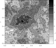
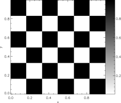
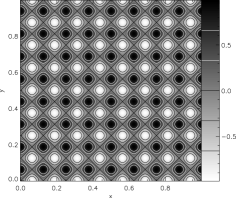
Figure 1: Examples of periodic data sets used to test the $\Delta$-variance algorithm. The fBm structure on the left is characterised by a spectral index $\zeta=3.0$. The chess board has a characteristic structure size of about 0.13. The sine wave field on the right consists of a single Fourier component at $k=8$, the corresponding characteristic distance is $0.09$.

2.2 Test data sets

In order to test how the $\Delta$-variance reproduces specific structural characteristics, we have constructed a series of artificial data sets with known characteristics. They were either chosen to reproduce the typical self-similar scaling behaviour measured in many astrophysical observations (Combes, 2000) or to contain pronounced artificial structures with a well known size scale which should be clearly detected in the $\Delta$-variance spectrum. All test data sets were generated with an intrinsic resolution of $128\times 128$ pixels.

2.2.1 Periodic data

As a simple test bed where boundary effects play no role we started with three types of periodic maps. The first type is provided by the fractal structures of fractional Brownian motion (fBm) as used by Bensch et al. (2001). fBm structures are defined by a power-law power spectrum $P(|\@vec{k}|)\propto|\@vec{k}|^{-\zeta}$ and random phases in Fourier space. We created fBms by the Fourier transform of a Hermitian field with amplitudes following the power spectral index $\zeta$ and random phases. This procedure guarantees real values and periodic maps. The structure analysis in terms of the $\Delta$-variance should recover the power spectral index of the fBm structure measuring a slope $\alpha=\zeta-2$ for this data set.

As periodic structure with a pronounced size scale we use chess board like patterns where the number of fields on the board is varied to change the size of the structures in the map relative to the map size. Because the single chess fields are the only structure in this data set, their size should appear as prominent peak in the $\Delta$-variance spectrum. This data set gives a sharp definition of the characteristic length scale in the spatial domain but contains a high contribution of high frequency modes in the spatial frequency domain due to the sharp edges of each field. Thus we have added as a third type of test maps data fields provided by a single Fourier component in both directions, i.e. the superposition of two orthogonal sine waves with the same period, $f(\@vec{r})=\cos(2\pi kx)+\sin(2\pi ky)$. In the case of a wavenumber $k=1$ it can be regarded as an fBm with $\zeta\rightarrow\infty$. The scale of the characteristic variation should be clearly detected but in contrast to the power spectrum we do not expect a single sharp maximum in the $\Delta$-variance spectrum, because the Fourier transform of the $\Delta$-variance filter is a Bessel function with pronounced side lobes.

The test data sets are all characterised by one free parameter. For the fBms this is the spectral index $\beta$. For the chess board pattern and the sine wave field it is the size of the characteristic structure or the dominant wavenumber, respectively. Examples of the test data sets are shown in Fig. 1. The fBm structure used here is characterised by a spectral index $\zeta=3.0$ and a total variance of 1. The chess board example shows characteristic structure lengths between 0 and 0.24. Its average size, integrated over all possible angles is 0.13. The sine wave field shown here is characterised by a wavenumber $k=8$ leading to a length of 0.09 for the maximum variation.

2.2.2 Non-periodic data

As real astrophysical data are hardly periodic, tests for the treatment of boundary effects have to be performed on non-periodic data. We use two types of data sets to study these effects.

First we select subsets of larger (periodic) fBm structures in the same way as introduced by Bensch et al. (2001). The subsets cover one quarter in length, i.e. $1/16$ in area, of the periodic fBm field so that they should hardly retain any information about the large-scale periodicity. As the subsets are randomly chosen they typically show sharp discontinuities at the edges. This seems to exclude Fourier based methods for the analysis. In Sect. 3.1 we show, however, that the $\Delta$-variance analysis can be extended to account for the discontinuities. Although it is not guaranteed that a subset has the same spectral index as the whole fBm structure we will judge the value of the $\Delta$-variance analysis based on the agreement of the determined spectral index with the original fBm index because this approach reflects the typical observational strategy that high resolution observations are restricted to small parts of a molecular cloud but they are used to derive the general scaling behaviour of the cloud (see e.g. the IRAM keyproject “Small-scale structure of pre-star-forming regions”, Falgarone et al., 1998).

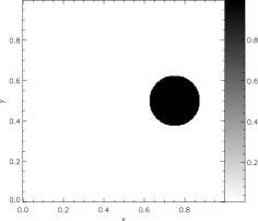
Figure 2: Example of a filled circle structure used to test the $\Delta$-variance algorithm. The diameter of the circle is 0.25.

As second non-periodic structure we use a filled circle on an otherwise empty map. The dominant scale is the size of the circle but as the $\Delta$-variance also measures the size of the “empty” surroundings of the circle we expect considerable contributions from this area to the spectrum at large lags. By adjusting the position of the circle with respect to the map boundaries we can test the robustness of the edge treatment in the non-periodic algorithm (in a periodic treatment the $\Delta$-variance is independent of the position of the circle). The main free parameter of this structure is the diameter $d$ of the circle. The average circle scale is given by $\pi/4d$. We have not scanned the distance to the map boundary as an additional free parameter, but only performed a few tests for circles shifted by a integer multiples of the full diameter relative to the centre. An example with a circle diameter of 0.25 is shown in Fig. 2.

3 Weighting in Fourier space

3.1 Edge treatment

In the introduction of the $\Delta$-variance by Stutzki et al. (1998) we made extensive use of the Fourier transform, applying Eq. (10) to convolve the astrophysical image with the $\Delta$-variance filter. With the Fourier transform implicitly assuming data periodicity, we introduce, however, steps at the edges of a map if the intensity does not show the same value on both sides. Because step functions contain contributions at all spatial frequencies they distort the $\Delta$-variance spectrum of the original structure. Bensch et al. (2001) have shown that this effect can lead to considerable errors for most astrophysical structures, where a periodic continuation is not possible.

The solution proposed there with the POINT and PIX algorithms was a modification of the filter function when applied close to the boundaries of the maps. The filter is truncated so that it never stretches beyond the map edges. To guarantee that the core and the annulus are still normalised to unity for the truncated filter, both parts are multiplied with correction factors depending on the remaining filter size. This edge treatment has, however, the disadvantage that different parts of a map are convolved with a different filter function so that the computation of the $\Delta$-variance by Fourier transform via Eq. (10) is no longer possible. In Bensch et al. (2001) we thus concluded that the $\Delta$-variance should be rather computed in ordinary space. This approach is, however, slow compared to the computation in Fourier space (several hours instead of a few seconds for maps containing more than about 100$\times$100 pixels).

Here, we introduce a method that combines the improved edge treatment with a computation in Fourier space. It is fast and does not introduce artificial high-frequency contributions by periodically wrapping discontinuities at the map edges. To obtain this behaviour the method is set up to fulfil three conditions: i) In the convolution a fixed filter function is to be used so that the convolution can be computed by multiplication in Fourier space. ii) To avoid effects of periodic edge-wrapping, the filter contributions beyond the edges of the map have to be truncated. iii) The normalisation of the filter discussed in Sect. 2.1 has to be fulfilled at each point.

These apparently conflicting requirements can be met using two simple ideas. The truncation of the filter is substituted by a zero-padding of data and the corresponding error in the filter normalisation is corrected by weighting factors for the two filter contributions computed as a function of the coordinates in the map.

Instead of truncating the filter when it extends beyond the map edges we increase the map by zero-padding beyond the edges up to the maximum filter size used. Then the extended map can be convolved with a fixed filter function, only providing zero contributions from outside the original map. In this way no points from other periodically wrapped parts of the image may then fall into the filter centred at any map position. The error in the normalisation of the filter introduced by this substitution can be computed from the convolution of the filter with an auxiliary map $w(\@vec{r})$, which has a value 1 inside the range of valid data and 0 in the zero-padded region. Because the $\Delta$-variance filter $\bigodot_{l}$ has to fulfil the two normalisation conditions for the core and the annulus (see Eq. 9)

$$\sum_{\rm map}\bigodot_{\rm{\it l},core}(\@vec{r})=\sum_{\rm map}\bigodot_{\rm{\it l},ann}(\@vec{r})=1$$ (11)

it has to be split into the positive and negative filter parts for the computation of the normalisation errors. The sums extend over the map of valid data. In total four convolution integrals need to be evaluated to compute the $\Delta$-variance

$$G_{l,{\rm core}}(\@vec{r}) = f_{\rm padded}(\@vec{r})*\bigodot_{l,{\rm core}}(\@vec{r^{\prime}})$$

$$G_{l,{\rm ann}}(\@vec{r}) = f_{\rm padded}(\@vec{r})*\bigodot_{l,{\rm ann}}(\@vec{r^{\prime}})$$

$$W_{l,{\rm core}}(\@vec{r}) = w(\@vec{r})*\bigodot_{l,{\rm core}}(\@vec{r^{\prime}})$$

$$W_{l,{\rm ann}}(\@vec{r}) = w(\@vec{r})*\bigodot_{l,{\rm ann}}(\@vec{r^{\prime}})$$ (12)

where $f_{\rm padded}$ stands for the map with the additional zero-padded boundary region. As we use fixed filter functions and all involved functions vanish at the map edges, the convolution integrals can be easily computed in Fourier space involving a fast Fourier transform and a map multiplication. Although the map treated in this way is larger than the original map by up to a factor three in each direction, the Fourier transform using an algorithm like FFTW, which can work on arbitrary map sizes, is still considerably faster than any convolution in ordinary space.

The full map convolved with the $\Delta$-variance filter truncated at the map edges is then

$$F_{\rm l}(\@vec{r})={G_{\rm{\it l},core}(\@vec{r})\over W_{\rm{\it l},core}(\@vec{r})}-{G_{\rm{\it l},ann}(\@vec{r})\over W_{\rm{\it l},ann}(\@vec{r})}$$ (13)

It is only defined where the normalisation parameters $W_{\rm{\it l},core}$ and $W_{\rm{\it l},ann}$ are both different from zero.

In the computation of the $\Delta$-variance spectrum one has to take into account the reduced significance of the data values in the convolved maps produced by the fact that the applied filter becomes more and more distorted relative to the optimum filter when it is truncated. Using the normalisation parameters of the truncated filters as a measure for their significance one can add a significance weighting to the $\Delta$-variance analysis. We define the $\Delta$-variance no longer as the variance of the convolved map but weight the map points by the significance of the filter applied to compute the value at each point when computing the variance

$$\sigma_{\Delta}^{2}(l)={\sum_{\rm map}(F_{\rm l}(\@vec{r})-\langle F_{\rm l}\rangle)^{2}W_{\rm{\it l},tot}(\@vec{r})\over\sum_{\rm map}W_{\rm{\it l},tot}(\@vec{r})}$$ (14)

with

$$W_{\rm{\it l},tot}(\@vec{r})=W_{\rm{\it l},core}(\@vec{r})W_{\rm{\it l},ann}(\@vec{r})$$ (15)

The sum covers the whole (extended) convolved data field. The definition of the significance function as the product of both normalisation factors is somewhat arbitrary but reproduces the desired behaviour that changes in the positive and negative part of the filter contribute equally. We have tested different powers of the product but found the best agreement with the theoretical behaviour in fBm data sets for an exponent of just unity.

Figure 3: $\Delta$-variance spectra computed with three different types of the edge treatment for one periodic fBm structure (upper plot) and one non-periodic subset from a fBm structure (lower plot). The fBms are characterised by a spectral index $\zeta=3.0$ so that the $\Delta$-variance should show a slope $\alpha=1.0$. The measured slopes are indicated for each graph in the plot.

Figure 3 demonstrates the effect of the edge treatment in the example of an fBm structure which is periodic and for a non-periodic sub-map from a larger fBm structure. We have used three different ways to compute the $\Delta$-variance. First we assume that the maps are periodic, neglecting all wrap-around effects. For the periodic fBm this is, of course, the best assumption which should reproduce exactly the properties of the power spectrum used to generate the fBm. It is, however, rarely useful when dealing with observed data as they are in general not periodic. The second approach creates periodicity by mirroring the map along both axes as discussed by Stutzki et al. (1998) so that a larger periodic map is produced and wrap-around effects can be neglected. This approach, however, still results in discontinuities in the first derivatives at the mirror axes. The third approach uses the truncated filter as described above.

For the periodic fBm structure we find a very close agreement of the $\Delta$-variance using the truncated filter with the theoretical value given by a slope $\alpha=1$. The mirror continuation results in an apparent reduction of the amount of large-scale structures in the map as they are partially assigned to larger modes only present in the map extended by mirroring. Thus the $\Delta$-variance slope is systematically underestimated. For the non-periodic structure, the assumption of periodicity results in strong deviations from the power-law behaviour on small scales due to artificial high-frequency contributions from the edges. The mirroring shows again an underestimate of the power spectral index on large scales, and only the use of the truncated filters results in a good reproduction of the expected value for the slope.

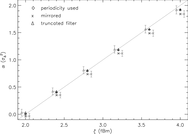
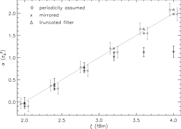
Figure 4: Average and standard deviation of the spectral indices of the $\Delta$-variance spectra determined for a set of fBm structures (upper plot) and for a set of sub-maps from fBm structures (lower plot) depending on the spectral index of the fBms. All spectra are computed at the same power spectral indices $\zeta=2.0,2.4,2.8,3.2,3.6,$ and 4.0, but for a better visibility, the standard deviations for the truncated filter and for the mirror continuation are displaced in the plot relative to these values. In the case of the periodic analysis of the fBm maps the error bars giving the standard deviation of the statistical samples are practically zero. The dotted line indicates the theoretical index for infinitely large fBm structures $\alpha=\zeta-2$.

In Fig. 3 we plot the results obtained just for one realization of an fBm and for one sub-map from a large fBm. But the exact shape of the computed $\Delta$-variance spectra can depend on the distribution of the random phases within the fBm and it will certainly depend on the selection of the sub-map within an fBm. Thus we have repeated the computation for a set of maps in Fig. 4. Analogously to the statistical treatment by Bensch et al. (2001) we vary the spectral index of the fBm structures and chose randomly 30 different fBms or fBm sub-maps and determine their $\Delta$-variance spectra. We do not display all spectra, but only the resulting distribution of slopes $\alpha$. The Fig. shows the average $\Delta$-variance slope and the spread of measured slopes as a function of the spectral index $\zeta$ using the three different edge treatments. All slopes are computed from a power fit covering the full data range plotted in Fig. 3. An optimum treatment should reproduce the relation $\alpha=\zeta-2$ indicated by the dotted line in Fig. 4.

For the periodic fBms we find that the $\Delta$-variance spectra from the truncated filter show about the same spectral indices as the periodic treatment. The error bars in the periodic treatment are zero because the $\Delta$-variance spectrum is independent of the exact phase distribution and thus identical for each map of the sample. The standard deviation of the slopes in the truncated-filter treatment is always about 0.08 here. The $\Delta$-variance spectrum underestimates the power spectral index by 0.03 at $\zeta=3.6$ and by 0.08 at $\zeta=4$ because the theoretical value is only reached for infinitely large maps and the deviations grow when approaching the asymptotic limit of $\alpha=4$ (see Stutzki et al. 1998). The $\Delta$-variance spectrum computed for the mirror-continuation of the map always underestimates the spectral index by about 0.1.

In the case of non-periodic fBm sub-structures the periodicity assumption clearly fails. With this approach the measured slope saturates at about $\alpha=1.1$. The use of the simple $\Delta$-variance without filter truncation or mirror continuation provides wrong results at power spectral indices above about $\zeta=2.9$. This is due to unavoidable discontinuities at the submap edges which result in high-frequency contributions in the periodic treatment resulting in too shallow $\Delta$-variance spectra. In contrast, both the mirror-continuation and the filter truncation provide a reasonable measure for the actual map structure for all spectral indices. Both methods are hardly affected by the discontinuities at the sub-map edges. The mirror-continuation always underestimates the spectral index by about 0.1 (except at $\zeta=4.0$). The filter truncation method reveals the correct spectral index for $\zeta\leq 3.0$ and overestimates it by 0.05 at $\zeta=4.0$. Regarding the typical error bars of 0.15, the systematic errors are, however, lower than the scatter between different fBm realizations with the same spectral index.

The same tests were repeated for map sizes ranging from $32^{2}$ to $256^{2}$ pixels. In agreement with the studies by Bensch et al. (2001) we found no systematic changes in the $\Delta$-variance slopes exceeding 0.03 when changing the map size but an increase of the error bars from 0.15 at map sizes of $128^{2}$ to 0.25 at a size of $32^{2}$. This higher uncertainty for smaller maps prevents any significant conclusion from maps spanning less than $\approx 30$ pixels.

Figure 5: $\Delta$-variance spectra for the filled-circle map where the circle has a diameter of 1/8 of the map size and is shifted by three diameters from the centre of the map. The values $\hat{l}$ indicate the lag of the measured peak in the spectrum.

To demonstrate the influence of the edge treatment on the $\Delta$-variance spectrum of an object with a pronounced size scale we show in Fig. 5 the spectra computed for the map containing the filled circle with a diameter of 1/8 of the map size. The peak of the $\Delta$-variance spectra at 0.11 falls below the circle diameter of 0.125 but slightly above the average distance between two points on the rim of the circle which is about 0.10. The somewhat higher value is probably due to the contributions from the “empty” environment of the circle at large lags, also resulting in a decay of the $\Delta$-variance spectra at large lags which is shallower than the $l^{-2}$-characteristics of uncorrelated structures.. These contributions are dispersed over a relatively wide range of scales corresponding to the different distances to the map boundary in a non-periodic treatment and to the distances to the next circle in a periodic interpretation of this structure. As these variations are mainly assigned to lags exceeding the map size in the periodic treatment, the two curves for the periodic treatment show somewhat lower $\Delta$-variance values within the map than the filter truncation method where the “empty” region is constrained by the map size. Nevertheless, the total differences between $\Delta$-variance spectra using the different edge treatment methods are relatively small, so that either method seems to be justified for this case.

3.2 Generalisation for data with varying reliability

The concept of weighting the $\Delta$-variance computation by different filter significance values can be generalised to deal with data, where the data points in a map are as well characterised by a variable data reliability. This applies e.g. to maps where not all points are observed with the same integration time so that they show a different noise level. The inverse noise RMS is an indicator for the significance of the data at different points. Many other observational effects may lead to a similar variation in the data reliability across the map. As long as the reliability can be expressed as a significance number $w_{\rm data}(\@vec{r})$ between 0 and 1 all such maps may be analysed within the concept outlined here. The same equations as discussed in the filter truncation are to be applied, but the auxiliary weight map $w(\@vec{\@vec{r}})$ does no longer consist of the values 1 inside and 0 outside of the original map. It rather contains the significance values $w_{\rm data}(\@vec{r})$ ranging continuously from 0 to 1. The weighting factors in the $\Delta$-variance computation $W_{\rm{\it l},tot}(\@vec{r})$ then contain the integrated significance of the filter-convolved data at each point.

With this generalised concept, the $\Delta$-variance analysis can be applied to arbitrary two-dimensional data sets. They must be projected onto some regular grid but they do not need to contain regular boundaries as the corresponding “empty” grid points only have to be marked with a zero significance. Varying noise or other changes in the data reliability can be expressed in the significance function $w_{\rm data}(\@vec{r})$ which has to be constructed for each data set. The only remaining requirement for the applicability of the $\Delta$-variance is the sufficiently large spatial dynamic range in the data. The criterion of at least 30 pixels in each direction for reasonable error bars of the $\Delta$-variance spectrum discussed above has to be extended in the case of a low data significance. In the appendix we present measurements of the dynamic range over which the slope of fBms can be reliably determined in the case of noisy data. We find as a rule of thumb that the minimum map size has to be increased by one over the average data significance. In paper II we will apply the $\Delta$-variance analysis to observed data with irregular boundaries and a spatially varying significance.

4 Filter optimisation

4.1 The $\Delta$-variance filter function

All examples given above were computed with the fixed filter function of a French hat with a diameter ratio between the annulus and the core $v=3$. An obvious question is whether we can improve on the $\Delta$-variance by using a different diameter ratio and/or a different filter function. Due to its discontinuity in the normal space the French hat has high frequency lobes in Fourier space. Alternative approaches should use smoother functions in ordinary space to obtain a better confinement in Fourier space. As a smooth example we implemented a “Mexican hat” consisting of two Gaussian functions:

$$\bigodot_{l,{\rm core}}(\@vec{r}) = {4\over\pi l^{2}}\exp\left(\@vec{r}^{2}\over(l/2)^{2}\right)$$ (16)

$$\bigodot_{l,{\rm ann}}(\@vec{r}) = {4\over\pi l^{2}(v^{2}-1)}\left[\exp\left(\@vec{r}^{2}\over(vl/2)^{2}\right)-\exp\left(\@vec{r}^{2}\over(l/2)^{2}\right)\right]$$

where $l$ is the size of the filter and $v$ is the diameter ratio between the annulus and the core of the filter as defined in Sect. 2.1. The choice of the Gaussians guarantees that the filter gives the best simultaneous confinement in ordinary space and in Fourier space not showing any side lobes in either of them.

As the opposite extreme we have also tested a filter measuring the difference between one point in the map and all points displaced by the sharp distance $l$ relative to this pixel. The corresponding $\Delta$-variance then measures basically the structure function of the map (see e.g. Miesch & Bally, 1994; Frick et al., 2001). However, because those tests only confirmed the results from Ossenkopf & Mac Low (2002) and Frick et al. (2001) that the structure function is relatively insensitive to distortions of the power spectrum on particular scales we excluded this filter from the following studies.

Thus, we restrict ourselves here to the Mexican- and the French-hat filter, where we vary in both cases the diameter ratio $v$. In this way we test both the influence of the general filter shape and of the ratio between core and annulus for each filter on the computed $\Delta$-variance spectra.

4.2 The effective filter length

Taking into account the finite width of the core and the annulus of both filter functions it is not obvious on which scale variations are actually measured when using a filter with size $l$. Here, we compute this scale based on the geometrical properties of the filter.

In the French-hat filter we measure the average distance between a point in the core and a point in the annulus, providing the average scale on which a structure variation in the map should be measured. For the Mexican-hat filter, the computation of the average distance includes the additional weighting of each distance by the product of the positive and negative filter values. This reflects the effect of the convolution of a map with this filter.

Figure 6: Factor translating the filter core diameter $l$ into the average distance measured by the filter as a function of the diameter ratio between annulus and core of the filter. The average distance is computed by a double integral over the core and the annulus of the filter.

Figure 6 shows the resulting effective filter length relative to the filter size $l$ as a function of the diameter ratio $v$ for the French and the Mexican hat. The length scale traced by the filters is approximately a linear function of the diameter ratio between the core and the annulus of the filter. Using a least-square fit we obtain the coefficients

$${l_{\rm eff}\over l}=\left\{\displaystyle 0.29v+0.26\quad{\rm for\;the\;French\;hat}\hfill\atop\displaystyle 0.41v+0.46\quad{\rm for\;the\;Mexican\;hat.}\hfill\right.$$ (17)

The original $\Delta$-variance definition using a French hat with $v=3$ gives an effective length of 1.12 times the core diameter $l$. Thus all scales computed previously with that filter should be shifted by the factor 1.12. This is only a small correction, not changing the conclusions in any of the papers that have used the $\Delta$-variance so far. In all plots shown in this paper, we use the effective length as the lag of the $\Delta$-variance to allow a direct comparison of the spectra independent of the filter used.

4.3 Filter evaluation

The optimum filter to be used in the $\Delta$-variance analysis has to fulfil two criteria: the correct detection of pronounced size scales in the maps and the exact determination of the scaling exponents of the contained structures.

4.3.1 Scale detection

In the detection of pronounced scales the maximum of the $\Delta$-variance spectrum should fall onto the correct lag corresponding to the structure size. Moreover, the signature of the pronounced scale in the $\Delta$-variance spectrum should be as sharp as possible with a high contrast relative to other scales. As test images we used the chess board field, the sine wave field, and the filled circle field.

Figure 7: $\Delta$-variance spectra computed for the sine wave field with a wavenumber $k=8$. The filter truncation is applied in both cases for the edge treatment. The peak scale is given as $\hat{l}$, the logarithm of the ratio between upper and lower lag where the $\Delta$-variance has dropped to $1/2$ of the peak value is given as $w$.

To illustrate the behaviour we plot the results for the sine wave field. Fig. 7 shows the $\Delta$-variance spectra measured for a field with $k=8$ by the French and the Mexican-hat filters. In both cases the filter truncation method is used. The dominant scale is detected as a peak in the $\Delta$-variance spectra, the peak position at about 0.07 is somewhat lower than the scale of the maximum variation $1/(k\sqrt{2})=0.088$. We found this small shift by about 20 % in all spectra. When using the effective filter length, the peak position is very constant independent of the filter type and its diameter ratio.

On scales above the peak, the spectra obtained for the two filters deviate considerably. The French-hat filter produces ripples at large lags. From the positions of these ripples we find that they reflect the side lobes of the Bessel function, representing the Fourier transform of the French-hat filter. This must not be misinterpreted as a detection of large-scale structure in the map. The side lobes detect the single Fourier amplitude from $k=8$ also at other effective filter sizes. This can be seen when changing the diameter ratio $v$ in the filter. The peak remains at the same position but the ripples in the $\Delta$-variance spectrum move corresponding to the changes in the side lobes of the Bessel function. Decreasing $v$ relative to the value of 3.0 results in a steeper decay above the peak and an increased number of ripples at large lags. When reducing the diameter ratio $v$ for the Mexican-hat filter the decay above the peak also steepens and we obtain some flattening at the largest lags in the map. In general we can either achieve the sharp peak and the artificial structures at large lags by the French-hat filter or the broader peak without ripples by means of the Mexican hat.

Because the field is periodic we can also apply the periodic continuation method here. The equivalent figure shows the same shape of the peak but more pronounced ripples with deeper minima on large scales for the French hat filter and a somewhat steeper decay for the Mexican hat. In this case the $\Delta$-variance spectrum simply represents the Fourier transform of the filter function because the structure contains only a single Fourier component. For integer wavenumbers the periodic continuation is identical to the mirror continuation so that we obtain the same spectra except for a small discretisation error from a single pixel row which is treated different when mirroring or continuing periodically. In general the edge truncation always produces a strong and the mirror-continuation a weak smearing of the French-hat $\Delta$-variance ripples at large lags relative to the periodic continuation.

Corresponding results for the chess board map show almost the same curves as the sine wave field at all lags above the peak in the $\Delta$-variance spectra. But they show a flatter rising part at smaller lags. The additional high-frequency contributions from the edges of the chess fields increase the $\Delta$-variance at small lags leading to a slope shallower than 1 there. The situation is somewhat different for the circle map. The strong contributions from the “empty” area at large lags visible in Fig. 5 suppress differences from the different filter shapes in the spectrum. The spectra obtained from both filter types look very similar.

Figure 8: Logarithmic FWHM of the $\Delta$-variance peak and contrast between the peak value and the values at $l=0.014$ and $l=1/3$ for the sine wave map analysed in Fig. 7.

To quantify the influence of the selection of the filter shape and the diameter ratio on the detection of the dominant scale length we measure the sharpness of the $\Delta$-variance peaks shown in Fig. 7. We use the width of the peak $w$, given as the logarithm of the ratio between upper and lower lag where the $\Delta$-variance drops to $1/2$ of the peak value, and its contrast relative to the values at lags which are either small or large compared to the peak position, i.e. relative to the first and the last point in the $\Delta$-variance spectrum. The behaviour of both parameters is shown in Fig. 8 as a function of the filter diameter ratio $v$. The upper plot shows the logarithmic width of the peak; the lower plot the contrast of the peak relative to values at much larger and much smaller lags. From the figure it is obvious that we cannot achieve a minimum width and maximum contrasts simultaneously with the same filter, so that some balance has to be found. The contrast with respect to smaller lags hardly varies with filter type and diameter ratio but the contrast relative to large lags is drastically changed. The French-hat filter always produces a narrower peak but the decrease of the peak width towards lower $v$ ratios is accompanied by a deterioration of the contrast with respect to large lags. The Mexican-hat filter shows a continuous improvement of both quantities towards lower ratios but gives a somewhat broader peak. The slight increase of the contrast with respect to the lower end of the spectrum towards lower $v$ values for both filter types indicates that low diameter ratios result in a somewhat longer dynamic range below the dominant peak where the $\Delta$-variance spectrum follows a power law.

Comparing the different edge treatment approaches in corresponding plots shows that the mirror-continuation always produces about the same peak width and a somewhat better contrast than the filter truncation method because the latter introduces some flattening in the $\Delta$-variance spectra at the largest lags.

Figure 9: Logarithmic FWHM of the $\Delta$-variance peak and contrast between the peak value and the values at $l=0.014$ and $l=1/3$ for the filled circle map discussed in Fig. 5. The widths measured for the French hat at $v<1.25$ are lower limits because the spectrum did not fall below half of the peak value at the upper end of the spectrum.

A very similar behaviour is also observed for the chess board structure. In contrast, the filled-circle map with its large-scale contributions shows a different behaviour demonstrated in Fig. 9. Only the contrast relative to the $\Delta$-variance values at small lags shows the same small improvement for both filters towards low diameter ratios $v$ as seen in Fig. 8. The other parameters behave qualitatively different. For the Mexican hat we find an optimum diameter ratio $v\approx 1.2\dots 1.4$ where the peak width has a minimum and the contrast with respect to large lags shows a maximum. For the French hat the contrast relative to large lags deteriorates over a much broader range at low $v$ ratios and we observe an increased width of the peak there. Diameter ratios below $v\approx 2.3$ clearly reduce the sensitivity of the French-hat filter in this case. The increase of the peak width and the reduction of the contrast can be understood as resulting from the stronger pickup in the side lobes of the Fourier transformed French-hat filter which are closer to the main peak and stronger for lower $v$ ratios.

The corresponding figure computed using the mirror-continuation is very similar. The mirror-continuation always provides a somewhat better contrast. The effect of contrast reduction at large lags by the filter truncation is always higher for the French hat than for the Mexican hat and decreasing with growing distance of the filled circle from the map boundaries.

The somewhat better contrast relative to small lags obtained in all cases with the French-hat filter indicates that this filter is always more suitable to detect a power-law scaling behaviour over a wide dynamic range below a dominant scale. For the detection of the dominant scale the situation is less clear. In the sine wave and chess board maps the Mexican hat provides a better contrast but a larger peak width, for the circle map the Mexican hat at its optimum diameter ratio is only slightly worse than the French hat at its optimum ratio. Taking the general uncertainties from the French-hat ripples at large lags, however, it seems always preferable to use the Mexican-hat filter.

Comparing all results with respect to a clear indication of particular structure scales we find that the Mexican-hat filter with a diameter ratio $v\leq 1.4$ provides the best resolution. Diameter ratios $v$ between 1.4 and 1.7 still produce a reasonably good sensitivity. The French-hat filter has its maximum sensitivity for diameter ratios $v$ between 2.3 and 2.5. Although it produces $\Delta$-variance peaks with a smaller width than the Mexican-hat filter, it produces in general ripple artifacts in the $\Delta$-variance spectrum at large lags, lowering the overall contrast of the peak, so that it should be deferred relative to the Mexican-hat filter for the structure detection. For non-periodic structures covered by regular maps with rectangular boundaries, the edge treatment by mirror-continuation gives a somewhat better contrast than the filter truncation method but this difference is relatively small.

4.3.2 Spectral index

To judge the value of the different filters with respect to the retrieval of the correct slope of an fBm structure or a sub-map from an fBm structure we consider two quantities: the dynamic range over which the $\Delta$-variance slope can be reliably determined and the difference between the actually measured slope and the theoretical value.

The dynamic range of scales traceable with a filter of given shape and diameter ratio is constrained by the maximum filter size that can be used for the given map size. It is measured by the maximum effective filter length for which the contributions from those parts of the filter extending beyond a map boundary produce no noticeable distortion of the $\Delta$-variance spectrum. In the case of the French-hat filter we find that the diameter of the annulus, i.e. $l\times v$, may not exceed the size of the map for reliable $\Delta$-variance values. For the Mexican hat, the parameter $l\times v$ must not exceed $2/3$ of the map size. From the relations between the effective filter length and the filter size $l$ obtained in Sect. 4.2, we see that the dynamic range of effective lags available for a fit of the $\Delta$-variance spectrum grows with decreasing diameter ratio $v$. Smaller $v$ values increase the total range of lags where the $\Delta$-variance can be determined without being dominated by edge effects. Moreover, Sect. 4.3.1 shows that lower $v$ ratios also tend to extend the dynamic range of scales below a structure peak where the $\Delta$-variance follows a power law. Thus, low ratios also seem to be favourable for a reliable slope detection.

Figure 10: $\Delta$-variance spectra computed for a sub-map from an fBm structure with $\zeta=3$. Filter truncation is used for the edge treatment. $\alpha$ denotes the power-law slope fitted over the full range.

To study the agreement of the measured $\Delta$-variance slopes with the theoretically predicted index as a function of the filter shape we compute the spectra for fBm structures and sub-maps from fBm structures using the different filters. Fig. 10 shows the spectra for a submap from an fBm with $\zeta=3.0$ computed with four different filters. First we notice the extension of the dynamic range for lower $v$ ratios. None of the spectra gives an exact power law, but the French-hat filter with $v=3.0$ and both Mexican-hat filters provide a reasonably good reproduction of the theoretical index $\alpha=1.0$. For low $v$ ratios, the French hat tends to overestimate the true spectral index. The Mexican hat results in somewhat too low exponents.

The corresponding spectra computed by the help of the mirror-continuation method result in a spectral index which is too low by about 0.1 compared to the theoretical value due to the flattening of the spectra at large lags as seen in Fig. 3. The Mexican hat and the French hat provide almost the same slopes.

When applying the analysis to the sine wave field with $k=1$, i.e. the equivalent of an fBm with $\zeta=\infty$, the longer dynamic range traced by the French-hat filter results in a measured spectral index of the $\Delta$-variance which is closer to the theoretical value of 4 than that obtained for the Mexican-hat filter.

Figure 11: Distribution of fitted $\Delta$-variance exponents for fBm maps (upper plot) and submaps from fBm structures (lower plot) with $\zeta=2.5$, $3.0$, and $3.5$ as a function of the filter diameter ratio. The French-hat filter combined with the filter truncation method is used. Dotted lines indicate the expected $\Delta$-variance exponents corresponding to the fBm spectral indices. The error bars indicate the scatter obtained for structures with the same parameters in terms of the standard deviation.

For a systematic investigation of the accuracy in the determination of the $\Delta$-variance slope as a function of the filter diameter ratio $v$ we analyse sets of 30 different fBm structures and 30 submaps from fBms using the two basic filter shapes varying their diameter ratio $v$ and the fBm spectral index $\zeta$. Fig. 11 demonstrates the result for the French-hat filter applied with the filter-truncation method. The range of spectral indices covers the typical indices in observations of interstellar clouds (Elmegreen & Scalo, 2004; Falgarone et al., 2004). The strongest deviations of the measured exponents from the expected values occur at low diameter ratios $v$. Hence, ratios below 1.7 should not be used. fBms and submaps behave differently. For the fBms the strongest deviations from the theoretical spectral index occur at low spectral indices; for the fBm submaps they occur at high indices. This can be explained by selection effects. When selecting submaps from an fBm, there is a significant scatter in the properties of the actually selected structure. This is visible as wider error bars. For high spectral indices we often find submaps which are dominated by some structure extending beyond the submap boundaries. This tends to increase the measured slope.

Other combinations of filter shape and edge treatment show somewhat different properties in details but the same general behaviour as Fig. 11. The mirror continuation method always underestimates the spectral index. With both filter types it produces at diameter ratios $v\geq 2.0$ slopes which are too low by 0.05–0.1. At lower ratios the difference grows up to 0.2. The Mexican-hat filter always shows a slightly stronger deviation from the theoretical value than the French-hat filter. However, when systematically correcting the slopes by a constant shift of $\Delta\alpha=0.1$ both filter types provide reliable spectral indices for $v\geq 1.4$. With the filter truncation method both filters result in a good reproduction of the spectral index at diameter ratios $v\geq 2.5$. An acceptable sensitivity is still obtained for $v\geq 1.4$ with the Mexican hat and for $v\geq 2.0$ with the French-hat filter. In this intermediate range, the measured average slope always deviates by less than 0.1 from the theoretical value.

One has to keep in mind, however, that most of the deviations discussed here fall below the size of the statistical error bars. For the fBm submaps, which are most representative for astronomical maps, they amount to $\Delta\alpha\approx\pm 0.15$ at a map size of $128^{2}$ and to $\Delta\alpha\approx\pm 0.25$ at a map size of $32^{2}$ (see Sect. 3.1). Except for very low diameter ratios, $v\leq 1.2$, the use of the Mexican hat always provides a somewhat lower scattering of the measured exponents than the French-hat filter. The edge treatment has practically no influence on the size of these scatter bars.

Comparing the results from the scale detection and the reproduction of the spectral index we find that each problem asks for a different optimum filter. Whereas the scale detection favours the Mexican-hat filter with a diameter ratio $v\la 1.4$, the slope reproduction is equally well satisfied by both filter types for a diameter ratio $v\ga 2.0$. A reasonable compromise, providing a good sensitivity to either issue is the use of a Mexican-hat filter with a diameter ratio $v\approx 1.5$.

The edge treatment by mirror continuation is somewhat favourable relative to the filter truncation in the slope detection, but requires that the average spectral index is corrected by a constant shift of $\Delta\alpha=0.1$. On the other hand the filter truncation method can be applied as well for maps with irregular boundaries and shows a somewhat lower statistical scattering within the studied samples. Thus, the filter truncation provides the most reliable parameters in a single run for any data set without the need for additional corrections.

5 Conclusions

The $\Delta$-variance analysis was previously established as a general tool to study the scaling behaviour of interstellar cloud structure. The main advantage of the $\Delta$-variance method compared to the computation of the power spectrum is its robustness with respect to angular variations, singular distortions, gridding and finite map size effects.

We propose two essential improvements of the $\Delta$-variance analysis. The first one is the use of a weighting function for each pixel in the map. This weighting function allows us to study data sets with a variable data reliability across the map and to simultaneously solve boundary problems even for maps with irregular boundaries.

Maps with a variable data reliability are eventually obtained in most observations, either due to a local or a temporal variability of the detector sensitivity or the atmosphere or due to different integration times spent for different points of a map. The ordinary $\Delta$-variance analysis as well as the power spectrum fail to take the resulting effects into account. By applying the improved $\Delta$-variance analysis to noisy data we find that only the use of a significance function to weight the different data points allows us to distinguish the influence of variable noise from actual small-scale structure in the maps. In the case of statistical uncertainties or sensitivity changes the weighting function is best provided by the inverse RMS in the data points. The weighting function allows us to considerably extend the dynamic range within which the intrinsic scaling behaviour of an observed astronomical structure can be measured (Appx. A).

In the treatment of map boundaries the use of a weighting function allows us to use computational methods like the fast Fourier transform to compute the $\Delta$-variance spectrum by extending a measured map by points with zero significance. This is mathematically equivalent to the truncation of the filter as proposed by Bensch et al. (2001) but has the advantages of the fast computation and the definition of a smooth filter shape in Fourier space not influenced by gridding effects in ordinary space. The virtual filter truncation is the only approach to analyse maps which are only sparsely filled by significant values. For rectangular maps a periodic continuation by mirroring can be used as well to solve the boundary problem. Mirror-continuation will always underestimate the spectral index by about 0.1. This could be easily taken into account. However, the mirror-continuation is less flexible than the filter truncation which works on irregular maps as well although resulting in slightly wider statistical error bars.

The second improvement of the $\Delta$-variance analysis is its optimisation with respect to the shape of the wavelet used to filter the observed maps. We have computed the effective filter length as a function of the shape and compared the peak positions of resulting $\Delta$-variance spectra with characteristic structure sizes in the test data sets. We find that the peak positions always falls 10-20 % below the maximum structure size. Taking this systematic offset into account we can calibrate the spatial resolution of the $\Delta$-variance analysis to about $\pm 5$ %. Unfortunately, it is not possible to define a single optimum wavelet for all purposes because different wavelets show different qualities in the detection of the characteristic structure scaling behaviour. The best choice for an exact measurement of the power spectral slope are wavelets with a high ratio between the diameter of the annulus and the core of the filter. Here, the French-hat and the Mexican-hat filter are equally well suited. For the detection of pronounced size scales the Mexican-hat filter and low diameter ratios are preferred. A good compromise between the different requirements is the Mexican-hat filter with a diameter ratio of 1.5 always providing a $\Delta$-variance spectrum with approximately the correct slope and without missing any special spectral feature.

We provide an easy-to-use IDL widget program implementing the two-dimensional $\Delta$-variance analysis as described here implementing the different filters and edge-treatment methods for the analysis of arbitrary maps in FITS format.

Appendix A The impact of a varying data reliability

As a combined test of all extensions we use the results on the optimum filter shape with the weighting function and return to the analysis of data with a varying reliability within the map. To test how the improved $\Delta$-variance analysis recovers the properties of an original structure from measurements influenced by a varying noise level, we create maps where white noise with a spatial pattern of different noise amplitudes was added. We use combinations of the different spatial structures discussed in Sect. 2.2 for the structure to be measured and for the spatial distribution of a noise level superimposed to the data.

Figure 12: $\Delta$-variance spectra computed from an fBm structure with a spectral index $\zeta=3.1$ and a superimposed circular pattern of white noise. The solid line shows the $\Delta$-variance spectrum of the original fBm, the dotted line the spectrum obtained from the direct analysis of the noisy map, and the dashed line the spectrum computed with a reliability weighting given by the inverse noise RMS.

Fig. 12 shows one example of a resulting $\Delta$-variance spectrum for an fBm structure with a spectral index $\zeta=3.1$ where a noise pattern given by the filled circle described in Sect. 2.2.2 and $d=2/3$ was added. The average signal-to-noise ratio, defined as the ratio between the maximum in the fBm structure and the noise RMS, is 1 and the variation between the noise levels inside and outside of the circle is a factor 9. This example may represent the situation of an observed map where the inner part is covered by many integrations, so that it shows a high signal-to-noise ratio, whereas the outer part is observed with few integrations leading to a higher noise level.

The solid line represents the $\Delta$-variance spectrum of the original fBm structure. The dotted line is the spectrum that is obtained by the direct analysis of the noisy map without any reliability weighting. Because there is no correlation in the noise between neighbouring data points, the added noise contributes to the $\Delta$-variance spectrum only on small scales with a decay proportional to $l^{-2}$ towards larger lags. Due to the relatively high average noise level, the $\Delta$-variance spectrum is dominated by the noise contribution up to lags of about 0.2. The original fBm spectrum is only matched within a very narrow scale range at the largest lags.

The dashed line shows the improvement that is obtained by using the knowledge on the noise level in terms of a weighting function $w(\@vec{r})$ inversely proportional to the local noise RMS. Due to the relative suppression of contributions from the outer noisy parts of the map the original fBm spectrum is recovered over a much broader range of scales. We find, however, a small distortion at the data point for the largest lag. This can be interpreted as the effect of a slight “cross talk” from the weighting function to the measured structure. The obvious strong improvement of the recovery of the original $\Delta$-variance spectrum from the noisy data is thus achieved at the cost of a slightly reduced data reliability on the characteristic scales of the weighting function.

To study this effect more systematically we perform a number of parameter studies combining the different structures with varying noise patterns, varying noise levels and varying noise dynamic ranges. In the resulting $\Delta$-variance spectra we computed the scale range over which the spectrum agrees with the spectrum of the original structure within 10 %. The length of this range, which allows a reliable derivation of the true scaling behaviour, is a measure for the quality of the structure recovery. To test the influence of selection effects we repeat each computation for a number of different initialisers for fBm structures and for the noise fields, so that we arrive at 30–80 computations for each parameter set providing a statistically significant sample.

Figure 13: Scale range (ratio between maximum and minimum lag) within which the derived noisy spectrum agrees within 10 % with the original spectrum when the $\Delta$-variance spectrum is computed either with or without a weighting function given by the inverse noise RMS. The original structure is given by an fBm structure with $\zeta=3.0$ and the noise pattern by a chess board structure with four fields and a signal-to-noise ratio of 5.0. On the abscissa we have changed the amplitude of the noise level variation between the different fields of the chess board. The error bars show the absolute minimum and maximum of the matching range size found in a sample of 30 different fBms.

The result of such a parameter scan is demonstrated in Fig. 13. In this example, the original structure is an fBm structure with $\zeta=3.0$ and the superimposed noise amplitude follows a chess board structure (see Sect. 2.2.1) with four fields, i.e. a field length of half the map size. By changing the noise amplitude ratio between the different fields while preserving the average noise amplitude this plot is suited to study the actual effect of the noise variation and the corresponding correction by a weighting function in the $\Delta$-variance analysis.

In the analysis without weighting function, the dynamic scale range within which the true spectrum can be fitted always covers about a factor 9, independent of the variation in the noise level between the four fields. The noise correction by the weighting function can extend this range up to an average factor of 25 in the case of high variation levels. The error bars, indicating the minimum and maximum ranges detected in the sample, show, however, that there is a considerable spread in the range length over which the fit is reliable. The matching range is always increased compared to the $\Delta$-variance analysis without weighting function, but the actual magnitude of this increase can considerably vary . The example represents, however, a kind of worst case scenario, because the noise variation in this pattern virtually cuts out two large pieces from the map which may contain main elements of the original structure. This is not expected for real observations where the astronomer would hardly select a field avoiding the main object of interest. For a chess board noise with half the cell size, the error bars for the distribution of fitting ranges are already reduced by almost a factor two. The example is nevertheless instructive because it shows all the effects that we encounter in the parameter study with different intensity and noise structures. We always find the increase of the fitting range but also the wider spread of the ranges within the sample studied. When using fBms for the noise distribution with spectral indices $\zeta$ around 4 or higher, we find as well a wide spread of the factors by which the length of the fitting range is increased in the new $\Delta$-variance analysis. For all lower indices the error bars shrink in the same way as for the chess board with smaller cell size. In general, the extension of the matching range by the use of a weighting function is most significant for strongly fragmented noise maps and noise maps well adapted to the dominant parts of the actual structure. The latter case is usually given in astronomical observations.

We conclude that the introduction of a weighting function given by the inverse noise of the data into the $\Delta$-variance analysis always extends the spatial range over which the original scaling behaviour can be recovered. The amount of this improvement depends on the strength of the noise variation across the map and the coverage of the observed structure by regions of low noise. The range within which the measured $\Delta$-variance spectrum agrees with the original spectrum can be extended by more than a factor three for high levels of noise variations and a good coverage of the main features of a structure by low-noise observations. Future studies should show whether the information from the $\Delta$-variance spectrum of the map of weights can be used to further improve the outcome.

References

- Ballesteros-Paredes et al. (1999) Ballesteros-Paredes J., Vázquez-Semadeni E., Scalo J. 1999, ApJ 515, 286
- Bensch et al. (2001) Bensch F., Stutzki J., & Ossenkopf V. 2001, A&A 366, 636
- Combes (2000) Combes F. 2000, in: The Chaotic Universe, ed. V.G. Gurzadyan, R. Ruffini, World Sci, 143
- Décamp & Le Bourlot (2002) Décamp N., Le Bourlot J. 2002, A&A 389, 1055
- Elmegreen & Scalo (2004) Elmegreen B.G., Scalo J. 2004, ARAA 42, 211
- Falgarone et al. (1998) Falgarone E., Panis J.-F., Heithausen A. et al. 1998, A&A 331, 669
- Falgarone et al. (2004) Falgarone E., Hily-Blant P., Levrier F. 2004, Ap&SS 292, 89
- Frick et al. (2001) Frick P., Beck R., Berkhuijsen E.M., Patrickeyev I. 2001, MNRAS 327, 1145
- Huber (2002) Huber D. 2002, Nonequilibrium, Self-Gravity and Fragmented Interstellar Medium, PhD thesis No. 3348, Univ. Genève
- Klessen et al. (2000) Klessen R.S., Heitsch F., Mac Low M.-M. 2000, ApJ 535, 887
- Mac Low & Ossenkopf (2000) Mac Low M.-M. & Ossenkopf V. 2000, A&A 353, 339
- Miesch & Bally (1994) Miesch M.S., Bally J. 1994, ApJ 429, 645
- Ossenkopf (2002) Ossenkopf V. 2002, A&A 391, 295
- Ossenkopf & Mac Low (2002) Ossenkopf V. & Mac Low M.-M. 2002, A&A 390, 307
- Ossenkopf et al. (2000) Ossenkopf V., Bensch F., Stutzki J. 2000, in: The Chaotic Universe, ed. V.G. Gurzadyan, R. Ruffini, World Sci, 394
- Ossenkopf et al. (2001) Ossenkopf V., Klessen R., Heitsch F. 2001, A&A 379, 1005
- Stutzki & Güsten (1990) Stutzki J. Güsten R. 1990, ApJ 356, 513
- Stutzki et al. (1998) Stutzki J., Bensch F., Heithausen A., Ossenkopf V., & Zielinsky M. 1998, A&A 336, 697
- Sun et al. (2006) Sun K., Kramer C., Ossenkopf V., Bensch F., Stutzki J., Miller M., 2006, A&A 451, 539
- Zielinsky & Stutzki (1999) Zielinsky M. & Stutzki J. 1999, A&A 347, 633
- Zielinsky et al. (2000) Zielinsky M., Stutzki J., Störzer H. 2000, A&A 358, 723