Stability of excited states of a Bose-Einstein condensate in an anharmonic trap
Abstract
We analyze the stability of non-ground nonlinear states of a Bose-Einstein condensate in the mean field limit in effectively 1D (“cigar-shape”) traps for various types of confining potentials. We find that nonlinear states become, in general, more stable when switching from a harmonic potential to an anharmonic one. We discuss the relation between this fact and the specifics of the harmonic potential which has an equidistant spectrum.
pacs:
03.75.Lm, 05.45.Yv, 42.65.TgI Introduction
The mean field theory of a Bose-Einstein condensate (BEC) is based on the Gross-Pitaevskii equation (GPE) Pitaev
| (1) |
for the macroscopic wave function . This model describes accurately the behavior of an ultracold condensed atomic cloud trapped by an external potential . In the dimensionless variables of Eq. (1) the Planck constant is equal to one, , and the atomic mass is . The parameter stands for the sign opposite to that of the scattering length : sign. An important class of solutions of GPE are stationary nonlinear modes defined as
| (2) |
with the boundary conditions
| (3) |
In this case satisfies the equation
| (4) |
The nonlinear eigenvalue is called the chemical potential in the context of BEC applications. The ground state solutions of Eqs. (3)-(4) (i.e. its positive solutions which minimize the energy functional for Eq. (1)) are of primary importance for BEC applications EdwBur1995 . Apart from them some non-ground nonlinear modes have also been studied (see e.g. Yukalov1997 ; Kivshar2001 ; MalomLasPhys2002 ; AgPres2002 ; KonKev ; KevrekDyn ). However all of the practical applications of high order modes are linked to their experimental feasibility, what requires stability. The stability of high order modes has already been studied in the case of a harmonic potential . The one-dimensional case was studied in Refs. Carr2001 ; KevrekDyn ; AlfZez2007 ; PelKevr2007 while multidimensional solutions were considered in Refs. VP1 ; VP2 ; VP3 ; VP4 ; Fin1 ; Michalache2006 ; Fin2 ; RadSymmKevrek2007 ; Watanabe .
However, to the best of our knowledge, the relation between the stability properties of nonlinear modes and the specific forms of the confining potential has not been discussed, previously. This is a problem of significant practical importance since high order modes can be used for generation of nonlinear coherent structures, such as for example solitonic trains in quasi-one-dimensional limit (see e.g. KevrekDyn ).
In this paper we study how the shape of the potential governs the stability properties of nonlinear modes. In our study and to simplify the analysis we will consider a quasi-one dimensional geometry modeled by a one-dimensional GPE cigar-shape
| (5) |
In that situation, Eq. (4) becomes
| (6) |
We will show that the harmonic potential corresponds to a very peculiar situation related to the fact that in the linear limit this potential has an equidistant spectrum. We will discuss how switching from the harmonic potential to an anharmonic one makes higher nonlinear modes “more stable” and even a “weak” anharmonicity (say, , ) is enough to change drastically the stability properties of high-order nonlinear modes.
It is relevant to point out that the nonlinearity introduces not only mathematical difficulties for the study of the eigenmode problem, but significantly diversifies the list of physically relevant limiting cases. Indeed, the linear case has two characteristic scales: the de Broglie wavelength and the scale of the potential. In our notations, the first one is ; the scale of the potential, roughly speaking coincides with the classically allowed domain (in what follows denoted as ). The nonlinearity introduces a third relevant scale . For repulsive nonlinearities this scale corresponds to the healing length Pitaev , while in the case of attractive nonlinearities it measures the width of a matter-wave soliton. Therefore, the diversity of limiting cases of the nonlinear eigenvalue problem is characterized by the interplay between the parameters , , and .
The paper is organized as follows. In the introductory section II we describe the typical structure of the families of nonlinear modes and formulate the stability problem. The results for the harmonic potential are summarized in Sec. III. Next, we turn to the consideration of the anharmonic potentials (Sec. IV) and (Sec. V) . The last section VI contains some additional discussions and a summary of our results.
II Definitions and previous results
II.1 Branches of nonlinear modes
In the small amplitude limit , the cubic term in Eq. (6) can be neglected and the solutions can be approximated by the eigenfunctions , of linear eigenvalue problem
| (7) |
It is assumed that the potential is nonsingular, bounded from below, and as , so that the spectrum of (7) is discrete. Throughout this paper we will deal with even potentials, . The real eigenfunctions of (7), we denote them with , constitute an orthonormal set
| (8) |
(here is the Kronecker delta).
It will be convenient to describe the families of nonlinear modes in terms of bifurcation diagrams in the plane where
| (9) |
corresponds to the number of particles. Then, the respective eigenvalues of (7), , , are the points of bifurcation where families of nonlinear modes of Eq. (6), to be denoted as , branch off from the zero solution . The branching off takes place for both cases, (attractive nonlinearity) and (repulsive nonlinearity). Therefore we will label the branches of nonlinear modes in the corresponding cases by and . At the same time, in the statements which are applicable to both cases , we omit the superscript writing simply . Two examples of diagrams for are shown in Fig. 1. Following AgPres2002 we call the modes described above modes with linear counterpart, since they can be viewed as modes of a linear oscillator “deformed” by the action of the nonlinearity.
A simple analysis shows that in the vicinity of a bifurcation point, say , the small-amplitude solution of Eq. (6) for the branch can be described by the asymptotic expansions
| (10a) | |||||
| (10b) | |||||
where is a small parameter and the coefficient is given by
| (11) |
From the physical point of view, describes the two-body interactions, and thus defines the characteristic scale . Hence the limit described by Eq. (10) in physical terms can be defined as . We observe that this limit can be achieved not only due to small numbers of condensed particles, expressed by the condition [due to the normalization (8)], but also for large enough , since as grows. For instance, for the case we have Szego
| (12) |
II.2 Physical units
Throughout this paper the nonlinear modes will be characterized mainly in terms of the number of particles and the mode frequencies . Since we will be interested in applications of our results to the BEC mean field theory while our analysis will be carried out in dimensionless units, before going into details we outline the link of our variables with experimentally feasible parameters. To this end we notice that the dimensionless form of Eq. (6) corresponds to the situation where the distance and time are measured respectively in units of and , where is the longitudinal length of the trap and , with being the atomic mass, is the ”effective” longitudinal trap frequency (in the case of a parabolic potential it is the real frequency of trap, while is the linear oscillator length). In the chosen scaling the energy is measured in the units . Then it is a straightforward algebra to ensure that the link between the real, i.e physical, number of particles and the norm of the solution (also referred to as number of particles) introduced by (9) is given by the formula , where is the transverse linear oscillator lengths and is the s-wave scattering length. In this last formula, as well as in the reduction of the 3D Gross-Pitaevskii equation to the 1D model (6), we have assumed that the trap is cigar-shaped, i.e. , and that in the transverse direction the trap is harmonic. Now it is not difficult to estimate, that, for example for a trap with characteristic values mm, m, and nm, a unit of the norm corresponds to atoms, or to the mean atomic density cm-3.
II.3 Quasiclassical quantization
The limit of large and small local densities , denoted nonlinear WKB approximation KonKev , allows for an analytical construction of explicit solutions. Let us consider , where is a positive integer and assume that , or more precisely, that . Bound states corresponding to sufficiently large , specifically , correspond to an atomic cloud distributed over a large spatial domain roughly determined by the classical turning points, . Since grows with , one can reach the levels corresponding to sufficiently low densities of particles, i.e. the quasi-linear limit.
Returning to the definition of modes with linear counterpart, the arguments presented in this section allow one to conjecture, that only modes with a linear counterpart can exist in the limit at fixed.
To describe that situation, we focus on the repulsive case , introduce a new independent variable and a renormalized macroscopic wave function , and rewrite Eq. (6) as follows
| (13) |
Since now Eq. (13) is a convenient representation of the stationary eigenvalue problem for the application of the nonlinear WKB approximation. Skipping details, which can be found in KonKev , here we present the equation implicitly defining the diagram in the plane :
| (14) |
Here stands for the energy level and we introduced the constants
and . is the standard notation for the gamma function AS .
Solutions of the transcendental equation (14) with respect to the energy at fixed and give the eigenvalues (energy levels). According to the previous discussion, when one recovers the WKB formula for the energy levels of the potential . While for the case of the harmonic oscillator the form of (14) can be found in Ref. KonKev , for the situation of our particular interest below, , the limit (and thus ) of the nonlinear WKB equation (14) acquires the form
| (15) | |||||
where is the complete elliptic integral of the first kind AS .
Considering the last two terms in the expansion of the energy levels (15) as a perturbation for large enough, and neglecting them in the leading order, in remaining part of the expression for one readily recognizes the familiar Bohr-Sommerfeld quantization condition. Thus formula (15) can be viewed as the nonlinear generalization of the standard quasi-classical quantization well known in the quantum mechanics.
II.4 The stability problem (general)
Consider now the stability problem for the modes corresponding to a fixed branch . Let be a solution of Eq. (6) corresponding to . Following the standard procedure we represent , linearize the dynamical equation with respect to , and arrive at the equation
where the asterisk stands for the complex conjugation. Decomposing into real and imaginary parts, we obtain
| (16) |
where
and
It follows from (16) that stability of the nonlinear mode is determined by the spectrum of the following eigenvalue problem
| (17) |
Since the operator is degenerate (the kernel of this operator contains at least the function ), the eigenvalue problem (17) has a zero eigenvalue. Then if the remainder of the spectrum of is real and nonnegative then the nonlinear mode is said to pass the linear stability test. The presence of negative or complex eigenvalues in the spectrum of implies the linear instability of this mode.
II.5 The stability problem (small amplitude modes)
If lies close to a bifurcation point then the spectrum of the operator can be analyzed by means of the asymptotic expansions (10). Specifically,
| (18) | |||
| (19) | |||
| (20) |
where
| (21) | |||
| (22) |
The operator is self-adjoint and its spectrum consists of eigenvalues , . In the limit one has the operator and its spectrum becomes , . Since all are real and nonnegative, then if there are no multiple eigenvalues in this spectrum, the small amplitude nonlinear modes are linearly stable for both, repulsive and attractive nonlinearities. However, if the spectrum of includes multiple eigenvalues the stability analysis implies the study of splitting of these eigenvalues when passing from to (see e.g. Gelfand ; Kato ).
II.6 Krein signature
Let be fixed and a pair be a solution of eigenvalue problem (17) where is a semi-simple eigenvalue of and the corresponding eigenfunction is real. It is useful to assign to any such a pair the value
called the Krein signature MacKay1987 . As the solution of Eq. (6) varies along the branch together with , the eigenvalues of the operator also vary, but the Krein signature of any pair is conserved while there is no collision between eigenvalues. When a collision between a pair of real positive eigenvalues takes place, they can become complex only in the case when their Krein signatures are opposite; otherwise these eigenvalues pass through each other both remaining real. So, as varies along the branch the interactions of eigenvalues with opposite Krein signatures may affect the stability of modes in this branch.
The inverse statement is also valid but in a generic situation only MacKay1987 : if the Krein signatures of colliding eigenvalues are opposite then generically after collision they become complex. However additional symmetries of the solution can destroy this picture: it will be shown that in some cases eigenvalues with opposite Krein signatures can also pass through each other without causing instabilities.
III Results for the harmonic potential .
III.1 General comments
In the case of the harmonic oscillator, where , the branches , are depicted in Fig. 1 (a), (b).
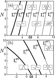
It follows from Fig. 1 that the branches are represented by monotonic (at least for moderate values of , and ) functions . Previous numerical results AlfZez2007 allow to conjecture that there are no solutions without linear counterpart for this potential. It is known that the solutions corresponding to the branches and in both, attractive and repulsive cases, are stable (see, e.g. for instance AlfZez2007 ; KevrekDyn and PelKevr2007 for more detailed analysis of perturbed solutions from ). Numerical calculations show that the modes from (the repulsive case) are unstable. In the attractive case the family corresponds to unstable modes for close to the bifurcation point . More specifically, in Ref. AlfZez2007 the instability has been observed for where . It has also been found that for the mode is stable.
III.2 Small-amplitude modes
Let us now analyze the stability of the branch , for both attractive and repulsive cases when lies close to the bifurcation point . In the bifurcation point (linear limit) the solutions of the eigenvalue problem (7) are the pairs , where
| (23a) | |||||
| (23b) | |||||
and is -th Hermite polynomial (see e.g. AS ).
The stability of small amplitude solutions can be studied using the formulas (18)-(22). Let us start with the case . The spectrum of the operator is equidistant and consists of the eigenvalues and the corresponding eigenfunctions are given by , . All the eigenvalues are simple and there is one zero eigenvalue. The eigenvalues of the operator are and they correspond to the same eigenfunctions , . This means that the spectrum of includes double eigenvalues , , one simple zero eigenvalue and infinitely many simple positive eigenvalues. The mechanism of emerging of double eigenvalues becomes transparent from Table 1. Each of the double eigenvalues has an invariant subspace spanned by two functions, and .
| 0-th | 1-st | 2-nd | 3-rd | 4-th | 5-th | |||
|---|---|---|---|---|---|---|---|---|
| Eigenf-n | … | |||||||
| 2 | 0 | -2 | -4 | -6 | -8 | |||
| 4 | 0 | 4 | 16 | 36 | 64 | |||
| 4 | 2 | 0 | -2 | -4 | -6 | |||
| 16 | 4 | 0 | 4 | 16 | 36 |
Following Ref. Kato we consider the matrices
If the eigenvalues of are and , , then for the double eigenvalue of splits into two simple eigenvalues of : where . Therefore, if the eigenvalues of any of the matrices , are complex, the instability of the small-amplitude solution takes place. It is important that since both, repulsive () and attractive () cases are described by the eigenvalues of the same matrices , the complex eigenvalues of for some means the instability of small-amplitude modes in both, repulsive and attractive cases.
Simple, but tedious algebra gives the expressions for the elements of the matrices :
Using Maple we calculated the eigenvalues of the matrix . The results are collected in Table 2 were we observe the following facts:
| C | C | |||||
|---|---|---|---|---|---|---|
| – | C | C | C | |||
| – | – | C | C | C | ||
| – | – | – | C | C | ||
| – | – | – | – | C | ||
| – | – | – | – | – |
(i) In columns 2 to 6 there is at least one letter “C” which means instability of small-amplitude modes belonging to the respective branch , for both, attractive and repulsive nonlinearities. We conjecture that the instability of small-amplitude modes takes place for all branches and with .
(ii) In the case the mode is stable. That confirms the results of KevrekDyn (see Fig. 1 there). It is interesting that in the limit the algebraic and geometric multiplicities of the eigenvalue are both equal to 2. At the same time two real eigenvalues emerging from the double eigenvalue for have opposite Krein signatures which do not correspond to the generic case (see MacKay1987 ).
(iii) When the matrix has a zero eigenvalue. This reflects the fact that
| (25) |
is an eigenfunction of the operator corresponding to for any mode belonging to any branch or .
III.3 Nonlinear modes of arbitrary amplitudes
In order to study the linear stability of the nonlinear modes of a finite amplitude we have first calculated the modes using a modified shooting method developed in Ref. AlfZez2007 and used in Refs. AlfZez2007 ; AZKV to compute different families of nonlinear modes. Then we have found numerically the eigenvalues of the operator . To do so we have approximated the solution on a grid, replacing the second derivatives in by second-order finite differences and calculated the eigenvalues of the resulting sparse matrix. The result is shown in Figs. 2 and 3. One can see that the families at possess two double eigenvalues (Fig. 2, panels b,c,e,f), (merged eigenvalues ) and , (merged eigenvalues ). These eigenvalues split; in the case of the resulting eigenvalues remain real and positive, one of them corresponding to the exact solution (25). In the case of , if the nonlinearity is attractive, there exist two complex eigenvalues on the interval , . At these eigenvalues merge and the mode becomes stable. Since the number of particles of the mode grows when moving along the branch , one can say that there is a threshold on number of particles for the stability of the mode in attractive case. If the nonlinearity is repulsive, the two complex eigenvalues do not disappear through all the region of parameter investigated; therefore the mode remains unstable. In the case of the family , (Fig. 3, (a)-(f)) at there are three double eigenvalues , and which split. Then the scenario is similar to the case of the family . The eigenvalues originated by remain real and one of them corresponds to the exact solution (25). In the attractive case the mode becomes stable after the two pairs of eigenvalues merge i.e. for ; at this point the second pair of the eigenvalues (both originated from ) merges. In the repulsive case the mode remains unstable through all the region of the parameter studied.
Summarizing, our results support that high-order modes of GPE with harmonic potential and attractive interactions, are stable when the number of particles exceeds a threshold value (different for each branch), what corroborates our analysis on the quasi-linear behavior of upper modes made in the begining of Sec. II.3. In the repulsive case, high-order modes of GPE with a harmonic potential are unstable. Our result contradicts those of Carr2001 where it was claimed that stable modes exist for both signs of nonlinear term.
IV Anharmonic potentials (I) : Small perturbations of a harmonic potential
Now we turn our attention to the GPE with a harmonic potential perturbed by a quartic term, , . In this case the eigenvalues and eigenfunctions , , for the linear problem (7) can be found numerically or by means of asymptotic procedures BendOrsz . Also one have to employ numerics for the construction of the branches of nonlinear modes and ; which are similar to the corresponding branches for harmonic potential case except for small deformations. As in the purely harmonic case, the branches are monotonic (at least for moderate values of , and ) and can be parametrized by any of the parameters and . However, the spectrum is no longer equidistant, which has several important consequences as we will discuss in what follows.
IV.1 Small amplitude modes
The stability of small amplitude modes belonging to the branches in the case of the anharmonic potential can be also studied by means of asymptotic expansions (18)-(22). Consider the case . The spectrum of the operator now consists of simple eigenvalues , , and the Krein signature of the eigenvalue is . Therefore, if is small the spectrum of contains pairs of close eigenvalues of opposite Krein signatures, and , , which are, nevertheless, different. The spectrum contains also a zero eigenvalue and an infinite sequence of increasing positive eigenvalues. Therefore, generally speaking, the spectrum , does not contain multiple eigenvalues.
When passing from to the eigenvalues of the operator vary continuously. Therefore, one can expect the stability of the mode until two eigenvalues with opposite Krein signature merge. So, the small amplitude modes are expected to be stable for all the branches and .
IV.2 Nonlinear modes of arbitrary amplitude: .
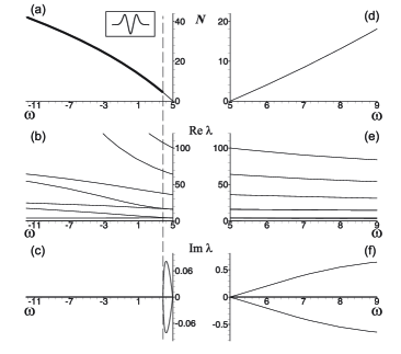
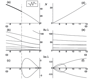
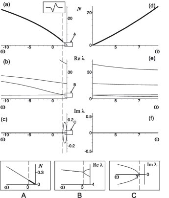
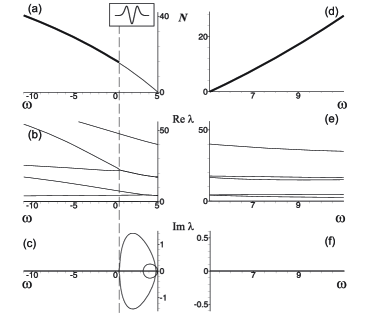
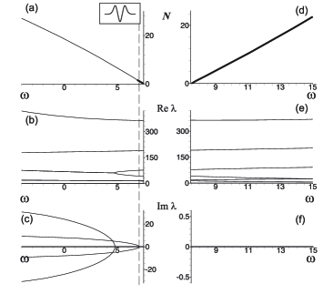
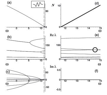
In order to study the linear stability of the nonlinear modes of a finite amplitude we have first calculated the spectrum of the operator numerically, concentrating on the branches for . The obtained general picture appears to be very different from that of the harmonic potential. The plots of real and imaginary parts of the eigenvalues vs for the branches , and in both attractive and repulsive cases are shown in Figs. 4, 5, and 6.
The general property of all the cases considered is that the instability of the nonlinear modes occurs only due to collisions of pairs of eigenvalues which are continuation of the respective eigenvalues and in the linear limit, i.e. of the eigenvalues of the operator . In what follows we call them -pairs. The eigenvalues in these pairs have opposite Krein signatures.
Then, the other numerical results can be structured as follows.
Repulsive nonlinearity.
The ground state modes corresponding to the branch are stable, since there are no -pair in the spectrum of . The modes from the next branch, , in the limit of strong nonlinearity correspond to “dark” soliton modes; there is one -pair in the spectrum of , but no collisions of eigenvalues have been found when tracing the modes of this branch within the range of parameter where it has been investigated (see Fig. 4, right panels). Therefore we conclude that the modes from are stable. A similar situation takes place for the branch where two -pairs in the spectrum of present: no collision has been observed within the range of parameter under consideration (see Fig. 5, right panels). However this is not the case for higher branches. For instance, the collisions of eigenvalues has been observed for nonlinear modes from . The spectrum of the operator includes three -pair and a collision of one of them (highest) at some large enough value of has been seen (see Fig. 5, right panels). After the point of collision (i.e. for greater values of ) the pair of collided eigenvalues become complex which means the instability of corresponding nonlinear modes. A similar situation takes place for the branch . In general, this points out to the fact that the instability of higher modes, generically, takes place, if the number of particles exceed some threshold value, which is particular for each branch . The existence of the threshold value for the branches and which we have not found in our numerical investigation needs more delicate analysis.
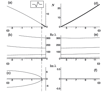
Attractive nonlinearity.
The ground state modes of the branch are stable. For the branch , there is one -pair in the spectrum of (see Fig. 4, left panels). Then there exist two bifurcation values of the parameter (the number of particles). When , increasing, reaches the first bifurcation value, the eigenvalues of this pair collide and become complex. For the values of below this threshold, the mode is stable; however, for the potential under consideration the first bifurcation value is very tiny, so it is not visible in Fig. 4. Then, when reaches the second bifurcation value, the complex eigenvalue collide again and become real. So, we can conclude that the modes of are stable unless the number of particles belongs to an instability window; the lower bound of this window is close to zero (but separated from zero). The size of the window of instability increases when grows and both bounds of this window are quite sensitive to variation of . A similar situation has been observed for higher branches of nonlinear modes. For instance, the spectrum of the operator spectrum of , the branch , includes two -pairs. As grows both of them undergo the same evolution: they become complex at first bifurcation value of and return to be real at the second bifurcation value (see Fig. 5, left panels). The interval with respect to between the first bifurcation value for the pair and second bifurcation value for the pair represents the window of instability. Upper boundary of this instability window is marked by dashed line in Fig. 5. However, since the first bifurcation value for the pair (lowest curve in Fig. 5, panel (b)) is very tiny, so the lower boundary of instability window cannot be separate from zero in Fig. 5. Therefore, the modes from are stable if does not belong to instability window. This situation, probably, is generic for other higher branches.
To confirm our results on the stability of nonlinear high-order modes we also have performed a series of direct numerical simulations of their evolution, perturbed by a random perturbation of 5% amplitude of the mode. Thus we have simulated the evolution of initial data of the form with a white noise of maximum amplitude 0.05. The subsequent dynamics of the modes under Eq. (5) was computed using a second order in time split-step pseudospectral scheme discretized in space using trigonometric polynomials (via the FFT). In all the cases studied, which included most of the branches presented here our test verified the predictions based on linear stability analysis.
IV.3 Nonlinear modes of arbitrary amplitude: .
Let us briefly summarize the stability results for the potential , and . In this case only a finite number of branches can exist, since there is a finite number of discrete eigenvalues for Eq.(7). These branches can be found numerically. The linear stability analysis performed for the potential shows (see Fig. 7) that all solutions of the branch which we have considered are linearly stable. On the other hand, the modes of are also stable, except some instability window situated close to the point of branching. This is in contrast with the case , since in that case the instability window is situated on the branch but not . The solutions of the branch are also linearly stable whereas the solutions of the branch are stable only in the vicinity of the branching point, i.e. only for . For the branches the picture of stability/instability becomes more complex.
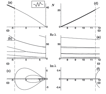
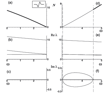
V Anharmonic potentials (II): Potential
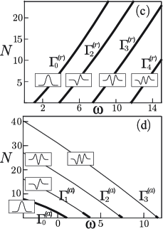
In order to show that the results for anharmonic potentials are quite generic, let us consider GPE with . Again, the eigenvalues, , and eigenfunctions , , for the linear problem (7) cannot be obtained exactly. The branches of nonlinear modes and which have been found numerically for are similar to the corresponding branches for harmonic potential case. These branches are monotonic (at least for moderate values of , and ) and can be parametrized by any of the parameters , .
Due to the reasons discussed above, the small amplitude solutions of GPE with the potential generically are stable for both, attractive and repulsive nonlinearities. In order to study the stability of nonlinear modes in general, we have analyzed the bifurcations of eigenvalues of when varies along the families and . Our numerical investigation shows that, as in the case of weak anharmonicity, the instability of nonlinear modes from occurs only due to collisions of those pairs of eigenvalues which are continuation of eigenvalues and in linear limit i.e. in the spectrum of . These eigenvalues and are of opposite Krein signature. Again, let us refer to these pairs of eigenvalues as -pairs.
Qualitatively, the stability picture for the case is the same as in the case , , except for some minor differences. The first one is that we have not found the threshold of instability in in the case of repulsive nonlinearity for the modes in the branches , . Therefore, these modes are stable in all the parameter range studied. Second, we have not found an upper bound of instability window in in the case of attractive nonlinearity for the modes from , . We believe that it is a technical problem related to the finiteness of the region studied but we think an upper bound of this instability window exists. The plots of real and imaginary parts of eigenvalues of the operator versus for the branches , and for attractive and repulsive nonlinearities are shown in Figs. 8, 9, and 10.
It is interesting to mention that we have also observed collisions of eigenvalues with opposite Krein signatures which belong to different -pairs. In our case they did not lead to instability since they remained real after the collision (see for example Fig. 10, panel (e)). This phenomenon does not correspond to a generic situation; it is caused by the opposite parity of colliding eigenfunctions (one of them was odd, while the other one was even).
We have also performed a set of direct numerical simulations of the evolution of perturbed stationary modes in Eq. (5) as described in Sec. IV.2. The outcome of those simulations confirms the results of the linear stability analysis.
| , | |||
| 0-th mode, (ground state), | stable | stable | stable |
| 1-st mode, small amplitude limit | stable | stable | stable |
| 1-st mode (”bright soliton”), general case | stable | unstable, if belongs to some “instability window”. The lower bound of this “window” is separated from zero. The size of the “window” grows with . Otherwise stable. | unstable, if belongs to some “instability window”, with lower bound separated from zero. Otherwise stable. |
| 1-st mode, small amplitude limit | stable | stable | stable |
| 1-st mode,(”dark soliton”) , general case | stable | stable for all which have been considered. | stable for all which have been considered. |
| Higher modes, small amplitude limit | unstable | stable | stable |
| Higher modes, , general case | stable, if exceeds a threshold. | unstable, if belongs to some “instability window”, with lower bound separated from zero. The size of the “window” grows with . Otherwise stable. | Hypothetically, unstable, if lies in a large “window” of instability. The upper boundary of this “window” has not been found in our numerics. |
| Higher modes, small amplitude limit | unstable | stable | stable |
| Higher modes, , general case | unstable | Hypothetically unstable, if exceeds some threshold. Otherwise stable. | stable for all which we have considered. |
VI Conclusions and discussion
Using a combination of different analytical and numerical tools including the analysis of the small amplitude limit, the nonlinear WKB approximation, the Krein signature and direct numerical simulations we have analyzed the stability properties of higher-order nonlinear trapped modes for the GPE with different potentials. First, we have reviewed the results for the harmonic potential and discussed how the stability of the modes is essentially affected by the fact that levels are equidistant. Next, we have considered the weakly anharmonic potential , . Our results, summarized in Table 3, lead to the conclusion that even a small anharmonicity which does not affect essentially the shape of the modes, improves drastically the stability properties of higher-order modes due to the fact that none of these potentials has an equidistant spectrum. We conjecture that the same situation would take place also for more generic perturbation of harmonic potential, for instance, by non-symmetric (e.g. cubic) perturbation.
Then we have checked that in the case of stronger anharmonicity the stability/instability picture is similar to the case of potential , , . We have studied the GPE with the potential (the details have not been discussed in this paper) and found that they reproduce the same essential features.
It follows form the arguments presented, that the scenario for appearance of instability induced by the equidistant spectrum of the harmonic oscillator holds also for other classes of potentials with equidistant spectra (for construction of such potentials see Equidistant1 ; Equidistant2 ; Equidistant3 ) or, more generally, for potentials for which the spacing between some levels (not necessarily adjacent) are equal. In that situation, the splitting of double eigenvalues for the operator can lead to complex eigenvalues in the linear stability problem.
An interesting point for further investigation, is the effect of the type of confining potential on the stability of higher order modes in two spatial dimensions, e.g. the stability of vortices under deformations of the potential. This subject has attracted a lot of attention in the last years VP1 ; VP2 ; VP3 ; VP4 ; Fin1 ; Michalache2006 ; Fin2 ; RadSymmKevrek2007 ; Watanabe and the methodology developed in this paper could be useful. In fact, the situation is similar to the one considered above. In the case of harmonic potentials the spectrum of corresponding eigenvalue problem is equidistant; the corresponding eigenfunctions are Gauss-Laguerre modes. Then, one can expect that switching to anharmonic potentials can also change the stability properties of vortices and other higher order modes.
Finally, we would like to mention another practical implication of the enhanced stability of nonlinear modes by the anharmonicity of the trap potential. As it was suggested in KevrekDyn such modes can grow from the eigenstates of the linear oscillator by increasing the nonlinearity using Feshbach resonance management (in the language of this paper this corresponds to the “motion” along a nonlinear branch starting from the bifurcation point as the number of particles increases starting from zero). This fact can be used for the generation of single solitons or even solitonic trains. The instability of the nonlinear modes in the case of the harmonic potential was the major obstacle for the practical implementation of that mechanism. However, the idea becomes experimentally feasible if an anharmoic potential is used since now higher order branches have a different stability and thus can lead to stable solitons.
Acknowledgements.
GA acknowledges the support from the President Program for Leading Scientific Schools (Project 3826.2008.2.). The work of VVK was supported by the grant POCI/FIS/56237/2004 (European Program FEDER and FCT, Portugal). VMPG is partially supported by grants FIS2006-04190 (Ministerio de Educación y Ciencia, Spain) and PCI-08-0093 (Junta de Comunidades de Castilla-La Mancha, Spain).References
- (1) C. J. Pethick and H. Smith Bose-Einstein Condensation in Dilute Gases (Cambridge University Press,Cambridge, England, 2001); L. P. Pitaevskii, S. Stringari, Bose-Einstein condensation, Oxford (2003); Emergent Nonlinear Phenomena in Bose-Einstein Condensates Theory and Experiment Eds. P. G. Kevrekidis, D. J. Frantzeskakis, and R. Carretero-González (Springer, 2008).
- (2) M. H. Anderson, J. R. Ensher, M. R. Matthews, C. E. Wieman and E. A. Cornell, Science, 269, 198 (1995).
- (3) C. C. Bradley, C. A.Sackett, J. J. Tollett and R. G. Hulet, Phys. Rev. Lett. 75, 1687 (1995)
- (4) M. Edwards and K. Burnett, Phys. Rev. A, 51, 1382 (1995); F. Dalfovo and S. Stringari, Phys. Rev. A, 53, 2477 (1996); P. A. Ruprecht, M. J. Holland, K. Burnett and M. Edwards, Phys. Rev. A, 51, 4704 (1995).
- (5) V. I. Yukalov, E. P. Yukalova, and V. S. Bagnato, Phys. Rev. A 56, 4845 (1997); V. I. Yukalov, E. P. Yukalova and V. S. Bagnato, Phys. Rev. A, 66 043602 (2002); M. Brtka, A. Gammal and L. Tomio, Phys. Lett. A, 359, 339 (2006).
- (6) Yu. S. Kivshar, T. J. Alexander and S. K.Turitsyn, Phys. Lett. A, 278, 225 (2001).
- (7) R. D’Agosta, B. A. Malomed and C. Presilla, Laser Physics, 12, 37 (2002).
- (8) R. D’Agosta and C. Presilla, Phys. Rev. A, 65, 043609 (2002).
- (9) V. V. Konotop and P. G. Kevrekidis, Phys. Rev. Lett. 91, 230402 (2003).
- (10) P. G. Kevrekidis, V. V. Konotop, A. Rodrigues, and D. J. Frantzeskakis, J. Phys. B: At. Mol. Opt. Phys. 38, 1173 (2005).
- (11) G. Alfimov and D. Zezyulin, Nonlinearity, 20, 2075 (2007).
- (12) D. E. Pelinovsky and P. G. Kevrekidis, arXiv.org/abs/cond-mat/0705.1016
- (13) L. D. Carr, J. N. Kutz and W. P. Reinhardt, Phys.Rev. E, 63, 066604 (2001).
- (14) V. M. Pérez-García, H. Michinel, H. Herrero, Phys. Rev. A 57, 3837 (1998).
- (15) J. J. García-Ripoll, G. Molina-Terriza, V. M. Pérez-García, and L. Torner, Phys. Rev. Lett. 87, 140403 (2001).
- (16) L.-C. Crasovan, G. Molina-Terriza, J. P. Torres, L. Torner, V. M. Pérez-García, D. Mihalache, Phys. Rev. E 66, 036612 (2002).
- (17) L.-C. Crasovan, V. Vekslerchik, V. M. Pérez-García, J. P. Torres, D. Mihalache, and L. Torner, Phys. Rev. A 68, 063609 (2003).
- (18) L.-C. Crasovan, V. M. Perez-Garcia, I. Danaila, D. Mihalache, Ll. Torner, Phys. Rev. A 70, 033605 (2004).
- (19) M. Mottonen, S. M. M. Virtanen, T. Isoshima, and M. M. Salomaa, Phys. Rev. A 71, 033626 (2005).
- (20) D. Michalache, D. Mazilu, B. A. Malomed, F. Lederer, Phys.Rev.A, 73, 043615 (2006).
- (21) V. Pietila, M. Mottonen, T. Isoshima, J. A. M. Huhtamaki and S. M. M. Virtanen, Phys Rev. A 74, 023603 (2006).
- (22) G. Watanabe, and C. J. Petick, cond-mat/0701270
- (23) G.Herring, L. D. Carr, R. Carretero-González, P. G. Kevrekidis and D. J. Frantzeskakis. Phys. Rev. A, 77, 023625 (2008)
- (24) D. A. Zezyulin, G. L. Alfimov, V. V. Konotop, V. M. Pérez-García, Phys. Rev. A 76, 013621 (2007).
- (25) R. S. MacKay, Stability of equilibria of Hamiltonian systems, in Hamiltonian Dynamical Systems, R.S.MacKay and J.Meiss eds, Adam Hilger, 1987, pp. 137-153.
- (26) I. M. Gelfand. Lectures on Linear Algebra, Dover Publications (1989).
- (27) T. Kato, Perturbation theory for linear operators, Springer-Verlag, Berlin - Heidelberg -Ney-York (1966).
- (28) C. M. Bender, S. A. Orszag. Advanced mathematical methods for scientists and Engeneers, McGraw-Hill book company, 1978.
- (29) M. Kunze, T. Kupper, V. K. Mezentsev, E.G.Shapiro and S.K Turitsyn, Physica D, 128, 273 (1999)
- (30) Handbook of Mathematical Functions, M. Abramovitz and I. A. Stegun, eds, (National Bureau of Standards, 1972)
- (31) G. Szegö, Orthogonal polynomials, Amer.Math.Soc, Colloquium publ, V. XXIII, Providence, Rhode Island (1939).
- (32) V. M. Eleonsky and V. G. Korolev, J. Phys. A: Math. Gen., 28, 4973 (1995)
- (33) V. M. Eleonsky and V. G. Korolev, Phys. Rev. A, 55, 2580, (1997)
- (34) J. Morales, J. J. Peña, A. Rubio-Ponce, Theor. Chem. Accounts, 110, 403 (2003).