Optimization of operational aircraft parameters Reducing Noise Emission

Abstract.

The objective of this paper is to develop a model and a minimization method to provide flight path optimums reducing aircraft noise in the vicinity of airports. Optimization algorithm has solved a complex optimal control problem, and generates flight paths minimizing aircraft noise levels. Operational and safety constraints have been considered and their limits satisfied. Results are here presented and discussed.

Nomenclature

$$\begin{array}[]{llllll}\hline\cr\\ C_{z_{\alpha}}&&\textrm{slope of lift coefficient curve}&\delta_{x}&&\textrm{throttle setting}\\ C_{x_{0}}&&\textrm{drag coefficient}&k_{i}&&\textrm{induced drag parameter}\\ T&&\textrm{thrust},N&V&&\textrm{speed of aircraft},m/s\\ L&&\textrm{lift, N}&S&&\textrm{wing area},m^{2}\\ D&&\textrm{drag, N}&c&&\textrm{speed of sound},m/s\\ g&&9.8\,m/s^{2}&M&&\textrm{mach number},V/c\\ x&&\textrm{horizontal distance},m&\rho&&\textrm{air density},kg/m^{3}\\ y&&\textrm{lateral distance},m&d&&\textrm{nozzle diameter},m\\ h&&\textrm{aircraft height},m&s&&\textrm{area of coaxial engine nozzle},m^{2}\\ k&&\textrm{induced drag coefficient}&v&&\textrm{speed of gas},m/s\\ t&&\textrm{time},s&w&&\textrm{density exponent}\\ \mu&&\textrm{roll angle},rad&\tau&&\textrm{temperature, K}\\ \alpha&&\textrm{angle of attack},rad&\theta&&\textrm{directivity angle},rad\\ \gamma&&\textrm{flight path angle},rad&R&&\textrm{source-to-observer distance},m\\ \chi&&\textrm{yaw angle},rad&m&&\textrm{aircraft mass},kg\\ \\ \hline\cr\\ \\ \end{array}$$

1. Introduction

Since the introduction of jet aircraft in the 1960, aircraft noise produced in the vicinity of airports has represented a serious social and environmental issue. It is a continuing source of annoyance in nearby communities. The importance of that problem has been highlighted by the increased public concern for environmental
issues. To deal with this problem, aircraft manufacturers and public establishments are engaged in research on technical and theoretical approaches for noise reduction concepts that should be applied to new aircraft. The ability to assess noise exposure accurately is an increasingly important factor in the design and implementation of any airport improvements.

Aircraft are complex noise sources and the emitted intensities vary with the type of aircraft, in particular, with the type of engines and with the implemented flight procedures. The noise contour assessment due to the variety of flight route schemes and predicted procedures is also complex. A set of data must be used which includes noise data, flight path parameters and their features, and environmental conditions affecting outdoor sound propagation. Three development initiatives are available for the reduction of aircraft noise: (1) innovative passive technologies required by the industry for developing environmentally compatible and economically viable aircraft, (2) advanced active technologies such as computational aeroacoustics, active control, advanced propagation and prediction methods, (3) reliable trajectory and procedures optimization which can be used to determine optimal landing approach for any arbitrary aircraft at any given airport. The last action will be particularly emphasized in the next sections.

A number of calculation programs of aircraft noise impact have been developed over the last 30 years. They have been widely used by aircraft manufacturers and airport authorities. Their reliability and results efficiency to assess the real impact of aircraft noise have not been proved conclusively. They are complex, very slow and can not be planned for on-line and on-site use. That is the reason why, the model described in this paper, generating optimal trajectories minimizing noise, is considered as a promising scientific plan.

Several optimization codes for NLP exist in the literature. After a large number of test and comparisons, we choose KNITRO [7] which known for its performances and robustness, this software is efficient to solve general nonlinear programming. We will explain in the following sections how the considered optimal control problem is discretized and solved. Numerical results have been analyzed and their reliability and flexibility have been proved. We have demonstrated the effectiveness of computation and its application to aircraft noise reduction. The objective of that alternative research is to develop high payoff models to enable a safe, and environmentally compatible and economical aircraft. We should make large profits in terms of noise abatement in comparison with the expected noise control systems in progress. These systems, which are not in an advanced step, in particular at low frequencies, are still ineffective or impractical. Actually, the low-frequency broadband generated by the engines represents a significant source of environmental noise. Their radiation during flight operations is extremely difficult to attenuate using the mentioned systems and is capable of propagating over long distance [21].

Details of trajectory and aircraft noise models, and optimal control problems are presented in section 2 and 3 while the last section is devoted to numerical experiments.

2. Optimal Control Problem

2.1. Equation of Motion

In general, the system of differential equations commonly employed in aircraft trajectory analysis is the following six-dimension system derived at the center of mass of aircraft :

$$(ED)\quad\quad\left\{\begin{array}[]{lll}\dot{V}&=&g\left(\displaystyle\frac{T\cos\alpha-D}{mg}-\sin\gamma\right)\\ \\ \dot{\gamma}&=&\displaystyle\frac{1}{mV}\left((T\sin\alpha+L)\cos\mu-mg\cos\gamma\right)\\ \\ \dot{\chi}&=&\displaystyle\frac{(T\sin\alpha+L)\sin\mu}{mV\cos\gamma}\\ \\ \dot{x}&=&V\cos\gamma\cos\chi\\ \\ \dot{y}&=&V\cos\gamma\sin\chi\\ \\ \dot{h}&=&V\sin\gamma\\ \end{array}\right.$$

where $T=T(h,V,\delta_{x}),D=D(h,V,\alpha)$ and $L=L(h,V,\alpha)$.
These equations embody the assumptions of a constant weight, symmetric flight and constant gravitational attraction [1, 6].

Figure ($1$) shows the forces acting on an aircraft at its center of gravity during an approach.

Figure 1. Aircraft forces during phase of descent

Those equations could be applied to conventional aircraft of all sizes. The most dominant aerodynamics affecting results are the lift $L$ and drag $D$, defined as follows [6]

$$\begin{array}[]{ll}L=\frac{1}{2}\rho SV^{2}C_{z_{\alpha}}\alpha\\ \\ D=\frac{1}{2}\rho SV^{2}\left[C_{x_{0}}+k_{i}C_{z_{\alpha}}^{2}\alpha^{2}\right]\\ \end{array}$$

The thrust model chosen, by Matthingly [13], depends explicitly on the aircraft speed, the geometric aircraft height and the throttle setting

$$T=T_{0}\delta_{x}\displaystyle\frac{\rho}{\rho_{0}}\left(1-M+\displaystyle\frac{M^{2}}{2}\right)$$

$T_{0}$ is full thrust, $\rho_{0}$ is atmospheric density at the ground $(=1.225\,\,kg/m^{3})$ and $\rho$ is atmospheric density at the height $h\,(\rho=\rho_{0}(1-22.6\times 10^{-6}h)^{4.26})$.

The previous system of equations  (2.1)  can be written in the following generic
form :

$$\begin{array}[]{l}\\ \dot{X}(t)=f(X(t),U(t))\\ \end{array}$$

where :

$$\begin{array}[]{cccl}X:&[t_{0},t_{f}]&\longrightarrow&I\!\!R^{6}\\ &t&\longrightarrow&X(t)=[V(t),\gamma(t),\chi(t),x(t),y(t),h(t)]\;\textrm{are the state variables,}\\ \\ U:&[t_{0},t_{f}]&\longrightarrow&I\!\!R^{3}\\ &t&\longrightarrow&U(t)=[\alpha(t),\delta_{x}(t),\mu(t)]\;\textrm{are the control variables,}\\ \end{array}$$

and $t_{0}$ and $t_{f}$ are the initial and final times.

2.2. Constraints

Search for optimal trajectories minimizing noise must be done in a realistic flight domain. Indeed, operational procedures are performed with respect to parameter limits related to the safety of flight and the operational modes of the aircraft.

• The throttle stays in some interval

  $$\delta_{x_{min}}\leq\delta_{x}\leq\delta_{x_{max}}$$

• The speed is bounded

  $$1.3V_{s_{0}}\leq V\leq V_{max}$$

  where $V_{s_{0}}$ the stall velocity, the limited velocity at which the aircraft can produce enough lift to balance the aircraft weight. $V_{s_{0}}$ and $V_{max}$ depend on the type of aircraft.
  

• The flight path angle providing a measure of the angle of the velocity to the inertial horizontal axis, is bounded

  $$\gamma_{min}\leq\gamma\leq\gamma_{max}$$

• The angle of attack is bounded

  $$\alpha_{min}\leq\alpha\leq\alpha_{max}$$

• The yaw angle and roll angle stay in some prescribed interval

  $$\begin{array}[]{lll}\chi_{min}&\leq\chi&\leq\chi_{max}\\ \mu_{min}&\leq\mu&\leq\mu_{max}\\ \end{array}$$

Those inequality constraints could be formulated as:

$$\begin{array}[]{l}a\leq C(X(t),U(t))\leq b\end{array}$$

where

(1) $$\begin{array}[]{llll}C:&I\!\!R^{6}\times I\!\!R^{3}&\longrightarrow&I\!\!R^{6}\\ &(X(t),U(t))&\longrightarrow&C(X(t),U(t))=[\gamma(t),V(t),\chi(t),\alpha(t),\delta_{x}(t),\mu(t)]\end{array}$$

$a$ and $b$ are two constant vectors of $I\!\!R^{6}$.

2.3. Cost function

Models and methods used to assess environmental noise problems must be based on the noise exposure indices used by relevant international noise control regulations and standards (ICAO [9, 10], Lambert and Vallet [9]). As described by Zaporozhest and Tokarev [29], these indices vary greatly one from another both in their structure, and in the basic approaches used in their definitions.

The cost function to be minimized may be chosen as any usual aircraft noise index, which describes the effective noise level of the aircraft noise event [29, 30], like $SEL$ (Sound Exposure Level), the $EPNL$ (Effective Perceived Noise Levels) or the $L_{eq,\Delta t}$ (Equivalent noise level), … It is well known that the magnitude of $L_{eq,\Delta t}$ correlates well with the effects of noise on human activity, in particular, with the percentage of highly noise-annoyed people living in regions of significant aircraft noise impact. This criterion is commonly used, as basis, for the regulatory basis in many countries. Based on comparison of noise exposure indices and a comparison of the methodologies used to calculate the aircraft noise exposure, it can be concluded that the general form of the most used and accepted noise exposure index is $L_{eq,\Delta t}$ that we have chosen as an index ([11, 15]). $L_{eq,\Delta T}$ is expressed by:

(2) $$\begin{array}[]{ll}L_{eq,\Delta T}&=10\log\displaystyle\frac{1}{\Delta T}\int_{t_{0}}^{t_{f}}10^{0.1L_{P}(t)}dt\end{array}$$

where $t_{0}$ initial time, $t_{f}$ final time, $\Delta T=t_{f}-t_{0}$ and $L_{P}(t)$ is the overall sound pressure level (in decibels).

We will define in the next subsection the analytic method to compute the noise level at any reception point.

Calculation method for aircraft noise levels

The aircraft noise levels $L_{P}$ at a receiver is obtained by the following formula based on works [16, 31]:

(3) $$L_{P}=L_{ref}-20\log_{10}R+\Delta_{atm}+\Delta_{ground}+\Delta_{V}+\Delta_{D}+\Delta_{f}$$

where $L_{ref}$ is the sound level at the source, $20\log_{10}R$ is a correction due to geometric divergence, $\Delta_{atm}$ is the attenuation due to atmospheric absorption of sound. The other terms $\Delta_{ground},\Delta_{V},\Delta_{D},\Delta_{f}$ correspond respectively to the ground effects, correction for the Doppler, correction for duration emission and correction for the frequency.

In this paper, we have used a semi-empirical model to predict noise generated by conventional-velocity-profile jets exhausting from coaxial nozzles predicting the aircraft noise levels represented by the jet noise [22] which corresponds to the main predominated noisy source. It is known that jet noise consists of three principal components. They are the turbulent mixing noise, the broadband shock associated noise and the screech tones. At the present time, this first approximation have been used herein. It seems to be correct in that step of research because the complexity of the problem. Many studies have agreed with this model and full-scale experimental data even at high jet velocities in the region near the jet axis. Numerical simulation of jet noise generation is not straightforward undertaking. Norum and Brown [17], Tam and Auriault [23, 24, 25] had earlier discussed some of the major computational difficulties anticipated in such effort. At the present time, there are reliable to jet noise prediction. However, there is no known way to predict tone intensity and directivity; even if it is entirely empirical. This is not surprising for the tone intensity which is determined by the nonlinearities of the feedback loop. Obviously, to complete this study we will need to integrate other noise source models in particular aerodynamics.

Although the numerous aspects of the mechanisms of noise generation by coaxial jets are not fully understood, the necessity to predict jet noise has led to the development of empirical procedures and methods. During the descent phase, the jet aircraft noise as well as propeller aircraft noise is approximately omni-directional and the noise emission is decreasing with decreasing speed when assuming that the power setting is constant. The jet noise results from the turbulence created by the jet mixing with the surrounding air. Jet mixing noise caused by subsonic jets is broadband in nature (its frequency range is without having specific tone component) and is centered at low frequencies. Subsonic jets have additional shock structure-related noise components that generally occur at a higher frequencies. The prediction of jet noise is extremely complex. The used methods in system analysis and in the engine design usually employed simpler or semi-empirical prediction techniques. By replacing the predicted jet noise level [22] in (3), we obtain the following expression

(4) $$L_{P}(t)=\left\{\begin{array}[]{ll}&141+10\log_{10}\left(\displaystyle\frac{\rho_{1}}{\rho}\right)^{w}+10\log_{10}\left(\displaystyle\frac{V_{e}}{c}\right)^{7.5}+3\log_{10}\left(\displaystyle\frac{2s_{1}}{\pi d^{2}}+0.5\right)\\ \\ &+10\log_{10}\left(\left(1-\displaystyle\frac{v_{2}}{v_{1}}\right)^{me}+1.2\displaystyle\frac{\left(1+\displaystyle\frac{s_{2}v_{2}^{2}}{s_{1}v_{1}^{2}}\right)^{4}}{\left(1+\displaystyle\frac{s_{2}}{s_{1}}\right)^{3}}\right)+10\log_{10}s_{1}\\ \\ &+\log_{10}\displaystyle\frac{\tau_{1}}{\tau_{2}}+10\log_{10}\left(\left(\displaystyle\frac{\rho}{\rho_{ISA}}\right)^{2}\left(\displaystyle\frac{c}{c_{ISA}}\right)^{4}\right)\\ \\ &-20\log_{10}R-15\log_{10}(C_{D}(M_{c},\theta))-10\log_{10}(1-M\cos\theta),\end{array}\right.$$

where

$$\begin{array}[]{rll}v_{1}&&\textrm{speed of jet gas at inner contours}\\ v_{2}&&\textrm{speed of jet gas at outer contours}\\ s_{1}&&\textrm{area of coaxial engine nozzle at inner contours}\\ s_{2}&&\textrm{area of coaxial engine nozzle at outer contours}\\ \tau_{1}&&\textrm{temperature at inner contours}\\ \tau_{2}&&\textrm{temperature at outer contours}\\ \rho_{1}&&\textrm{atmospheric density at inner contours}\\ \rho_{ISA}&&\textrm{International Standard Atmosphere density}\\ c_{ISA}&&\textrm{International Standard Atmosphere for speed of sound.}\\ \end{array}$$

The effective speed $V_{e}$ is defined by:

$$V_{e}=v_{1}[1-(V/v_{1})\cos(\alpha_{T})]^{2/3}.$$

The angle of attack $\alpha_{T}$, the upstream axis of the jet relative to the direction of aircraft motion has been neglected in this study.
The distance source to the observer is

$$\begin{array}[]{l}R=(x-x_{obs})^{2}+(y-y_{obs})^{2}+h^{2}\end{array}$$

where $(x_{obs},y_{obs})$ are the coordinates of the observer. $\Delta_{V}$ is expressed by

$$\begin{array}[]{l}\Delta_{V}=-15\log(C_{D}(M_{c},\theta))-10\log(1-M\cos\theta)\end{array}$$

where $C_{D}(M_{c},\theta)$ indicate the Doppler convection factor:

$$C_{D}(M_{c},\theta)=[(1+M_{c}\cos\theta)^{2}+0.04M_{c}^{2}],$$

the Mach number of convection is:

$$M_{c}=0.62(v_{1}-V)/c$$

and $w=\displaystyle\frac{3({V_{e}/c})^{3.5}}{0.6+(V_{e}/c)^{3.5}}-1$.

The validity of this improved prediction model is established by fairly extensive comparisons with model-scale static data [26]. Insufficient appropriate simulated-flight data are available in the open literature, so verification of flight effects during aircraft descent has to be established. Analysis by Stone and al. [22] has shown that measured data are used to calibrate the behavior of the used jet noise model and its implications from theory. Nowadays, the above formulation is being considered realistic compared to others described in applied and fundamental literature dealing with jet noise of aircraft during descent operations.

Taking account the formulas (2) and (4), we obtain our cost function in the following integral function form

$$\begin{array}[]{cll}J:\mathcal{C}^{1}([t_{0},t_{f}],I\!\!R^{6})\times\mathcal{C}^{1}([t_{0},t_{f}],I\!\!R^{3})&\longrightarrow&I\!\!R\\ (X(t),U(t))&\longrightarrow&J(X(t),U(t))=\displaystyle\int_{t_{0}}^{t_{f}}\ell(X(t),U(t))dt\end{array}$$

$J$ is the criterion for optimizing the noise level at the reception point. It doesn’t depend of $\chi,\;\gamma$ and $U$.

2.4. Optimal Control Problem

Finding an optimal trajectory, in term of minimizing noise emission during a descent, can be mathematically stated as an ODE optimal control problem. We opted different notations $z\equiv X,u\equiv U$ and $t_{0}=0$:

($$OCP \left\{\begin{array}[]{l}min\ J(z,u)=\displaystyle\int_{0}^{t_{f}}\ell(z(t),u(t))dt\\ \\ \dot{z}(t)=f(z(t),u(t)),\forall t\,\in[0,t_{f}]\\ \\ z_{I_{1}}(0)=c_{1},\,z_{I_{2}}(t_{f})=c_{2}\\ \\ a\leq C(z(t),u(t))\leq b\end{array}\right.$$)

where $J:I\!\!R^{n+m}\rightarrow I\!\!R,f:I\!\!R^{n+m}\rightarrow I\!\!R^{n}$ and $C:I\!\!R^{n+m}\rightarrow I\!\!R^{q}$ correspond respectively to the cost function, the dynamic of the problem, and the constraints defined in the previous section. The initial and final values for the sate variables $((x(0),y(0),h(0),V(0))$ and $(x(t_{f}),y(t_{f}),h(t_{f}))$ are fixed. $n_{\ell}:=|I_{1}|+|I_{2}|$ is the total number of fixed limit values of the state variables.

To solve our problem (find the optimal control $u(t)$ and the corresponding optimal state $z(t)$), we discretize the control and the state with identical grid and transcribe optimal control problem into nonlinear problem with constraints. The next section may be helpful in telling how the problem could be solved. They will present theoretical consideration and computational process that yield to flight paths minimizing noise levels at a given receiver.

3. Discrete Optimal Control Problem

To solve $(OCP)$ different methods and approaches can be used [3, 28]. In this paper, we use a direct optimal control technique : we first discretize $(OCP)$ and then solve the resulting nonlinear programming problem.

3.1. Discretization

We use an equidistant discretization of the time interval as

$$0=t_{0}<...<t_{N}=t_{f}$$

where :

$$t_{k}=t_{0}+k{\rm h},\;\;k=0,...,N\;\;\textrm{and}\;\;{\rm h}=\displaystyle\frac{t_{f}-t_{0}}{N}.$$

Then we consider that $u(.)$ is parameterized as a piecewise constant function :

$$u(t):=u_{k}\;\;\textrm{for}\;\;t\in[t_{k-1},t_{k}[$$

and use a Runge-Kutta scheme (Heun) to discretize the dynamic :

$$\left\{\begin{array}[]{l}z_{k+1}=z_{k}+{\rm h}\displaystyle\sum_{i=1}^{s}b_{i}f(z_{ki},u_{k})\\ z_{ki}=z_{k}+{\rm h}\displaystyle\sum_{j=1}^{s}a_{ij}f(z_{kj},u_{k})\\ k=0,\ldots,N-1,\quad i=1,\ldots,s.\\ \end{array}\right.$$

The new discrete objective function is stated as :

$$\tilde{J}=\displaystyle\sum_{k=0}^{N}\ell(z_{k},u_{k}).$$

The continuous optimal control problem $(OCP)$ is replaced by the following discretized control problem :

$$(NLP)\quad\quad\left\{\begin{array}[]{l}\min\displaystyle\sum_{k=0}^{N}\ell(z_{k},u_{k})\\ z_{k+1}=z_{k}+{\rm h}\displaystyle\sum_{i=1}^{s}b_{i}f(z_{ki},u_{k}),\quad k=0,\ldots,N-1\\ z_{ki}=z_{k}+{\rm h}\displaystyle\sum_{j=1}^{s}a_{ij}f(z_{kj},u_{k}),\quad k=0,\ldots,N-1\\ z_{0_{I_{1}}}=c_{1},\;\;z_{N_{I_{2}}}=c_{2}\\ \\ a\leq C(z_{k},u_{k})\leq b,\quad k=0,\ldots,N\\ \end{array}\right.$$

To solve (NLP) we developped an AMPL [2] model and used a robust interior point algorithm KNITRO [7]. We choose this NLP solver after numerous comparisons with some other standard solvers available on the NEOS (Server for Optimization) platform.

4. Numerical results

For different cases and configurations, we consider an aircraft approach with an initial condition $(x_{0}=0;y_{0}=0;h_{0}=3500\,m)$ a final condition $(x_{f}=60000\;m;y_{f}=5000\;m;h_{f}=500\;m)$ and for a fixed $tf=10$ min and a discretization parameter $N=100$ or $N=200$.
We first consider the simplest configuration of one single observer and no additional constraint.

4.1. One fixed observer

For various positions $(x_{obs},y_{obs})$ of an observer on the ground (near the aircraft trajectory) we calculate the optimal noise level $J$ (corresponding to our optimal trajectory $Tr$) and the noise level $J_{1}$ corresponding to the trajectory $Tr_{1}$ that minimizes the "fuel consumption" (re minimizing) the simple following model of consumption [6]:

$$CO(h,V,\delta_{x})=\int_{0}^{t_{f}}C_{SR}T(t)dt$$

where $C_{SR}$ is supposed constant.


The following table summarizes the obtained results.

$$\begin{array}[]{|c|c|c|c|c|c|c|}\hline\cr(x_{obs},y_{obs})&J\,(dB)&max(f.e,o.e)&\textrm{CPU}\,(s)&J_{1}(dB)&J_{1}-J(dB)&\%CO\\ \hline\cr\hline\cr(0,0)&45.92&7.92e-07&10&47.03&1.1&36\%\\ \hline\cr(0,2500)&44.95&8.76e-07&8.4&46.32&1.4&36\%\\ \hline\cr(0,5000)&43.27&3.44e-07&9.8&44.93&1.7&36\%\\ \hline\cr\hline\cr(20000,0)&48.97&4.66e-07&10.4&51.04&2.10&33\%\\ \hline\cr(20000,2500)&49.58&2.81e-08&10.6&51.55&2&26\%\\ \hline\cr(20000,5000)&47.18&8.36e-07&9.8&49.70&2.5&36\%\\ \hline\cr\hline\cr(40000,0)&47.59&6.73e-07&14.6&49.52&2&26\%\\ \hline\cr(40000,2500)&50.76&4.21e-07&6.9&52.87&2.11&26\%\\ \hline\cr(40000,5000)&49.74&6.92e-07&11.9&51.72&2&24\%\\ \hline\cr\hline\cr(60000,0)&42.85&5.29e-07&7.2&45.00&2.15&34\%\\ \hline\cr(60000,2500)&45.04&6.90e-07&6.7&48.014&3&36\%\\ \hline\cr(60000,5000)&48.84&7.10e-07&6&54.18&5.34&38\%\\ \hline\cr\end{array}$$

Table 1. Noise minimization

For each case, the algorithm (KNITRO[7]) found a solution with a very high accuracy. The computation of $Tr_{1}$ have been done only one time; it needs $7s$ with an accuracy of $max(f.e,o.e)=4.24e-07$.

The third column of Table $1$ measure the maximum of feasibility error and optimality error, the fourth one gives an idea on the computation effort (namely the CPU time). The two last columns correspond to the noise reduction and $\%$ of exceeded consumption : $\%CO=(CO(Tr)-CO(Tr_{1}))/CO(Tr)$.
Our trajectory that minimizes the noise consume about $31\%$ more than the trajectory minimizing the consumption.


The following figure showing the solution trajectory $Tr$, where the fixed observer presents a certain area near the airport :

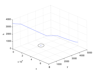
Figure 2. Trajectory in 3D

The following figures present the state and control variables of the optimal trajectory $Tr$.

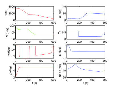
Figure 3. Solutions of $(NLP)$

We remark that the optimal variables $h,V,\chi,\alpha$ and $\mu$ present some large constant stages, while $\gamma$ and $\delta_{x}$ are bang-bang.

4.1.1. One fixed observer with an additional consumption constraint

Table (1) shows that the optimal trajectory $Tr$ consumes about $31\%$ more that $Tr_{1}$. This fact makes of interest some additional constraint on the consumption.

We define a new problem :

(5) $$(OCP)_{2}\quad\left\{\begin{array}[]{l}\min\,L_{eq,\Delta t}\\ \dot{z}(t)=f(z(t),u(t))\\ z_{I_{1}}(0)=c_{1},\,z_{I_{2}}(t_{f})=c_{2}\\ CO(z(t),u(t))<=1.1CO(Tr_{1})\\ \end{array}\right.$$

This problem can be solved using the same techniques (discretization,…) and the same configurations. We obtain the following results.

$$\begin{array}[]{|c|c|c|c|c|c|c|c|c|}\hline\cr(x_{obs},y_{obs})&J\,(dB)&max(f.e,o.e)&J_{1}(dB)&\textrm{CPU}\,(s)\\ \hline\cr\hline\cr(0,0)&46.32&9.94e-07&47.03&9.6\\ \hline\cr(0,2500)&45.44&9.17e-07&46.32&13.2\\ \hline\cr(0,5000)&43.94&9.49e-07&44.93&13.1\\ \hline\cr\hline\cr(20000,0)&49.79&7.25e-07&51.04&18.6\\ \hline\cr(20000,2500)&50.32&8.75e-07&51.55&8.5\\ \hline\cr(20000,5000)&48.33&9.37e-07&49.70&20\\ \hline\cr\hline\cr(40000,0)&48.16&7.54e-07&49.52&33.3\\ \hline\cr(40000,2500)&51.43&6.55e-07&52.87&9.3\\ \hline\cr(40000,5000)&50.31&6.90e-07&51.72&20.4\\ \hline\cr\hline\cr(60000,0)&43.81&9.74e-07&45.00&34.8\\ \hline\cr(60000,2500)&46.40&7.69e-07&48.014&27.9\\ \hline\cr(60000,5000)&51.32&9.30e-07&54.18&17.8\\ \hline\cr\end{array}$$

Table 2. Noise minimization

The following figures present the state and control variables and the solution trajectory $Tr$ :

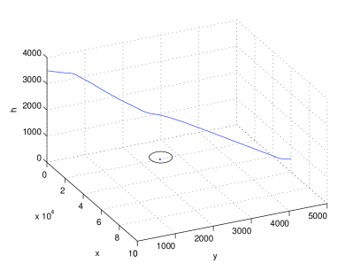
Figure 4. Trajectory in 3D

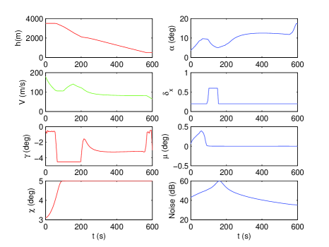
Figure 5. Solutions of $(OCP)_{2}$

We obtain approximately the same characteristic for the trajectory while the noise reduction is still significative.

4.2. Several observers fixed on the ground

We can generalize the processus of minimization for several observers. In this case, we minimize the maximum of noise corresponding to several observers.
The problem to solve is written as follows :

(6) $$\quad(OCP)_{3}\left\{\begin{array}[]{l}\min\vartheta\\ \vartheta>=J_{{obs}_{j}}\\ \dot{z}(t)=f(z(t),u(t))\\ z_{I_{1}}(0)=c_{1},\,z_{I_{2}}(t_{f})=c_{2}\\ \end{array}\right.$$

where $J_{{obs}_{j}}$ are the noise levels corresponding to $j$ fixed observers.

Once again, we use a direct method to solve the problem $(OCP)_{3}$ with the same modeling language and software.
We choose five observers : $(obs_{1}(0,0)$, $obs_{2}(20000,2500)$, $obs_{3}(40000,5000)$,
$obs_{4}(60000,0)$, $obs_{5}(60000,5000))$ which represent a certain area near the airport. We obtained an optimal solution, the obtained noise level is $49.65$ dB, the accuracy of the results is still very high $(max(f.o,e.o)=5.89e-07)$ and the algorithm takes no more $130s$ on a standard PC. This trajectory is about 5 dB less that $J_{1}(54.18$ dB).
The trajectory characteristics are given in the following figures:

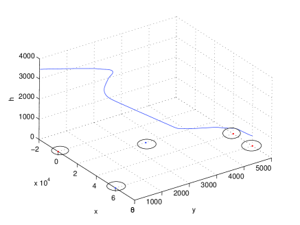
Figure 6. Trajectory in 3D with several observers

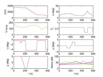
Figure 7. Solutions of $(OCP)_{3}$

Almost all state and control variables (except $\alpha$ and $V$) present large constant stages. The control variables $\delta_{x}$ and $\mu$ are bang-bang between their prescribed bounds.

5. Conclusion

We have performed a numerical computation of the optimal control issue. An optimal solution of the discretized problem is found with a very high accuracy. A noise reduction is obtained during the phase approach by considering the configuration of one and several observers. The trajectory obtained presents interesting characteristics and performances.

Extensions of the analysis on the current problem should include other source of noise. This feature is particularly important since improved noise model that better represent individual noise sources (engines, airframe,…). It should be remembered that this model is focused on single event flight. Additional researches are needed to fully assess the influence of wind and other atmospheric conditions on noise prediction process. The noise studies have, as yet, been limited to a single aircraft type equipped with two engines. Further research should consider multiple flights model considering airport capacity and nearby configuration.

Acknowledgments

We would like to thank Thomas Haberkorn for his constructive comments and his valuable help and suggestions for computational aspects.

References

- [1] L. Abdallah Minimisation des bruits des avions commerciaux sous contraintes physiques et a rodynamiques, PhD. thesis, Claude Bernard University, 2007.
- [2] AMPL A Modeling Language for Mathematical Programming, http://www.ampl.com
- [3] N. Berend, F. Bonnans, M. Haddou, J. Varin, C. Talbot An Interior-Point Approach to trajectory Optimization, INRIA Report, N. 5613, 2005.
- [4] A.Bolonkin and K.Narenda Method for finding a global minimum. AIAA-94-4420, Jan. 1994.
- [5] P.T.Boggs and J.W.Tolle Sequential Quadratic Programing. Acta numerica, pp. 1-52, 1995 .
- [6] J.Boiffier The Dynamics of Flight. John Wiley and Sons, 1998.
- [7] R. H. Byrd, J. Nocedal, and R. A. Waltz KNITRO: An Integrated Package for Nonlinear Optimization, 2006. http://www-neos.mcs.anl.gov/neos/solvers
- [8] G.Gilyard and A.Bolonkin Optimal pitch thrust-vector angle and benefits for all flight regimes. NASA Report, NASA/TM-2000-209021, 2000
- [9] ICAO. Environmental protection. Annex 16 to the Convention on International Civil Aviation. Aircrfat Noise, 1, 1993.
- [10] ICAO. Technical manual for environment specified the usage of methods for aircraft noise certification. Doc. 9501, Montreal, 1995.
- [11] S. Jonkhart A study into existing methodologies for the calculation of noise exposure levels and around airports. National Aerospace Laboratory Report NLR CR 92515 L, 1992.
- [12] J. Lambert and M. Vallet Study related to the preparation of a communication on a future EC noise policy. LEN, Final Report, No. 9420, Paris, 1994.
- [13] J. D. Mattingly Elements of Gas Turbine Propulsion, McGraw-Hill, 1996
- [14] B. W. McCormick Aerodynamics, Aeronautics and Flight Mechanics. John Wiley & Sons, NY, 1979.
- [15] L. Montrone Comparison of aircraft noise computation methods in Europe. National Aerospace Laboratory, NLR /NLR-CR-2000-055, 2000.
- [16] F. Miyara, S. Gabanellas, P. Mosconi, V. Pach, M. Yamtelli, J. C. Rall and J. Vazquez The acoustical geometry of aircraft oberflights. The 2001 International Congress and Exihibition on Noise control Engineering. The Hague, The Nether lands, pp. 27-30, 2001.
- [17] T. D. Norum and M. C. Brown Simulated High-Speed Flight Effects on Supersonic Jet Noise. AIAA Paper 93-4388, 1993.
- [18] S. J. Pietrzko and R. F. Hofmann Mathematical modelling of aircraft noise based on identified directivity patterns. American Institute of Aeronautics and Astronautics. AIAA 96-1768, pp. 1-14, 1996.
- [19] N. Rajan and M. D. Ardema Interception in Three Dimensions: An Energy Formulation. J. Guidance, Vol. 8, No. 1, 1985.
- [20] W. M. Schuller, F. D. van der Ploeg, and P. Bouter Impact of diversity in aircraft noise rating. J. Noise Control Eng, Vol. 43 (6), pp. 209-215, 1995.
- [21] J. P. Smith, R. A. Burdisso, C. R. Fuller and R. G. Gibson Active control of low-frequency broadband jet engine exhaust noise. Noise Control Engineering Journal, Vol. 44, No. 1, pp. 45-58, 1996.
- [22] J. R. Stone, D. E. Groesbeck and L. Zola Charles An improved prediction method for noise generated by conventional profil coaxial jets. National Aeronautics and Space Administration. Report NASA-TM-82712, AIAA-1991, 1981.
- [23] C. K. W. Tam Computational Aeroacoustics: Issues and methods. AIAA Journal, vol. 33, pp. 1788-1796, 1995.
- [24] C. K. W. Tam Supersonic Jet Noise. Annu. Review Fluid Mech., Vol. 27, pp. 17-43, 1995.
- [25] C. K. W. Tam and L. Auriault Jet Mixing Noise from Fine-Scale Turbulence. J. AIAA, Vol. 37, N. 2, pp. 145-153, 1999.
- [26] C. K. W. Tam Noise from High Speed Jets. Lecture Notes. VKI Lecture series on Advanced in Aeroacoustics. Lecture Series 2001 - 2002, Ed. by J. Anthoine and C. Schram, pp. 1, 34, 2001.
- [27] V. I. Tokarev, O. I. Zaporozhets and M. Valery Vorotyntsev : Sound Generation by Airborne Air Conditioning Systems: Theory and Analysis. Applied Acoustics, Vol. 55, No. 2, 1998.
- [28] S. Wright Interior-point methods for optimal control of discrete-time systems, J. Optim. Theory Appls, Vol. 77, pp. 161-187.
- [29] O. I. Zaporozhets and V. I. Tokarev Aircraft Noise Modelling for Environmental Assessment Around Airports. Applied Acoustics, Vol. 55, No. 2, pp. 99-127, 1998
- [30] O. I. Zaporozhets and V. I. Tokarev Predicted Flight Procedures for Minimum Noise Impact. Applied Acoustics, Vol. 55, No. 2, pp. 129-143, 1998
- [31] O.I.Zaporozhets and S.Khardi Optimisation of aircraft flight trajectories as a basis for noise abatement procedures around the airports. Theoretical considerations and acoustical applications. INRETS Report. N. 257, 2004