Warming the early Earth - CO₂ reconsidered

Abstract

Despite a fainter Sun, the surface of the early Earth was mostly ice-free. Proposed solutions to this so-called ”faint young Sun problem” have usually involved higher amounts of greenhouse gases than present in the modern-day atmosphere. However, geological evidence seemed to indicate that the atmospheric CO₂ concentrations during the Archaean and Proterozoic were far too low to keep the surface from freezing. With a radiative-convective model including new, updated thermal absorption coefficients, we found that the amount of CO₂ necessary to obtain 273 K at the surface is reduced up to an order of magnitude compared to previous studies. For the late Archaean and early Proterozoic period of the Earth, we calculate that CO₂ partial pressures of only about 2.9 mb are required to keep its surface from freezing which is compatible with the amount inferred from sediment studies. This conclusion was not significantly changed when we varied model parameters such as relative humidity or surface albedo, obtaining CO₂ partial pressures for the late Archaean between 1.5 and 5.5 mb. Thus, the contradiction between sediment data and model results disappears for the late Archaean and early Proterozoic.

, , , , , , and

1 Introduction

Geological evidence has shown that liquid water was present on the Earth’s surface earlier than 3.7 Gy ago (e.g., Mojzsis et al., 1996; Rosing and Frei, 2004) which implies average temperatures on the surface above 273 K. Some authors have even argued for a hot Archaean climate ($T$ $>$340 K), based on oxygen (Knauth and Lowe, 2003) and silicon (Robert and Chaussidon, 2006) isotope analysis of seawater cherts. However, as pointed out by, e.g., Kasting and Howard (2006) and Shields and Kasting (2007), these isotopic signatures changes might not only be caused by temperature effects. Sleep and Hessler (2006), for example, deduced a more moderate surface temperature below 300 K, based on quartz weathering records in paleosols. Nevertheless, it is generally accepted that the Earth has been ice-free throughout most of its history.

Observations of several solar-type stars of different ages and virtually all standard models of the solar interior have shown that the total solar luminosity has increased since the ZAMS (Zero Age Main Sequence) by about 30% (Gough, 1981; Caldeira and Kasting, 1992). Had the composition of the Earth’s atmosphere been the same then as today, the reduced solar flux would have resulted in surface temperatures below 273 K prior to 2.0 Gy (Sagan and Mullen, 1972). This apparent contradiction between solar evolution models, climatic simulations and geological evidence for liquid water and moderately warm temperatures on Earth has been termed the ”faint young Sun problem”.

Numerous studies have attempted to solve this problem. For example, Minton and Malhotra (2007) explored the hot early Sun scenario for a non-standard solar evolution. Shaviv (2003) showed that moderate greenhouse warming in combination with the influence of solar wind and cosmic rays on climate could resolve the problem. Jenkins (2000) assumed high obliquities in a General Circulation Model to account for high Archaean temperatures.

However, the most accepted scenario involves a much enhanced greenhouse effect (GHE) on the early Earth compared to modern Earth. Today, the GHE produces around 30 K of warming, raising the mean surface temperature of the Earth to about 288 K. Increased abundances of greenhouse gases such as carbon dioxide (Kasting, 1987), methane (Pavlov et al., 2000), ethane (Haqq-Misra et al., 2008) or ammonia (Sagan and Mullen, 1972; Sagan and Chyba, 1997) will strengthen the GHE, hence potentially resolve the problem. However, all of these studies faced some form of contradictions or large uncertainties, either from geological data on atmospheric conditions or from atmospheric modeling. The formation and destruction of ammonia is highly dependent on UV levels in the atmosphere (Sagan and Chyba, 1997; Pavlov et al., 2001). The hydrocarbon haze necessary to allow higher hydrocarbons to accumulate in the atmosphere depends critically on the CO₂/CH₄ ratio (Pavlov et al., 2003). The high values of methane required to heat the surface of the early Earth depend on estimates of the early biosphere and volcanic activity, which is not well determined. Past CO₂ concentrations required by atmospheric models (Kasting, 1987) to reach surface temperatures above 273 K are in conflict with inferred concentrations from the sediment data (Hessler et al., 2004; Rye et al., 1995).

In this work, the role of CO₂ in warming the early Earth is reconsidered. We used a one-dimensional radiative-convective model, including updated absorption coefficients in its radiation scheme for thermal radiation. The model was applied to the atmosphere of the early Earth in order to investigate the effect of enhanced carbon dioxide on its climate. Additionally, we investigated the effect of two important parameters, namely the surface albedo and the relative humidity, upon the resulting surface temperature.

Our results imply that the amount of CO₂ needed to warm the surface of early Earth might have been over-estimated by previous studies. Furthermore, the results show that the contradiction between modelled CO₂ concentrations and measured values might disappear by the end of the Archaean.

Section 2 describes the model and section 3 the runs to validate the new radiation scheme. The runs performed for this work are explained and summarized in section 4. In section 5, the results are presented and discussed. Section 6 gives the summary of the results.

2 Atmospheric Model

We used a one-dimensional radiative-convective model based on the climate part of the model used by Segura et al. (2003) and Grenfell et al. (2007a, b). Our model differs in upgrades of the radiation scheme to calculate the thermal emission in the atmosphere. The model calculates globally, diurnally-averaged atmospheric temperature and water profiles for cloud-free conditions. We will first state some basic characteristics of the model (2.1). Then we will describe the calculation of the energy transport via radiative transfer (solar and thermal fluxes) and convection (2.2) to obtain the atmospheric temperature profile. Thereafter, a description of the determination of the water profile is given (2.3). Finally, the model input parameters are summarized (2.4).

2.1 Basic model description

The model determines the temperature profile by assuming two dominant mechanisms of energy transport, i.e. radiative transfer and convection. The convective lapse rate is assumed to be adiabatic. The radiative lapse rate is calculated from contributions of both solar and thermal radiation, including Rayleigh scattering for solar radiation and continuum absorption in the thermal region. Table 1 summarizes the contributions of the different atmospheric species to the calculation of the temperature profile.

The species considered in the model are molecular nitrogen, water, molecular oxygen, argon, carbon dioxide and carbon monoxide. For example, a typical early Earth run considered 0.77 bar of nitrogen and several (2.9 - 57.2) mb of carbon dioxide in addition to water in varying concentrations (0.5—1 % at the surface). Molecular nitrogen is an effective Rayleigh scatterer (although not as effective as carbon dioxide) and as a main constituent of the atmosphere also contributes to the heat capacity. Water is not considered to be an important Rayleigh scatterer, but it is relevant for the other radiative processes. Also, water influences the adiabatic lapse rate because it readily condenses in the troposphere. However, due to small mixing ratios, especially in the stratosphere, water vapour does not contribute to the heat capacity of the atmosphere. Molecular oxygen and argon do contribute to the heat capacity of the atmosphere, and molecular oxygen additionally contributes to the Rayleigh scattering coefficient. Carbon dioxide contributes to all relevant radiative mechanisms (molecular absorption of solar and thermal radiation, continuum absorption, Rayleigh scattering), but not to the adiabatic lapse rate because it does not condense under conditions described in this paper. Carbon monoxide is an important absorber species in some mid-infrared windows and contributes to the heat capacity.

The model assumes the hydrostatic relation between pressure $p$ and density $\varrho$ throughout the plane-parallel atmosphere. On the 52 model layers, a logarithmic pressure grid is calculated. Specified pressure levels at the planetary surface (e.g., 1 bar for the standard Earth case) and the upper model lid (at 6.6$\cdot 10^{-5}$ bar) determine the altitude range which, for modern Earth conditions, extends to 65-70 km, i.e. the lower- to mid mesosphere. For all gases except water, the ideal gas law is taken as the equation of state (see 2.2.4 for water). The effect of clouds is difficult to incorporate into 1D models (see, for example, Pavlov et al., 2000; Segura et al., 2003). In the present model, following the approach of Segura et al. (2003), clouds are implicitly included by adjusting the surface albedo $A_{\rm{surf}}$ such that under modern Earth control conditions the model calculates a mean surface temperature of 288 K. The required value for $A_{\rm{surf}}$ is about 0.21, whereas the actual global value for Earth is approximately 0.15. This can be interpreted as a ground cloud layer instead of tropospheric or stratospheric clouds. The model uses a time-stepping algorithm to convergence to the steady-state solution(Pavlov et al., 2000).

2.2 Temperature profile

During each time step, the temperature profile is calculated from the radiative equilibrium condition. The temperature $T$ on an atmospheric level $z$ is determined by the following equation of energy conservation (Pavlov et al., 2000):

$$\frac{d}{dt}T(z)=-\frac{g}{c_{p}(T,z)}\frac{dF(z)}{dp(z)}$$ (1)

where $dt$ is the time step in the model, $c_{p}$ the heat capacity, $F$ the total net radiative flux and $p$ the pressure of the level. The radiative flux $F$ is the sum of thermal planetary and atmospheric emission, $F_{\rm{thermal}}$, and the solar radiative input, $F_{\rm{solar}}$, into the atmosphere:

$$F(z)=F_{\rm{thermal}}(z)+F_{\rm{solar}}(z)$$ (2)

These fluxes are calculated separately by two numerical schemes which solve the monochromatic radiative transfer equation (RTE) for the spectral intensity $I_{\nu}$ in the respective spectral domain (i.e., near-UV to near-IR for solar flux, near-IR to far-IR for thermal flux):

$$\mu\frac{dI_{\nu}}{d\tau_{\nu}}=I_{\nu}-S_{\nu}$$ (3)

where $S_{\nu}$ is the source function (either the incident solar radiation or the thermal blackbody emission of the atmospheric layers and the planetary surface), $d\tau_{\nu}$ the optical depth and $\mu=\cos(\theta)$ the cosine of the polar angle. The optical depth is defined as usual by

$$d\tau=-(\kappa_{\nu}+s_{\nu})dz$$ (4)

where $\kappa_{\nu}$ and $s_{\nu}$ represent the absorption coefficient and the scattering coefficient respectively. The absorption coefficient for a gas mixture is calculated from the individual absorption coefficients of the gas species $i$:

$$\kappa_{\nu}=\sum_{i}\kappa_{\nu,i}=\sum_{i}\sigma_{\rm{abs},i}\cdot N_{i}$$ (5)

where $N_{i}$ is the number density and $\sigma_{abs,i}$ the molecular absorption cross section of the gas species $i$. When no scattering occurs (i.e., $s_{\nu}=0$), eq. 4 can be written in terms of the column density $W_{i}$ of the gas species $i$ as:

$$\tau=\sum_{i}\sigma_{\rm{abs},i}\cdot W_{i}$$ (6)

The absorption cross section is defined by:

$$\sigma_{\rm{abs}}(\nu,p,T)=\sum_{j}S_{j}(T)\cdot g_{j}(\nu,T,p)$$ (7)

Here, $S_{j}(T)$ is the temperature-dependent line strength of a particular spectral line $j$ and $g_{j}(\nu,T,p)$ the temperature- and pressure-dependent line shape function of the same line.

For the scattering coefficient, an analogous equation is valid:

$$s_{\nu}=\sum_{i}s_{\nu,i}=\sum_{i}\sigma_{y,i}(\nu)\cdot N_{i}$$ (8)

Here, $\sigma_{y,i}(\nu)$ is a scattering cross section of type $y$. In the present model, Rayleigh scattering is considered.

The solution of eq. (4), i.e. the calculation of optical depths, is one of the key elements in radiative-convective models. This solution, of course, depends on the accurate calculation of the absorption cross sections.

From eq. (3), the necessary fluxes for eq. (2) (i.e., the thermal and the solar flux) are obtained by an angular integration of the (monochromatic) intensity:

$$F_{\nu}=\int_{\Omega}d\omega\mu I_{\nu}$$ (9)

and a frequency integration of the (monochromatic) flux:

$$F_{\nu_{1}\rightarrow\nu_{2}}=\int_{\nu_{1}}^{{\nu_{2}}}F_{\nu}d\nu$$ (10)

Each one of these integrations is performed independently for the two components of the total flux.

2.2.1 Solar radiation

The solar radiation module which calculates $F_{\rm{solar}}(z)$ for eq. (2) has already been used by, e.g., Pavlov et al. (2000); Segura et al. (2003) or Grenfell et al. (2007a) and is based on Kasting et al. (1984b) and Kasting (1988). The module considers a spectral range from 0.26 to 4.5 $\mu$m in 38 intervals. It evaluates the solar incident radiation at a fixed daytime average solar zenith angle of 60^∘. Contributions to the optical depth come from gaseous absorption by water and carbon dioxide (i.e., $\kappa_{\nu}$ in eq. (4)) and from Rayleigh scattering by carbon dioxide, molecular nitrogen and molecular oxygen (i.e., $s_{\nu}$ in eq. (4)).

Absorption cross sections $\sigma_{\rm{abs}}$ for the solar code were obtained from the HITRAN 1992 database (Rothman et al., 1992). Rayleigh scattering cross sections $\sigma_{ray}$ are parameterized following Vardavas and Carver (1984). The frequency integration (see also eq. (10)) of the RTE for $F_{solar}$ in each of the 38 spectral intervals is parameterized by a four-term correlated-k exponential sum (e.g., Wiscombe and Evans, 1977). The following angular integration (eq. (9)) is performed by using a quadrature $\delta$-2-stream approximation code based on Toon et al. (1989). The resulting fluxes from each spectral interval are added up to yield the total solar flux $F_{\rm{solar}}(z)$ at an atmospheric level $z$. This flux is further multiplied by a factor of 0.5 to account for diurnal variation.

2.2.2 Thermal molecular absorption

The thermal (planetary) radiation module for $F_{\rm{thermal}}(z)$ in eq. (2) considers a spectral range from 1 to 500 $\mu$m in 25 intervals. Our new thermal module is called MRAC (Modified RRTM for Application in CO₂-dominated Atmospheres) and is based on the radiation scheme RRTM (Rapid Radiative Transfer Model). RRTM was developed by Mlawer et al. (1997) and has been used by numerous other modeling studies (e.g., Segura et al., 2003, 2005; Grenfell et al., 2007a, b). The need for a new radiation model comes from the fact that RRTM was specifically designed for conditions of modern Earth, i.e. it is not adaptable to studies of atmospheres which greatly differ from modern atmospheric conditions (in terms of atmospheric composition, temperature structure, pressure, etc.). MRAC is easily adaptable to varying conditions, as is described below.

MRAC uses the correlated-$k$ approach (e.g., Goody et al., 1989; Lacis and Oinas, 1991; Colaprete and Toon, 2003) for the frequency integration of the RTE in the thermal range, as does RRTM. The planetary surface (bottom layer of the model atmosphere) and the atmospheric layers are taken as blackbody emitters, according to their respective temperatures. The thermal surface emissivity is set to unity. The absorber species considered in MRAC are water, carbon dioxide and carbon monoxide. The angular integration (eq. (9)) is performed using the diffusivity approximation (as in Mlawer et al., 1997).

The correlated-k method

Basically, this method transfers the frequency integration (FI) of the RTE from frequency space $\nu$ to a probability space $g$. For the absorption cross section $\sigma_{\rm{abs}}$ of eq. (7) in an interval $[\nu_{1},\nu_{2}]$, a probabilistic density distribution $f(\sigma_{\rm{abs}})$ (i.e., probability of occurence for a particular value of $\sigma_{\rm{abs}}$) with the following normalization condition can be defined:

$$\int_{0}^{{\infty}}f(\sigma_{\rm{abs}})d\sigma_{\rm{abs}}=1$$ (11)

To follow conventional nomenclature in the literature regarding $k$-distributions, $\sigma_{\rm{abs}}$ is hereafter referred to as $k$. The function $f(\sigma_{\rm{abs}})=f(k)$ is called the $k$-distribution. From the $k$-distribution, a cumulative $k$-distribution $g(k)$ can be defined by

$$g(k)=\int_{0}^{{k}}f(k^{\prime})dk^{\prime}$$ (12)

The cumulative $k$-distribution is a strictly monotonic function and may thus be inverted from $g(k)$ to yield $k(g)$. This mapping of the frequency information ($k(\nu)$) into a single probability variable ($k(g)$) can be done because it is irrelevant at which position of the spectral interval a particular value of the absorption cross section $k$ occurs. Performing a variable substitution in eq. (10) then leads to the following equation:

$$F_{\nu_{1}\rightarrow\nu_{2}}=\int_{\nu_{1}}^{{\nu_{2}}}F(\nu)d\nu=\int_{0}^{{1}}F(g)dg$$ (13)

The goal of the cumulative-$k$ approach is to reduce the number of radiative transfer operations drastically while keeping the accuracy of line-by-line models. This can be achieved with very few numbers of points in $g$ space (see Goody et al., 1989; West et al., 1990). The $g$ integration in eq. (13) is performed in MRAC by Gaussian quadrature using 16 intervals in $g$ space (the same as used in RRTM, Mlawer et al., 1997).

The extension of this exact method from homogeneous to inhomogeneous atmospheres is called the correlated-$k$ method (e.g., Mlawer et al., 1997). Each $g$ interval is treated as if it were a monochromatic frequency interval, i.e. the method uses the same subset of $g$ space for all layers throughout the atmosphere. This implies a full frequency correlation of a specific subset of $g$ space for all atmospheric layers. There are conditions under which this approach is exact (Goody and Yung, 1989), but usually these do not hold. However, the numerical error of the correlated-$k$ method is generally small (Mlawer et al., 1997).

Creating the new radiation scheme

MRAC was originally designed to simulate atmospheres of a wide range of possible terrestrial planets other than modern Earth, as stated above. Therefore, a new temperature-pressure ($T$-$p$) grid to incorporate the aforementioned ($T$,$p$)-dependence of the absorption cross sections (see eq. 7) has been introduced. In RRTM, $k$ values are tabulated for every spectral band and every point in $g$ space for 59 pressure levels and the associated Mid-Latitude-Summer (MLS) standard Earth temperature values as well as temperature values T${}_{\rm{MLS}}\pm$ 15 K and T${}_{\rm{MLS}}\pm$ 30 K, as described in Mlawer et al. (1997). The $T$-$p$ grid of RRTM is thus more or less fixed to modern Earth conditions. For MRAC, we used 8 pressure levels, ranging equidistantly in log $p$ from 10^-5 to 100 bar and 9 temperature points, 6 in 50 K steps from 150 K to 400 K and three additional points for 500, 600, 700 K respectively. Tests showed that this grid allows for an interpolation accuracy of usually better than 2-3%. Furthermore, the number of $T$-$p$ points is consistent with previous modeling studies (Kasting et al., 1993; Colaprete and Toon, 2003).
Figure 1 shows the range of the tabulated $k$-values for both RRTM and MRAC, i.e. the interpolation regime of the two radiative schemes. It demonstrates that RRTM can only be applied to a much narrower range of atmospheric conditions in comparison to MRAC.

The necessary re-calculation of the $k$-distributions for each of the gases included in MRAC (water, carbon dioxide, carbon monoxide) proceeded in three steps:

First, the absorption cross sections for every species were calculated for each $T$-$p$ grid point in each of the spectral intervals where the respective species is active. The line shape cut-off was set to 10 cm^-1 from the frequency $\nu$, i.e. the sum over $j$ in eq. (7) contains contributions from all lines within $\pm$ 10 cm^-1. For the line shape $g_{j}(\nu,T,p)$, a Voigt profile was assumed. The required line parameters were taken from the HiTemp 1995 database (Rothman et al., 1995). The foreign broadening parameters in HiTemp are given for air, i.e. an oxygen-nitrogen mixture as a background atmosphere. However, as reported by several authors (e.g., Brown et al., 2005; Toth, 2000), the foreign broadening parameters vary by significant amounts when different broadening gases are considered. Thus, for each type of background atmosphere, a new set of $k$-distributions must be generated (e.g., low-oxygen atmospheres, CO₂-dominated atmospheres, intermediate N₂-O₂-atmospheres). These line parameters were then used as input to a line-by-line radiative transfer model called Mirart (Schreier and Böttger, 2003). Mirart produced the actual absorption cross sections with a spectral resolution of 10⁶ equidistant points per spectral interval.

Second, the $k$-distributions $f(k)$ were calculated from the absorption cross sections. From the $k$ distribution $f(k)$, the cumulative $k$-distribution $g(k)$ was then obtained.

Third, representative $k$ values were calculated for each of the $g$ subintervals. In this step, our algorithm followed the approach of Mlawer et al. (1997), i.e. for each of the 16 Gaussian subintervals in $g$ space, an arithmetic mean absorption cross section was calculated.

MRAC also implements a so-called binary species parameter $\eta$ for transmittance calculations. This is employed in intervals having two important absorber species (for more details, see Mlawer et al., 1997 or Colaprete and Toon, 2003):

$$\eta=\frac{C_{1}}{C_{1}+r\cdot C_{2}}$$ (14)

Here, $C_{1,2}$ are the concentrations of the two gases (in the case of MRAC, water and carbon dioxide) and $r$ is some specified reference ratio (mean modern Earth tropospheric values). Carbon monoxide, although present in the model in six spectral intervals, is not considered to be part of the binary species parameter. This is partly due to the expected low concentrations in the simulated atmospheres (typical theoretical and measured values for early Earth and Mars are below 10^-4 volume mixing ratio), partly due to the expected low temperatures (below 300 K), which means that the strong CO fundamentals around 4 $\mu$m are completely outside the relevant Planck emission windows. Consequently, carbon monoxide has only a reduced impact on the radiation budget, compared to water and carbon dioxide. $k$-distributions are calculated in MRAC for 5 different values of $\eta$, ranging equidistantly from 0 (CO₂ only) to 1 (H₂O only).

Another improvement in MRAC, compared to RRTM, is the treatment of the Planck function in each band. The fraction of thermal radiance associated with a subset in $g$ space is calculated from eq. (11) in Mlawer et al. (1997):

$$f_{g}=\frac{B_{g}w_{g}}{\overline{B}_{g}}$$ (15)

Here, $B_{g}$ is the average Planck function of the frequencies in the subset of $g$ space, $w_{g}$ the Gaussian weight of the $g$ interval and $\overline{B}_{g}$ the average Planck function of the whole spectral band (i.e., the whole $g$ space). As temperature, pressure and species concentrations vary, the different $g$ subsets will correspond to different frequencies, and as such the value of $B_{g}$, thus $f_{g}$, will vary. This has been taken into account while constructing the $k$-distributions.

Mlawer et al. (1997) tabulated values of $f_{g}$ for every value of the binary species parameter and for two atmospheric reference levels, one each in the troposphere and the stratosphere. In MRAC, values of $f_{g}$ were tabulated for three temperatures and two pressure levels as well as for the values of the binary species parameter. The most important factor for $f_{g}$ is the binary species parameter $\eta$, whereas the variation with temperature and pressure is rather small, although not negligible. Therefore these 6 $T$-$p$ points are regarded as to be sufficient.

A further difference between RRTM and MRAC is the distinction between troposphere and stratosphere. In the troposphere, RRTM changes major and minor absorbers in some of the spectral intervals (see table 1 in Mlawer et al., 1997). In some spectral bands, no absorption is considered in the stratosphere, in others, the number of key species is reduced. This is done because on Earth, the chemical and physical regimes are quite different in the troposphere compared to those in the stratosphere. However, as this is mostly due to Earth-specific conditions (e.g., the cold trap, tropopause and temperature inversion all approximately occur at the same altitude), this distinction was not incorporated into MRAC.

2.2.3 Thermal continuum absorption

Based on approximation formulations used by Kasting et al. (1984b), Kasting et al. (1984a) and Colaprete and Toon (2003), additional CO₂ and H₂O continuum absorption in the thermal region is considered. In contrast, the RRTM scheme only considers water continuum absorption (Mlawer et al., 1997).

Equation (16) shows the approximation for the optical depth $\tau_{\rm{cont},\rm{CO_{2}}}$ due to CO₂ continuum absorption. The corresponding parameters are taken from Kasting et al. (1984b).

$$\tau_{\rm{cont},\rm{CO_{2}}}=C_{i}W\cdot p_{E}\left(\frac{T_{0}}{T}\right)^{t_{i}}$$ (16)

In this equation, $C_{i}$ a frequency-dependent adjustment to the path length, $W$ the column amount of CO₂, $p_{E}=(1+0.3\cdot C_{\rm{CO_{2}}})\cdot p$ ($p$ layer pressure, $C_{\rm{CO_{2}}}$ concentration) an effective CO₂ broadening pressure and $T_{0}$=300 K is a reference temperature.

The optical depth $\tau_{\rm{cont},\rm{H_{2}O}}$ due to water continuum absorption in the window region (8-12 $\mu$m) is calculated from the equation (Kasting et al., 1984a)

$$\tau_{\rm{cont},\rm{H_{2}O}}=h_{n}\cdot p\cdot\frac{W_{w}^{2}}{W_{t}}$$ (17)

where $h_{n}=h_{t}\cdot h_{\nu}$ incorporates the frequency and temperature dependence, $p$ is the pressure, $W_{t}$ the total and $W_{w}$ the water column of the layer. $h_{\nu}$ is evaluated at the high frequency interval boundary, as in Kasting et al. (1984a). We use the following approximations for $h_{t}$ and $h_{\nu}$, based on Kasting et al. (1984a) and Colaprete and Toon (2003):

$$h_{t}=e^{1800\cdot(\frac{1}{T}-\frac{1}{296})}$$ (18)

$$h_{\nu}=1.25\cdot 10^{-22}+1.67\cdot 10^{-19}\cdot e^{-2.62\cdot 10^{-13}\cdot\nu}$$ (19)

Both the water and the carbon dioxide continuum absorption are considered to be approximately monochromatic over a specific spectral interval, hence their contribution to the overall absorption coefficient (see eq. (4)) is added as a constant term.

2.2.4 Convective adjustment

Convective adjustment to the lapse rate is performed whenever the calculated radiative lapse rate $\nabla_{\rm{rad}}T$ exceeds the adiabatic value $\nabla_{\rm{ad}}T$ (Schwarzschild criterion):

$$\nabla_{\rm{rad}}T>\nabla_{\rm{ad}}T$$ (20)

The adiabatic lapse rate is calculated as a standard dry adiabat in the stratosphere. In the troposphere, a wet H₂O adiabatic lapse rate is assumed. Below 273 K, the Clausius-Clapeyron-equation $\frac{d\ln(p_{v})}{d\ln(T)}=\frac{m\cdot L}{R\cdot T}$ ($R$ universal gas constant, $m$ mass, $L$ latent heat release per mass) for the saturation vapor pressure curve $p_{v}$ is applied. Between 273 and 647 K, a formulation by Ingersoll (1969) is taken.

2.3 Atmospheric water profile

In every time step, the water vapor profile is re-calculated according to the new temperature profile.

In the troposphere, water vapor concentrations $C_{\rm{H_{2}O}}$ are calculated from a fixed relative humidity distribution $RH$:

$$C_{\rm{H_{2}O}}(T,z)=\frac{p_{\rm{sat}}(T(z))}{p(z)}\cdot RH(z)$$ (21)

where $p_{\rm{sat}}$ is the saturation vapor pressure of water at the given temperature $T$ and $p$ the atmospheric pressure at level $z$. The default relative humidity profile $RH$ follows the approach of Manabe and Wetherald (1967), with a relative humidity $R_{s}$ of 80% at the surface.

$$RH(z)=R_{s}\cdot\frac{\frac{p(z)}{p_{\rm{surface}}}-0.02}{0.98}$$ (22)

Above the cold trap, water vapor is treated as a non-condensable gas, and its concentration is fixed at the cold trap value.

2.4 Boundary conditions, initial values and parameters

Since eq. (1) is a first order differential equation for the temperature, a starting temperature profile must be provided. In addition, a boundary condition for the radiative flux must be specified. To obtain unique equilibrium solutions, parameters must also be provided for the model. These include pressure parameters for the planetary top-of-atmosphere (TOA) pressure $p_{0}$, gas concentrations, surface albedo or solar zenith angle, for example.

Table 2 summarizes the boundary conditions, initial values and parameters.

3 Validation of the new radiation scheme

3.1 General remarks

MRAC has been tested in two different ways.

• Case 1: $k$-distributions
  The calculated $k$-distributions, i.e. the model input data, have been validated against published values to show that the algorithm creating the $k$-distributions works correctly.

• Case 2: Earth atmosphere temperature profiles
  Temperature profiles of an Earth-like test atmospheres (composition: N₂ 0.77, O₂ 0.21, Ar 0.01, CO₂ 3.55 $\cdot$ 10^-4) calculated with MRAC and RRTM have been compared. This was done since RRTM has been extensively validated both against line-by-line codes and atmospheric measurements (Mlawer et al., 1997) under modern Earth conditions.

  Our test atmosphere has a composition close to the present day atmosphere. However, it lacks radiative trace gases such as nitrous oxide, ozone and methane, as these gases cannot be handled by MRAC yet (see above). Note that due to the lack of ozone in our test atmosphere, we do not expect a large stratospheric temperature maximum as is observed in the present Earth atmosphere because this maximum is almost entirely due to the absorption of solar radiation by ozone.

  We additionally performed test runs on a second test atmosphere (not shown) which differs from the first one by its CO₂ content (100-fold increase). This 100-fold increase in CO₂ represents the current limit for the RRTM scheme (Segura et al., 2003, Eli Mlawer, priv. comm.).

These two validation approaches are discussed below.

3.2 $k$-distributions

Figures 2 and 3 compare our calculated $k$-distributions (dotted lines) with previously published values (plain lines) for different water and carbon dioxide bands. Published values were taken from Lacis and Oinas (1991) (H₂O, Fig. 2) and Mlawer et al. (1997) (CO₂, Fig. 3). Figures 2 and 3 indicate quite good agreement with the published values.

3.3 Earth temperature profiles

The calculated temperature profiles for the test atmosphere are shown in Fig. 4.

Figure 4 implies some differences in the middle to upper stratosphere (2-6 K) and small deviations ($\ll 1K$) below about 20 km. For the test atmosphere with a 100-fold increase in CO₂ (not shown), the stratospheric differences are even larger (up to 10 K). We interpret these differences in the temperature profiles as follows:

Firstly, as stated above in section 2.2.2, MRAC does not differentiate between troposphere and stratosphere, as is the case for RRTM. That means, spectral bands where H₂O or CO₂ absorb only weak are not considered for optical depth calculations in the stratosphere by RRTM (e.g., bands 6, 12-13 and 15-16). In contrast, MRAC incorporates the contribution of CO₂ and H₂O to the optical depth in these spectral bands. However, this contribution is usually rather small.

Secondly, and more importantly, the differences between the stratospheric temperature profiles occur where RRTM has to use a temperature extrapolation for the absorption cross sections beyond the limits of its tabulated values.

Fig. 5, shows the temperature profile for our test atmosphere Earth 1. Also shown is the validity range of RRTM as already indicated in Fig. 1. This represents the lower temperature limit for the tabulated absorption cross sections in RRTM, as stated above.

As can be seen from Fig. 5, the calculated temperature values for the first test atmosphere are below the lower RRTM validity limit. Therefore, RRTM uses linear extrapolation to calculate the absorption cross sections. This introduces a large extrapolation error. On average, the calculated absorption cross sections are a factor of 2-5 too low, depending on the spectral band. Sometimes, the extrapolation performed by RRTM even yields negative absorption cross sections. The interpolation errors in MRAC, on the contrary, reach only 1-2% on average.

Figure 6 shows the radiative fluxes and heating and cooling rates calculated by RRTM and MRAC in the test atmosphere Earth 1. Solar fluxes and heating rates differ by much less than 1 %. The thermal down-welling fluxes calculated by RRTM and MRAC show large differences in the stratosphere below pressures of around 10^-2-10^-3 bar, reaching up to a factor of 5 in the upper stratosphere where pressures are below 10^-4 bar. However, these differences are well below 1 W m^-2, so are not discernible on the scale in Figure 6. The up-welling fluxes differ by only about 10 % in the stratosphere, since they are dominated by the tropospheric component. Hence, the calculated resulting cooling rates differ only by small amounts of 0.1-0.4 K day^-1 and usually lie within 5-10 %, especially in the upper stratosphere.

In order to assess the sensitivity of the model to errors in the absorption cross sections (hence, in optical depth and thermal fluxes), we artificially increased the optical depth in RRTM in the most important stratospheric band, the CO₂ 15$\mu$m fundamental by factors of 2, 5, 10 and 20, respectively. Fig. 7 quantifies the effect of these sensitivity runs on the temperature profile. Fig. 7 a) shows the total optical depth calculated by RRTM and MRAC in the validation runs. Clearly, in the stratosphere, RRTM under-estimates the optical depth, as already discussed above.

Fig. 7 b) shows the temperature profiles for the two Earth validation runs with MRAC and RRTM, as well as for a run with RRTM, but increased optical depth by a factor of 2. This factor of 2 is representative of the error in the absorption cross section calculations in the 15 $\mu$m band due to the required extrapolation in the $T$-$p$-range, as shown in Figure 1. It can be seen that by increasing the optical depth in RRTM artificially, the temperature profile nearly reproduces the MRAC temperature profile.

These results show that conditions which differ too much from the Earth’s standard atmosphere seem to pose problems for RRTM. This limitation was already noted in some of the previous studies performed with RRTM. Clearly, due to the use of an expanded temperature range, MRAC performs better than RRTM in these atmospheres.

4 About the runs

4.1 Absorption cross sections

The absorption cross sections used in the runs performed for this work (summarized in Tables 3 and 4) were calculated assuming a N₂-CO₂-background atmosphere, consisting of 95% molecular nitrogen and 5% carbon dioxide. According to Kasting and Ackerman (1986) and Toth (2000), the foreign broadening coefficient for water is enhanced by a factor of 2 with respect to air for CO₂ as a broadening gas and by a factor of 1.2 for N₂ as a broadening gas. Similarly, for carbon dioxide the foreign broadening coefficient was enhanced by a factor of 1.3 when N₂ was the broadening gas (Kasting and Ackerman, 1986). Accounting for the appropriate mixing ratios then yields an effective enhancement factor by which the foreign broadening parameter from HiTemp was multiplied before use in the cross section calculations described above.

We compared the calculated cross sections of the assumed N₂-CO₂-atmosphere (95% nitrogen and 5% carbon dioxide) with cross sections for some major spectral bands corresponding to different background atmospheres, i.e. different CO₂ concentrations. These cross sections were obtained with the line-by-line radiative transfer model Mirart (Schreier and Böttger, 2003). The cross sections from the 95%-N₂-5%-CO₂-atmosphere agree within 5 % for most of the cases studied in this work, although for the runs with the lowest CO₂ concentrations, the agreement decreased to about 10 %.

4.2 Model runs

There were a total number of 12 nominal runs performed as shown in Table 3.

We assumed a constant background pressure of 0.77 bar N₂ with variable amounts of CO₂. Water vapour contents of the atmosphere were calculated as described in section 2.3. No other gases were present in the atmosphere, as in Kasting (1987). For several values of the solar constant ($S$=0.7, 0.75, 0.8, 0.85, 0.9 and 0.95 present-day value), we increased the CO₂ partial pressure until converged surface temperatures reached 273 K (runs 1-6) and 288 K (runs 7-12), respectively. This procedure is similar to what was done by Kasting (1987). The solar constant values were chosen as to loosely correspond to important events throughout the Earth’s history, such as the beginning of the main sequence life time of the Sun ($S$=0.70, 4.6 Gy ago), the end of the late heavy bombardment ($S$=0.75, 3.8 Gy ago), the rise of oxygenesis by cyanobacteria ($S$=0.80, 2.9 Gy ago), the first and the second oxidation event ($S$=0.85 and $S$=0.90, 2 and 1.3 Gy ago respectively) and the Cambrian explosion ($S$=0.95, 0.6 Gy ago). Assigning geological ages to the solar constants used in the model (see Table 3) is essential when comparing the calculated model CO₂ concentrations to the available data and constraints on carbon dioxide. In this work, we chose two approximations of the solar luminosity $S(t)$ with time. The first one is from Caldeira and Kasting (1992), the second approximation is from Gough (1981). The difference of these two formulations is most pronounced for earlier time periods before 1-2 Gy ago, although it is rarely larger than a few percent.

The total surface pressure is always calculated from the relation $p_{\rm{surf}}=p_{\rm{CO_{2}}}+p_{\rm{N_{2}}}+p_{\rm{H_{2}O}}$. Since we calculated surface temperatures of 273 K and 288 K, the amount of surface pressure which arose from the evaporation of water is about 6 mb and 17 mb, respectively. Note that the total surface pressure in our model runs decreases with time, as we assume less CO₂ partial pressure in our model atmospheres. There is no geological data available on the total surface pressure throughout time, however, our approach of constant N₂ partial pressure is consistent with assumptions made in previous studies (e.g., Kasting, 1987).

4.3 Parameter variations of surface albedo and relative humidity profile

Previous works regarding the ”faint young Sun problem” have concentrated on the increased greenhouse effect, as stated above in the Introduction. We also studied two important parameters affecting the surface temperature in our model, namely the surface albedo and the relative humidity (RH) distribution.

The importance of cloud coverage for the surface temperature, e.g. on early Mars, has been studied by Mischna et al. (2000). The effect in their model was quite large, yielding surface temperatures from 220 K to 290 K, depending on cloud optical depth and cloud location. In our model, the surface albedo simulates the presence of clouds, as stated above in the description of our model.

Water vapour is a very effective greenhouse gas. In contrast to CO₂, its content in the troposphere (where 99 % of the column resides) is controlled by the hydrological cycle (ocean reservoir, evaporation, subsequent condensation and precipitation) which is very sensitive to temperature. A critical parameter in climate models is the relative humidity parametrization, which clearly has a potentially large impact on the water content in the atmosphere and hence on the resulting greenhouse effect.

In addition to the model runs described above, we therefore performed runs varying surface albedo and relative humidity profiles. These runs are based on runs 3 and 4 of Table 3, i.e. solar constants of $S$=0.8 and $S$=0.85. Table 4 summarizes the parameter variations.

In the runs from Table 3, the surface albedo is normally set to $A$=0.21 (see Table 2). Now, we assume surface albedos of $A$ $\pm$10 %, i.e. 0.19 and 0.23, respectively.

The relative humidity profile used for the calculation of water vapour concentrations in Table 3 follows the approach of Manabe and Wetherald (1967) (referred to as RH=MW, see section 2.3). Here, for the additional parameter studies, we used three different RH profiles. The first one assumed a saturated troposphere (RH=1). The second profile used RH=0, i.e. water was removed from the atmosphere. These two profiles represent the lower and upper limits of the atmospheric water content. The third RH profile is a more realistic RH profile. It is based on a temperature correction to the RH profile of Manabe and Wetherald (1967) which was first proposed by Cess (1976) and later used by Vardavas and Carver (1985).:

$$R=R_{\rm{surface}}\cdot R_{\rm{mw}}^{1-0.03(T_{S}-288)}$$ (23)

where $R_{\rm{surface}}\cdot R_{\rm{mw}}$ is the relative humidity distribution from eq. 22. This profile is referred to as RH=C. Figure 8 shows the difference between the two RH profiles from Manabe and Wetherald (1967) and Vardavas and Carver (1985). The total amount of water vapour is reduced by about 20 % by using the temperature correction of Vardavas and Carver (1985) compared to Manabe and Wetherald (1967).

5 Results and Discussion

5.1 Examples of thermal structure and water profiles

Figure 9 shows the temperature profiles for run 3 (plain line) and run 4 (dotted line). Run 3 ($S=0.80$) considered 20 mb CO₂ partial pressure, run 4 ($S=0.85$) roughly 3 mb (see Table 3). These two runs were chosen because they represent interesting points in time, such as the advent of cyanobacteria (run 3) and the first oxidation event (run 4).

Clearly, in the troposphere the temperature differences for the two runs are rather small. In the lower to middle stratosphere (from around 10 to 25 km), run 4 (dashed line) shows lower temperatures than run 3 (plain line). In this region, absorption of solar radiation by CO₂ is the dominant heating process, eventually causing a temperature inversion from the middle stratosphere upwards (seen for both runs in Fig. 9 for higher altitudes above 25-30 km). In the upper stratosphere (above 25-30 km), where CO₂ radiative cooling via the 15 $\mu$m fundamental band sets in, run 3 shows lower temperatures than run 4. This reflects the lower flux and higher CO₂ concentrations in run 3 compared to run 4.

However, as already noted by Segura et al. (2003), the actual strength of the temperature inversion is not well determined due to less accurate transmittance calculations in the solar code and may well turn out to be a mere numerical problem rather than reflecting physical processes.

Also indicated in Fig. 9 are the convective zones for both runs. The convective zone for the $S=0.8$ case only reaches up to about 3 km altitude, whereas in the $S=0.85$ case, it extends already to about 7.5 km, which is closer to the present-day, latitude-dependent value of 10-20 km. However, the lapse rate remains close to the adiabatic value for several kilometres after entering the regime of radiative equilibrium (above the dot-dashed lines in Fig. 9).

Figure 10 is similar to Fig. 9, but it shows the resulting water profiles. There is considerably less water in the stratosphere for the $S=0.85$ case due to enhanced condensation. The cold trap position is indicated, as well as the tropopause position, i.e. the boundary between the convective and non-convective regime.

Figures 9 and 10 illustrate some interesting features regarding the thermal structure of the atmosphere. The cold trap, i.e. the highest point up to which water is allowed to condense out in the model, is no longer located near the tropopause, as is the case in the atmosphere of modern Earth. It is still associated with a temperature inversion, but as this inversion occurs at higher altitudes, cold trap and tropopause (i.e., the boundary between convective and non-convective layers) are located at noticeably different altitudes. It seems that the observation that tropopause, cold trap and temperature inversion occur at approximately the same height in the modern Earth’s atmosphere is somewhat coincidental.

5.2 Climatic constraints on CO₂ partial pressures

The results of the 12 nominal runs (see Table 4) are summarized in Fig. 11. The lower plain line indicates the CO₂ partial pressures corresponding to calculated surface temperatures of 273 K (runs 1-6), the upper plain line shows the partial pressures for surface temperatures of 288 K (runs 7-12). For comparison, the dashed line shows the partial pressures as calculated by Kasting (1987). Fig. 11 shows that our new radiative scheme requires considerably less CO₂ (about a factor of 2-15) to achieve an ice-free surface than the study of Kasting (1987).

Note that the radiative transfer scheme used by Kasting (1987) was applicable to this type of atmospheres, as is the one we used.

Also indicated in Fig. 11 are the upper limits of CO₂ partial pressures as inferred from sedimentary data.

Several attempts have been made to constrain the CO₂ content of the early Earth atmosphere. For example, among others, Rye et al. (1995), Hessler et al. (2004) and Towe (1985) have placed upper limits on CO₂ partial pressures during different periods of the mid-Archaean to early Proterozoic of approximately 10-100 PAL (Present Atmospheric Level), depending on temperature. These limits were based on experimental sediment data and on biological considerations. Rye et al. (1995) and Hessler et al. (2004) argued for upper limits on CO₂ partial pressures based on the observations that in ancient Archaean rocks, siderites are missing. Towe (1985) stated atmospheric upper levels of CO₂ based on the observation that anaerobic photosynthesis and nitrogen fixation (which are both believed to be evolutionary ancient) are incompatible with high CO₂ concentrations.

Previous climate studies of the early Earth’s atmosphere calculated very high CO₂ partial pressures in order to raise the surface temperature above 273 K. The model CO₂ values were generally above 50 mb well into Proterozoic age (e.g., Kasting 1987, see also Fig. 11). However, the experimental data from sediments and biology (see above) were of the order of several mb, i.e. an order of magnitude lower. This contradiction is known as the ”faint young Sun problem”.

Fig. 11 however shows that for the late Archaean (solar constant S=0.85), our new results are compatible with the paleosol records, hence the ”faint young Sun problem” might be resolved for this time period.

One should note that the absence of methane, ozone, ammonia or other greenhouse gases in our results implies that we calculated only a lower limit for surface temperatures. Photochemical models of the anoxic Archaean and low-oxygen Proterozoic atmospheres have shown that methane could build up to concentrations of the order of 10^-3 (Pavlov et al., 2003) which could also have contributed to the greenhouse effect. Haqq-Misra et al. (2008) proposed higher hydrocarbons such as C₂H₆ in a methane-rich atmosphere as radiative gases. Those effects were not investigated here. Our studies imply, however, that much less to none additional greenhouse gases are required to warm the early Earth.

5.2.1 Effect of parameter variations of surface albedo and relative humidity

Table 4 summarizes the results of the parameter variations. Shown are the values of CO₂ partial pressure required to obtain the desired surface temperature of 273 K.

Upon lowering the surface albedo value from 0.23 to 0.19, the partial pressure of CO₂ required to keep the surface at 273 K is reduced from 28.5 mb to 11.0 mb (at $S$=0.80) and from 5.5 mb to 1.5 mb (at $S$=0.85). This is a lowering of the amount of CO₂ by factors of 2.6 and 3.7, respectively.

When changing the RH profile from saturated (RH=1) to water-free conditions (RH=0), the necessary partial pressure of CO₂ has to be increased from 4.9 mb to 266.8 mb ($S$=0.80) and from 0.6 mb to 180.6 mb ($S$=0.85). However, like expected, the comparison between the more realistic RH profiles of Manabe and Wetherald (1967) and Cess (1976) yields much smaller differences. When changing the RH profile from RH=MW to RH=C, CO₂ partial pressures must be increased from 19.1 mb to 27.3 mb ($S$=0.80) and from 2.9 mb to 4.9 mb ($S$=0.85). These differences amount to 43 % and 69 %, respectively, which is much lower than the differences obtained by varying the surface albedo.

These parameter variations demonstrated that the surface albedo, hence clouds, is a very important parameter in view of the surface temperature. The results obtained imply that the latter is probably more important than the RH profile, although the RH profile has to be incorporated more consistently to accurately constrain CO₂ partial pressures for the ”faint young Sun” problem. This calls for a more elaborated 1D model incorporating clouds and cloud formation as was done by, e.g., Colaprete and Toon (2003) for early Mars. In the future, we plan to add clouds to our code.

The results of the parameter variations, however, did not significantly change our main conclusion, namely that the CO₂ values for the late Archaean calculated by our improved model are consistent with observational data. The CO₂ values obtained for the parameter variations range between 1.5-5.5 mb of partial pressure. This is still close to the values inferred from the paleosol record.

6 Summary

In this work, we addressed the ”faint young Sun problem” of the ice-free early Earth. In order to do this, we applied a one-dimensional radiative-convective model to the atmosphere of the early Earth. Our model included updated absorption coefficients in the thermal radiative transfer scheme.

The validations done for the new radiative transfer scheme have been described. The new scheme is found to perform significantly better than a previous scheme under conditions deviating from the modern Earth atmosphere.

We then studied the effect of enhanced carbon dioxide concentrations and parameter variations of the surface albedo and the relative humidity profiles on the surface temperature of the early Earth with the improved model.

Our new model simulations suggest that the amount of CO₂ needed to keep the surface of the early Earth from freezing is significantly less (up to an order of magnitude) than previously thought (see Figure 11).

For the late Archaean and early Proterozoic period (around 2-2.5 Gy ago), the calculated amount of CO₂ (2.9 mb partial pressure) which is needed to obtain a surface temperature of 273 K is compatible with the amount inferred from geological data, contrary to previous studies (see Figure 11). The apparent contradiction between model constraints on CO₂ and sediment data disappears for this time period.

Upon varying model parameters such as the surface albedo and relative humidity profile, we found this conclusion to be robust. The calculated CO₂ partial pressures for the late Archaean (1.5-5.5 mb) are still consistent with the geological evidence.

Figure captions

Figure 1:

Range of $T$-$p$ values used to obtain absorption cross sections in the two radiative schemes RRTM (light grey) and MRAC (dark grey).

Figure 2:

Cumulative $k$ distribution for parts of the 6.3 $\mu$m H₂O fundamental band, T=240 K and p=10 mb: Comparison between Lacis and Oinas (1991) (plain line) and our algorithm (dotted).

Figure 3:

Cumulative $k$ distribution for parts of the 15 $\mu$m CO₂ fundamental band between 630 and 700 cm^-1, T=260 K and p=507 mb: Comparison between Mlawer et al. (1997) (plain line) and our algorithm (dotted).

Figure 4:

Comparison of validation temperature profiles (RRTM plain line, MRAC dotted line).

Figure 5:

Limits of the RRTM temperature grid. Atmospheric conditions as for the standard CO₂ case in fig. 4, RRTM profile (plain), MRAC (dotted). The shaded area designates the validity range of RRTM as already indicated in fig. 1.

Figure 6:

Flux profiles (thermal and solar up- and down-welling fluxes) (left panel) and heating and cooling rates (right panel) calculated by the two radiative schemes in the test atmosphere.

Figure 7:

Effect of variations in the optical depth on the temperature profile calculated by RRTM: Left panel, total optical depth, right panel, temperature profiles.

Figure 8:

Differences of the two relative humidity profiles used for the parameter variations

Figure 9:

Temperature profiles for runs with solar constants of $S=0.8$ (run 3, plain line) and $S=0.85$ (run 4, dotted); the background pressure is 0.77 bar of N₂. The convective zones are indicated for both runs.

Figure 10:

Water profiles for runs with solar constants of $S=0.8$ (run 3, plain line) and $S=0.85$ (run 4, dashed); the background pressure is 0.77 bar of N₂. Cold trap positions and tropopause positions are indicated for both runs.

Figure 11:

Minimal values of CO₂ partial pressure required to obtain chosen surface temperatures of 273 K and 288 K at a fixed N₂ partial pressure for different solar constants: shown are the curves for the new model (plain lines, upper line 288 K, lower line 273 K) and the model of Kasting (1987) (dashed)). Symbols are included which represent the upper CO₂ limits derived from the sediment record ($\Box$: age conversion by Caldeira and Kasting (1992), $\triangle$: age conversion by Gough (1981).

Tables

Table 1: Contribution of model species to the temperature profile via radiative transfer for solar or thermal radiation, adiabatic lapse rate formulations or heat capacity contributions (x: active species, -: inactive species)

Gas	Solar	Rayleigh	Thermal	Continuum	Lapse Rate	Heat Cap.
N2	-	x	-	-	-	x
H2O	x	-	x	x	x	-
O2	-	x	-	-	-	x
Ar	-	-	-	-	-	x
CO2	x	x	x	x	-	x
CO	-	-	x	-	-	x

Table 2: Initial values, boundary conditions and parameters in the model (IV: initial value, BC: boundary condition, P: parameter)

Quantity	Value	Type
$T_{0}$-profile	US Standard 1976	IV
TOA incident flux	solar spectrum	BC
TOA $p_{0}$	6.6$\cdot 10^{-5}$ bar	P
Surface albedo	0.21	P
Zenith angle	60∘	P

Table 3: Summary of model runs performed for this work (partial pressures $p_{\rm{N_{2}}}$ and $p_{\rm{CO_{2}}}$ and surface pressure $p_{\rm{surf}}$ are in mb, surface temperature $T_{\rm{surf}}$ in K)

Runs	solar constant $S$	$p_{\rm{surf}}$	$p_{\rm{CO_{2}}}$	$p_{\rm{N_{2}}}$	$T_{\rm{surf}}$
1	0.70	911	135.3	770	273
2	0.75	833	57.2	770	273
3	0.80	795	19.1	770	273
4	0.85	779	2.9	770	273
5	0.90	776	0.3	770	273
6	0.95	776	0.03	770	273
7	0.70	1192	405.6	770	288
8	0.75	1055	268.1	770	288
9	0.80	942	155.0	770	288
10	0.85	863	76.2	770	288
11	0.90	820	33.1	770	288
12	0.95	797	9.8	770	288

Table 4: Summary of sensitivity runs performed (RH profiles: MW Manabe and Wetherald (1967), C Cess (1976)). Partial CO₂ pressure $p_{\rm{CO_{2}}}$ to reach 273 K in mb.

Run number	solar constant $S$	RH profile	Surface albedo	$T_{\rm{surf}}$	$p_{\rm{CO_{2}}}$
1a	0.80	MW	0.19	273	11.0
2a	0.80	MW	0.21	273	19.1
3a	0.80	MW	0.23	273	28.5
4a	0.85	MW	0.19	273	1.5
5a	0.85	MW	0.21	273	2.9
6a	0.85	MW	0.23	273	5.5
7a	0.80	MW	0.21	273	19.1
8a	0.80	C	0.21	273	27.3
9a	0.80	1	0.21	273	4.9
10a	0.80	0	0.21	273	266.8
11a	0.85	MW	0.21	273	2.9
12a	0.85	C	0.21	273	4.9
13a	0.85	1	0.21	273	0.6
14a	0.85	0	0.21	273	180.6

Figures

Figure 1:

Figure 2:

Figure 3:

Figure 4:

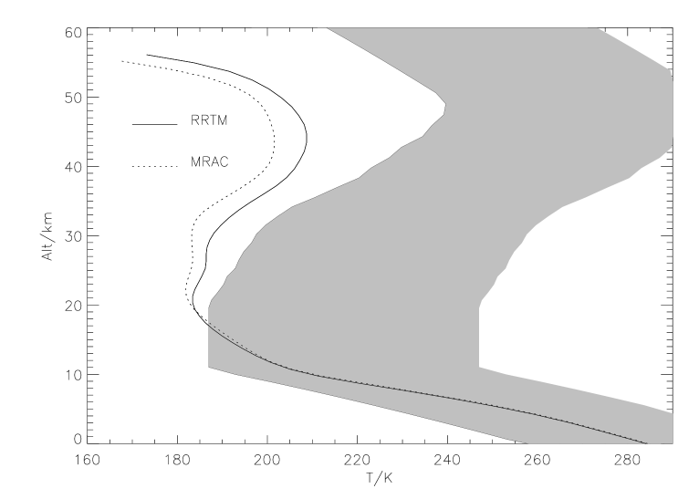
Figure 5:

Figure 6:

Figure 7:

Figure 8:

Figure 9:

Figure 10:

Figure 11:

References

- Brown et al. (2005) Brown, L. R., Benner, C., Devi, V. M., Smith, M. A. H., Toth, R. A., 2005. Line mixing in self- and foreign-broadened water vapor at 6 m. Journal of Molecular Structure 742, 111 122.
- Caldeira and Kasting (1992) Caldeira, K., Kasting, J. F., Dec. 1992. The life span of the biosphere revisited. Nature 360, 721–723.
- Cess (1976) Cess, R. D., 1976. Climatic change: An appraisal of atmospheric feedback mechanisms employing zonal climatology. J. Atmospheric Sciences 33, 1831–1843.
- Colaprete and Toon (2003) Colaprete, A., Toon, O. B., Apr. 2003. Carbon dioxide clouds in an early dense Martian atmosphere. Journal of Geophysical Research (Planets) 108, 5025.
- Goody et al. (1989) Goody, R., West, R., Chen, L., Crisp, D., Dec. 1989. The correlated-k method for radiation calculations in nonhomogeneous atmospheres. J. Quant. Spectroscopy and Radiative Transfer 42, 539–550.
- Goody and Yung (1989) Goody, R. M., Yung, Y. L., 1989. Atmospheric radiation: Theoretical basis. 2nd ed., New York, NY: Oxford University Press.
- Gough (1981) Gough, D. O., Nov. 1981. Solar interior structure and luminosity variations. Solar Physics 74, 21–34.
- Grenfell et al. (2007a) Grenfell, J. L., Grießmeier, J.-M., Patzer, B., Rauer, H., Segura, A., Stadelmann, A., Stracke, B., Titz, R., Von Paris, P., Feb. 2007a. Biomarker Response to Galactic Cosmic Ray-Induced NOx and the Methane Greenhouse Effect in the Atmosphere of an Earth-Like Planet Orbiting an M Dwarf Star. Astrobiology 7, 208–221.
- Grenfell et al. (2007b) Grenfell, J. L., Stracke, B., von Paris, P., Patzer, B., Titz, R., Segura, A., Rauer, H., Apr. 2007b. The response of atmospheric chemistry on earthlike planets around F, G and K Stars to small variations in orbital distance. Planetary and Space Science 55, 661–671.
- Haqq-Misra et al. (2008) Haqq-Misra, J., Domagal-Goldman, S., Kasting, P., Kasting, J. F., 2008. A Revised, Hazy Methane Greenhouse for the Archaean Earth. accepted in Astrobiology.
- Hessler et al. (2004) Hessler, A., Lowe, D., Jones, R., Bird, D., Apr. 2004. A lower limit for atmospheric carbon dioxide levels 3.2 billion years ago. Nature 428, 736–738.
- Ingersoll (1969) Ingersoll, A. P., Nov. 1969. The Runaway Greenhouse: A History of Water on Venus. J. Atmospheric Sciences 26, 1191–1198.
- Jenkins (2000) Jenkins, G. S., 2000. Global climate model high-obliquity solutions to the ancient climate puzzles of the Faint-Young Sun Paradox and low-latitude Proterozoic Glaciation. J. Geophys. Res. 105, 7357–7370.
- Kasting (1987) Kasting, J. F., Feb. 1987. Theoretical constraints on oxygen and carbon dioxide concentrations in the Precambrian atmosphere. Precambrian Research 34, 205–229.
- Kasting (1988) Kasting, J. F., Jun. 1988. Runaway and moist greenhouse atmospheres and the evolution of earth and Venus. Icarus 74, 472–494.
- Kasting and Ackerman (1986) Kasting, J. F., Ackerman, T. P., Dec. 1986. Climatic consequences of very high carbon dioxide levels in the Earth’s early atmosphere. Science 234, 1383–1385.
- Kasting and Howard (2006) Kasting, J. F., Howard, M. T., 2006. Atmospheric composition and climate on the early Earth. Phil. Trans. R. Soc. B 361, 1733–1742.
- Kasting et al. (1984a) Kasting, J. F., Pollack, J. B., Ackerman, T. P., Mar. 1984a. Response of earth’s atmosphere to increases in solar flux and implications for loss of water from Venus. Icarus 57, 335–355.
- Kasting et al. (1984b) Kasting, J. F., Pollack, J. B., Crisp, D., 1984b. Effects of high CO2 levels on surface temperature and atmospheric oxidation state of the early Earth. J. Atmospheric Chemistry 1, 403–428.
- Kasting et al. (1993) Kasting, J. F., Whitmire, D. P., Reynolds, R. T., Jan. 1993. Habitable Zones around Main Sequence Stars. Icarus 101, 108–128.
- Knauth and Lowe (2003) Knauth, P., Lowe, D. R., 2003. High Archean climatic temperature inferred from oxygen isotope geochemistry of cherts in the 3.5 Ga Swaziland Supergroup, South Africa. GSA Bull. 115, 566–580.
- Lacis and Oinas (1991) Lacis, A. A., Oinas, V., May 1991. A description of the correlated-k distribution method for modelling nongray gaseous absorption, thermal emission, and multiple scattering in vertically inhomogeneous atmospheres. J. Geophys. Res. 96, 9027–9064.
- Manabe and Wetherald (1967) Manabe, S., Wetherald, R. T., May 1967. Thermal Equilibrium of the Atmosphere with a Given Distribution of Relative Humidity. J. Atmospheric Sciences 24, 241–259.
- Minton and Malhotra (2007) Minton, D. A., Malhotra, R., May 2007. Assessing the Massive Young Sun Hypothesis to Solve the Warm Young Earth Puzzle. Astrophysical Journal 660, 1700–1706.
- Mischna et al. (2000) Mischna, M. A., Kasting, J. F., Pavlov, A., Freedman, R., Jun. 2000. Influence of carbon dioxide clouds on early martian climate. Icarus 145, 546–554.
- Mlawer et al. (1997) Mlawer, E. J., Taubman, S. J., Brown, P. D., Iacono, M. J., Clough, S. A., Jul. 1997. Radiative transfer for inhomogeneous atmospheres: RRTM, a validated correlated-k model for the longwave. J. Geophys. Res. 102, 16663–16682.
- Mojzsis et al. (1996) Mojzsis, S. J., Arrhenius, G., McKeegan, K. D., Harrison, T. M., Nutman, A. P., Friend, C. R. L., Nov. 1996. Evidence for life on Earth before 3,800 million years ago. Nature 384, 55–59.
- Pavlov et al. (2001) Pavlov, A. A., Brown, L. L., Kasting, J. F., Oct. 2001. UV shielding of NH3 and O2 by organic hazes in the Archean atmosphere. J. Geophys. Res. 106, 23267–23288.
- Pavlov et al. (2003) Pavlov, A. A., Hurtgen, M. T., Kasting, J. F., Arthur, M. A., Jan. 2003. Methane-rich Proterozoic atmosphere? Geology 31, 87–90.
- Pavlov et al. (2000) Pavlov, A. A., Kasting, J. F., Brown, L. L., Rages, K. A., Freedman, R., May 2000. Greenhouse warming by CH4 in the atmosphere of early Earth. J. Geophys. Res. 105, 11981–11990.
- Robert and Chaussidon (2006) Robert, F., Chaussidon, M., Oct. 2006. A palaeotemperature curve for the Precambrian oceans based on silicon isotopes in cherts . Nature 443, 969–972.
- Rosing and Frei (2004) Rosing, M. T., Frei, R., Jan. 2004. U-rich Archaean sea-floor sediments from Greenland - indications of 3700 Ma oxygenic photosynthesis. Earth and Planetary Science Letters 217, 237–244.
- Rothman et al. (1992) Rothman, L. S., Gamache, R. R., Tipping, R. H., Rinsland, C. P., Smith, M. A. H., Benner, D. C., Devi, V. M., Flaud, J.-M., Camy-Peyret, C., Perrin, A., 1992. The HITRAN molecular data base - Editions of 1991 and 1992. J. Quant. Spectroscopy and Radiative Transfer 48, 469–507.
- Rothman et al. (1995) Rothman, L. S., Wattson, R. B., Gamache, R., Schroeder, J. W., McCann, A., Jun. 1995. HITRAN HAWKS and HITEMP: high-temperature molecular database. In: Dainty, J. C. (Ed.), Proc. SPIE Vol. 2471, p. 105-111, Atmospheric Propagation and Remote Sensing IV. Presented at the Society of Photo-Optical Instrumentation Engineers (SPIE) Conference.
- Rye et al. (1995) Rye, R., Kuo, P. H., Holland, H. D., Dec. 1995. Atmospheric carbon dioxide concentrations before 2.2 billion years ago. Nature 378, 603–605.
- Sagan and Chyba (1997) Sagan, C., Chyba, C., 1997. The early faint sun paradox: Organic shielding of ultraviolet-labile greenhouse gases. Science 276, 1217–1221.
- Sagan and Mullen (1972) Sagan, C., Mullen, G., Jul. 1972. Earth and Mars: Evolution of Atmospheres and Surface Temperatures. Science 177, 52–56.
- Schreier and Böttger (2003) Schreier, F., Böttger, U., 2003. MIRART, a line-by-line code for infrared atmospheric radiation computations including derivatives. Atmospheric and Oceanic Optics 16, 262–268.
- Segura et al. (2005) Segura, A., Kasting, J. F., Meadows, V., Cohen, M., Scalo, J., Crisp, D., Butler, R. A. H., Tinetti, G., Dec. 2005. Biosignatures from Earth-Like Planets Around M Dwarfs. Astrobiology 5, 706–725.
- Segura et al. (2003) Segura, A., Krelove, K., Kasting, J. F., Sommerlatt, D., Meadows, V., Crisp, D., Cohen, M., Mlawer, E., Dec. 2003. Ozone Concentrations and Ultraviolet Fluxes on Earth-Like Planets Around Other Stars. Astrobiology 3, 689–708.
- Shaviv (2003) Shaviv, N. J., Dec. 2003. Toward a solution to the early faint Sun paradox: A lower cosmic ray flux from a stronger solar wind. J. Geophys. Res. (Space Physics) 108, 1437.
- Shields and Kasting (2007) Shields, G. A., Kasting, J. F., 2007. Palaeoclimatology: Evidence for hot early oceans? Nature 447, E1.
- Sleep and Hessler (2006) Sleep, N. H., Hessler, A. M., Jan. 2006. Weathering of quartz as an Archean climatic indicator. Earth and Planetary Science Letters 241, 594–602.
- Toon et al. (1989) Toon, O. B., McKay, C. P., Ackerman, T. P., Santhanam, K., 1989. Rapid calculation of radiative heating rates and photodissociation rates in inhomogeneous multiple scattering atmospheres. J. Geophys. Res. 94, 16287–16301.
- Toth (2000) Toth, R., 2000. Air- and N2-Broadening Parameters of Water Vapor: 604 to 2271 cm-1. J. Molec. Spectroscopy 201, 218–243.
- Towe (1985) Towe, K., 1985. Habitability of the Early Earth - Clues from the Physiology of Nitrogen Fixation and Photosynthesis. Origins of Life 15, 235–250.
- Vardavas and Carver (1984) Vardavas, I. M., Carver, J. H., Oct. 1984. Solar and terrestrial parameterizations for radiative-convective models. Planetary and Space Science 32, 1307–1325.
- Vardavas and Carver (1985) Vardavas, I. M., Carver, J. H., Oct. 1985. Atmospheric temperature response to variations in CO2 concentration and the solar-constant. Planetary and Space Science 33, 1187–1207.
- West et al. (1990) West, R., Crisp, D., Chen, L., Mar. 1990. Mapping transformations for broadband atmospheric radiation calculations. J. Quant. Spectroscopy and Radiative Transfer 43, 191–199.
- Wiscombe and Evans (1977) Wiscombe, W. J., Evans, J., 1977. Exponential-sum fitting of radiative transmission functions. Journal of Computational Physics 24, 416–444.