LAPTH-Conf-1248/08

Yukawa corrections to Higgs production associated with two bottom quarks at the LHC

We investigate the leading one-loop Yukawa corrections to the process $pp\rightarrow b\bar{b}H$ in the Standard Model. We find that the next-to-leading order correction to the cross section is small about $-4\%$ if the Higgs mass is $120$GeV. However, the appearance of leading Landau singularity when $M_{H}\geq 2M_{W}$ can lead to a large correction at the next-to-next-to-leading order level for a Higgs mass around $160$GeV.

1 Introduction

The cross section for $b\bar{b}H$ production at the LHC is very small compared to the gluon fusion channel. However, it is important to study that because of the following reasons:

• It can provide a direct measurement of the bottom-Higgs Yukawa coupling ($\lambda_{bbH}$) which can be strongly enhanced in the MSSM.

• We can identify the final state in experiment by tagging b-jets with high $p_{T}$. This reduces greatly the QCD background.

• Theoretically, it is a $2\to 3$ process at the LHC which is a good example of one-loop multi-leg calculations. Moreover, the process $gg\to b\bar{b}H$ is, to the best of our knowledge, the most beautiful example where the leading Landau singularity (LLS) occurs in an electroweak box Feynman diagram. Considering that one rarely encounters such a singularity, studying its effect is very important.

The next-to-leading order (NLO) QCD correction to the exclusive process $pp\to b\bar{b}H$ with high $p_{T}$ bottom quarks has been calculated by two groups $\!{}^{{\bf?}}$. The QCD correction is about $-22\%$ for $M_{H}=120$GeV and $\mu=M_{Z}$ (renormalisation/factorisation scale). No leading Landau singularity occurs in any QCD one-loop diagrams.

The aim of our work is to calculate the Yukawa corrections, which are the leading electroweak corrections in this case, to the exclusive $bbH$ final state with high $p_{T}$ bottom quarks at the LHC $\!{}^{{\bf?}}$. These corrections are triggered by top-charged Goldstone loops whereby, in effect, an external $b$ quark turns into a top quark. Such type of transitions can even trigger $gg\to b\bar{b}H$ even with vanishing $\lambda_{bbH}$, in which case the process is generated solely at one-loop level.

2 Calculation and results

At the LHC, the entirely dominant contribution comes from the sub-process $gg\to b\bar{b}H$. The contribution from the light quarks in the initial state is therefore neglected in our calculation. Typical Feynman diagrams at the tree and one-loop levels are shown in Fig. 1.

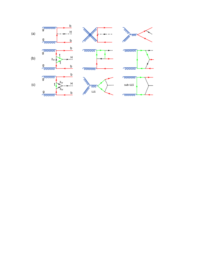
Figure 1: Typical Feynman diagrams for the process $gg\to b\bar{b}H$ at tree [class (a)] and one-loop [classes (b) and (c)] levels. Loop particles are the charged Goldstone bosons ($\chi_{W}$) and the top quark. In the class (c): the box diagram has a LLS, the pentagon diagram has the sub-leading Landau singularity which is the same as the LLS of the box diagram. The LLS occurs when $M_{H}\geq 2M_{W}$ and $\sqrt{s}\geq 2m_{t}$, i.e. all the four particles in the loop can be simultaneously on-shell.

All the relevant couplings are:

$$\lambda_{bbH} = -\frac{m_{b}}{\upsilon},\hskip 8.53581pt\lambda_{ttH}=-\frac{m_{t}}{\upsilon},$$

$$\lambda_{tb\chi} = -i\sqrt{2}\lambda_{ttH}(P_{L}-\frac{m_{b}}{m_{t}}P_{R}),\hskip 8.53581pt\lambda_{\chi^{+}\chi^{-}H}=\frac{M_{H}^{2}}{\upsilon},$$

where $\upsilon$ is the vacuum expectation value and $P_{L,R}=(1\mp\gamma_{5})/2$. The cross section as a function of $\lambda_{bbH}$ can be written in the form

$$\sigma(\lambda_{bbH}) = \sigma(\lambda_{bbH}=0)+\lambda_{bbH}^{2}\sigma^{\prime}(\lambda_{bbH}=0)+\cdots,$$

$$\lambda_{bbH}^{2}\sigma^{\prime}(\lambda_{bbH}=0) \approx \sigma_{NLO}=\sigma_{LO}[1+\delta_{NLO}(m_{t},M_{H})],$$

where $\sigma(\lambda_{bbH}=0)$ is shown in Fig. 2 (right), $\sigma_{LO}$ and $\sigma_{NLO}$ are shown in the same figure on the left.

$\sigma(\lambda_{bbH}=0)$ is generated solely at one-loop level and gets large when $M_{H}$ is close to $2M_{W}$. This is due to the leading Landau singularity related to the scalar loop integral associated to the box diagram in the class (c) of Fig. 1. This divergence, which occurs when $M_{H}\geq 2M_{W}$, is not integrable at the level of loop amplitude squared and must be regulated by introducing a width for the unstable particles in the loops. Mathematically, the width effect is to move the LLS into the complex plane so that they do not occur in the physical region. The solution is shown in Fig. 3. The important point here is that the LLS, even after being regulated, can lead to a large correction to the cross section, up to $49\%$ for $M_{H}=163$GeV, $\Gamma_{W}=2.1$GeV and $\Gamma_{t}=1.5$GeV.

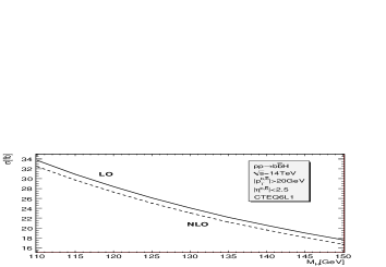
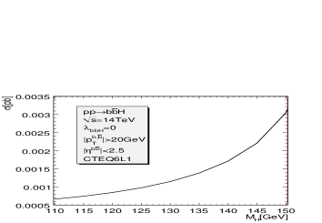
Figure 2: Left: the leading order (LO) and NLO cross sections as functions of $M_{H}$. Right: the cross section in the limit of vanishing $\lambda_{bbH}$.

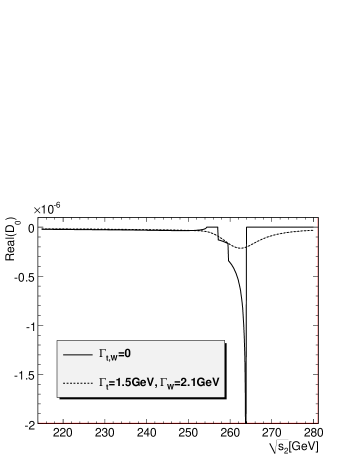
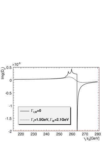
Figure 3: The real and imaginary parts of the scalar box integral associated with the LLS diagram in the class (c) of Fig. 1.

References

References

- [1] S. Dittmaier, M. Krämer and M. Spira, Phys. Rev. D70, 074010 (2004); S. Dawson, C. B. Jackson, L. Reina and D. Wackeroth, Phys. Rev. D69, 074027 (2004).
- [2] F. Boudjema and Le Duc Ninh, Phys. Rev. D77, 033003 (2008).