Models of the Cosmic Horseshoe Gravitational Lens J1004+4112

Abstract

We model the extremely massive and luminous lens galaxy in the Cosmic Horseshoe Einstein ring system J1004+4112, recently discovered in the Sloan Digital Sky Survey. We use the semi-linear method of Warren & Dye (2003), which pixelises the source surface brightness distribution, to invert the Einstein ring for sets of parameterised lens models. Here, the method is refined by exploiting Bayesian inference to optimise adaptive pixelisation of the source plane and to choose between three differently parameterised models: a singular isothermal ellipsoid, a power law model and a NFW profile. The most probable lens model is the power law with a volume mass density $\rho\propto r^{-1.96\pm 0.02}$ and an axis ratio of $\sim 0.8$. The mass within the Einstein ring (i.e., within a cylinder with projected distance of $\sim 30$ kpc from the centre of the lens galaxy) is $(5.02\pm 0.09)\times 10^{12}\,{\rm M}_{\odot}$, and the mass-to-light ratio is $\sim 30$. Even though the lens lies in a group of galaxies, the preferred value of the external shear is almost zero. This makes the Cosmic Horseshoe unique amongst large separation lenses, as almost all the deflection comes from a single, very massive galaxy with little boost from the environment.

1 Introduction

The measurement of galaxy mass distributions using strong gravitational lensing is now a well-established process, having found application to several tens of systems to date (for example, see Dye & Warren, 2007, and references therein). The main attraction of strong lensing over other methods is its insensitivity to the dynamical state of the deflecting mass.The main disadvantage is that some features of the lens mass distribution, such as the ellipticity, are much more robustly constrained by the modelling than others, such as the radial profile (Saha & Williams, 2003).

Multiple images of a background source can constrain the radial profile of the lens projected mass density only weakly (for example, see the review by Schneider, Kochanek & Wambsganss, 2006). However, some of the degeneracy is lifted by the incorporation of extra constraints from the observed velocity dispersion profile of the lens, a technique first applied by Sand, Treu & Ellis (2002) to the cluster MS 2137$-$23 and by Treu & Koopmans (2002) to the early type galaxy MG 2016+112 and subsequently to a number of systems since (Koopmans & Treu, 2003; Sand et al., 2004).

Dye & Warren (2005) showed how Einstein ring systems, i.e., strong lens systems where an extended source is imaged into a complete or near-complete ring, can constrain the mass profile of the lens more strongly than systems with multiple point-like images. This work used the semi-linear method of Warren & Dye (2003), so called because the problem of finding the best fit lens model and source surface brightness distribution is split into a linear inversion of the source for a given non-linearly parameterised lens model. The technique has been used by several other studies to date (Treu & Koopmans, 2004; Treu et al., 2006; Koopmans et al., 2006). Koopmans (2005) presented an enhanced version of the method which also reconstructs the lens gravitational potential non-parametrically. In addition, a Bayesian version of the semi-linear method was developed by Suyu et al. (2006).

In this paper, we apply the semi-linear method to reconstruct the lens mass profile and source surface brightness image of the Cosmic Horseshoe Einstein ring system J1004+4112, recently discovered in the Sloan Digital Sky Survey by Belokurov et al. (2007). This is one of the largest and most complete Einstein rings thus far discovered, with a diameter $10^{\prime\prime}$ and subtending an angle of $\sim 300^{\circ}$. The lens is an exceptionally massive Luminous Red Galaxy (LRG) with a redshift of 0.44 and a velocity dispersion of $\sim 430$ kms^-1, estimated from a mediocre signal-to-noise spectrum. The source is a star-forming galaxy of BX type, using the nomenclature of Steidel et al. (2004), with a redshift of 2.379.

Belokurov et al. (2007) already provided some simple analysis, by picking out four density knots or maxima in the ring and using techniques from the modelling of quadruply-imaged point sources to reconstruct the lensing mass (Evans & Witt, 2003). This modelling threw up a number of unresolved questions. First, there are more than four density maxima in the ring, hence Belokurov et al. (2007) provided a number of possibilities for the mass reconstruction. Their models were restricted to scale-free, isothermal-like mass profiles, though with rather general azimuthal variations. The origin of the additional density maxima in the ring was unclear – they were thought to arise from the lensing of more than one source or from higher order (sextuple) imaging. Second, although the LRG lies in a galaxy group, the group’s contribution to the lensing deflection via external shear was found to be modest. Apparently, almost all of the lensing effect is provided by the LRG itself. This is surprising because almost all the known lenses with image separations greater than $\sim 3^{\prime\prime}$ are produced by over-dense environments, with a significant lensing enhancement provided by the group or cluster. Third, although the visible light distribution of the LRG is nearly circular, the mass reconstructions were more flattened and irregular. Fourth, although Belokurov et al. (2007) provided models that matched the image location, they did not successfully reproduce the image magnifications. All this motivates a return to the Cosmic Horseshoe, but with a more sophisticated ring modelling technique.

Here, we determine the most probable mass profile for the Cosmic Horseshoe lens from three popular models. This is done by using a refinement of the semi-linear method of Warren & Dye (2003). To compare between models, we follow the technique of maximising the Bayesian evidence as derived by Suyu et al. (2006). The layout of this paper is as follows. In Section 2, we briefly describe the data. Our method of analysis is outlined in Section 3 and applied in Section 4. We summarise the findings of this work in Section 5. Throughout this paper, we assume the following cosmological parameters; ${\rm H}_{0}=70\,{\rm km\,s}^{-1}\,{\rm Mpc}^{-1}$, $\Omega_{m}=0.3$, $\Omega_{\Lambda}=0.7$.

2 Data

The Cosmic Horseshoe was discovered by Belokurov et al. (2007) by searching the Sloan Digital Sky Survey (SDSS) for luminous red galaxies with multiple, faint, blue companions. The centre of the lens galaxy lies at ($11^{h}48^{m}33.15^{s},19^{\circ}30^{\prime}3.5^{\prime\prime}$). We refer the reader to this discovery paper for full details of the data and reduction which we briefly outline here.

Follow-up imaging of the lens system was carried out in May 2007 at the 2.5m Isaac Newton Telescope (INT) in La Palma. Images were acquired in the wavebands $U$, $g$ and $i$ with the Wide Field Camera. Each image was integrated for a total of 600s and reduced with the Cambridge Astronomical Survey Unit INT pipeline (Irwin & Lewis, 2001). The data in each band are shown in the first row of Figure 1.

Long-slit spectroscopy of the lens galaxy and arc was also carried out in May 2007 at the 6m BTA telescope of the Special Astrophysical Observatory (SAO), Nizhnij Arkhyz, Russia. Absorption by Ca, H and K in the lens spectrum places the lens galaxy at a redshift of $z=0.44$. Belokurov et al. (2007) estimate a velocity dispersion of the lens of $430\pm 50$ kms^-1 by Gaussian profile fitting to the absorption lines. The slit was placed $\sim 1^{\prime\prime}$ from the centre of the lens which, given the seeing of $1.7^{\prime\prime}$ and effective radius of $\sim 2^{\prime\prime}$, means that the spectrum is dominated by flux from within the half light radius. Ly$\alpha$ emission and absorption features in the spectrum of the arc indicate that the source lies at a redshift of $z=2.38$.

To remove possible contamination of the ring by flux from the lens galaxy, we fitted an elliptical Sersic profile to the lens galaxy in each waveband. The fitted profiles were subtracted prior to our analysis. The second row in Figure 1 shows the lens removed ring image for each waveband.

Table 1 lists the $U$, $g$ and $i$ best fit parameters of the Sersic profile which has the form

$${\rm L}={\rm L}_{1/2}\exp\{-B(n)[(r/r_{0})^{1/n}-1]\}\,.$$ (1)

The parameters ${\rm L}_{1/2}$, $n$ and $r_{0}$ were allowed to vary in the fit as well as the axis ratio, $q_{s}$, (i.e., minor axis divided by major axis), orientation, $\theta_{s}$, and the centroid. We use the expression for $B(n)$ given by Ciotti & Bertin (1999). In the fitting, we convolved each trial surface brightness profile with a Gaussian point spread function (PSF) that matched the image seeing determined from stars in the field. All three fits gave acceptable $\chi^{2}$ values. Note that the ellipticity and position angle of the major axis are in good agreement with the results in Table 1 of Belokurov et al. (2007), who fitted a PSF-convolved de Vaucouleurs profile to the light distribution.

Parameter	$U$	$g$	$i$
L1/2	$1.20\pm 0.32$	$6.9\pm 0.3$	$61.2\pm 0.4$
$n$	$4.24\pm 0.4$	$4.71\pm 0.12$	$5.40\pm 0.04$
$r_{0}$ $(\prime\prime)$	$1.5\pm 2.0$	$6.1\pm 0.6$	$3.9\pm 0.1$
$\theta_{s}$ $(^{\circ})$	$85\pm 20$	$91\pm 4$	$91\pm 1$
$q_{s}$	$0.92\pm 0.12$	$0.83\pm 0.03$	$0.88\pm 0.01$

Table 1: Sersic profile parameters fit to the $U$, $g$ and $i$ band data. The normalisation L_1/2 has units of image counts matching the observed images in Figure 1. The orientation $\theta_{s}$ is in degrees counter-clockwise with respect to the positive y-axis.

3 Methodology

3.1 Bayesian Semi-linear Inversion

The original semi-linear method was derived by Warren & Dye (2003), first applied by Dye & Warren (2005) and placed within a Bayesian framework by Suyu et al. (2006). We give an outline of the method in this section but refer the reader to these publications for more comprehensive details.

The technique assumes a pixelised image and source plane. The term ‘semi-linear’ refers to the fact that the inversion problem can be divided into a set of linear parameters – the surface brightnesses of the source plane pixels – and a set of non-linear parameters that define the lens model. Generally, the source surface brightness distribution must be regularised to ensure that the linear inversion step is not mathematically ill-posed (see below). This gives rise to an extra non-linear parameter called the regularisation weight.

Warren & Dye (2003) noted that heavy regularisation biases the reconstructed source, in turn biasing the best fit lens model. Therefore, instead of applying regularisation, Dye & Warren (2005) ensured a well posed linear inversion through use of an adaptively gridded source plane. In this way, regions of the source plane that are not well constrained by the observed ring, i.e., areas of low magnification, are gridded with large pixels whilst strongly constrained areas of the source plane are more finely gridded. The degree to which source pixel sizes depend on the magnification is controlled through another non-linear parameter called the splitting factor (see below). In addition to ensuring a well posed problem, an adaptive grid has the appealing characteristic that the reconstructed source has a more uniform error map.

A more serious problem with regularisation is that it smoothes the reconstructed source, effectively increasing the number of degrees of freedom by an amount that cannot be satisfactorily quantified. This is especially problematic when comparing different lens models, as a fixed regularisation weight for one model generally does not give the same increase in number of degrees of freedom for another. Therefore, when comparing different regularised models, $\chi^{2}$ is not a useful statistic.

In the Bayesian version of the semi-linear method derived by Suyu et al. (2006), the regularisation weight is set automatically by the data. Crucially, the problem of comparing different lens models is solved by the Bayesian evidence which allows models to be objectively ranked as we describe below.

In the present work, we combine the advantages of both the Bayesian approach and an adaptive source grid. As well as allowing model ranking and regularisation, the Bayesian evidence lets the data select the optimal source pixelisation by finding the most probable splitting factor.

In the analysis outlined in the next section, it is helpful to keep the regularisation weight and splitting factor segregated from the linear source surface brightnesses and the non-linear lens model parameters. Following the terminology of Barnabè & Koopmans (2007), we will refer to these extra two non-linear parameters as ’hyperparameters’ by virtue of their indirect influence on the lens and source.

3.2 Implementation of the Inversion Method

The process of establishing the most probable lens parameterisation is split into three levels of inference. In the innermost level, the best fit source surface brightness distribution for a given set of lens model parameters and hyperparameters is determined with a linear inversion step. This proceeds as follows: A PSF-smeared image is computed for every source pixel. All images are created using unit surface brightness source pixels. The linear problem of finding the factor required to scale each image such that their co-addition best fits the observed image gives the best fit source pixel surface brightnesses, which as a vector is (Warren & Dye, 2003)

$$\mathbf{s}=({\rm\mathbf{F}}+\lambda{\rm\mathbf{H}})^{-1}\mathbf{c}\,.$$ (2)

The square matrix ${\rm\mathbf{F}}$ and the vector ${\rm\mathbf{c}}$ have the elements

$${\rm F}_{ik}=\sum_{j}f_{ij}f_{kj}/\sigma_{j}^{2}\,,\,\,\,c_{i}=\sum_{j}f_{ij}d_{j}/\sigma_{j}^{2}$$ (3)

and $\mathbf{s}$ is a vector containing the best fit source pixel surface brightnesses. Here, $d_{j}$ is the observed flux in image pixel $j$, $\sigma_{j}$ its error and $f_{ij}$ is the flux in pixel $j$ of the image of source pixel $i$ for the current lens model. The solution is regularised by the square regularisation matrix ${\rm\mathbf{H}}$, scaled by the regularisation weight $\lambda$ (see Press et al., 2001, and Warren & Dye 2003). The standard errors of the reconstructed source pixels are given by the diagonal terms of the covariance matrix $\mathbf{C}$ which is just

$$\mathbf{C}=({\rm\mathbf{F}}+\lambda{\rm\mathbf{H}})^{-1}\,.$$ (4)

In Bayesian terminology, computing the solution for $\mathbf{s}$ using equation (2) amounts to finding the most likely source surface brightness distribution by maximising the posterior probability for a given lens model and a given source pixelisation and regularisation.

In the second level of inference, the most probable set of hyperparameters for a given lens model is determined by maximising the Bayesian evidence. The evidence is a probability distribution in the lens parameters and hyperparameters that normalises the Bayesian expression for the posterior probability. It allows different models to be ranked to find the most probable model (see below). Suyu et al. (2006) derived the evidence, $\epsilon$, for this problem, which in our case can be expressed as

$$-2\,{\rm ln}\,\epsilon = \sum_{j}\left[\frac{\sum_{i}s_{i}f_{ij}-d_{j}}{\sigma_{j}}\right]^{2}+{\rm ln}\,\left[{\rm det}(\mathbf{F}+\lambda\mathbf{H})\right]$$ (5)

$$-{\rm ln}\,\left[{\rm det}(\lambda\mathbf{H})\right]+\lambda\mathbf{s}^{T}\mathbf{H\,s}+\sum_{j}{\rm ln}(2\pi\sigma_{j}^{2})\,$$

where the summations in $j$ act over all image pixels and the summation in $i$ acts over all source pixels. Here, we have assumed zero covariance between all image pixel pairs. In this expression, the first term corresponds to $\chi^{2}$ and the fourth term regularises the solution (the term denoted $\lambda G_{L}$ in the work of Warren & Dye, 2003). In this second level, equation (2) must be evaluated for every trial set of hyperparameters to allow calculation of the evidence via equation (5).

Finally, in the third and outermost level of inference, the most probable lens parameters are determined by maximising the evidence obtained from the second level. Formally, to rank models, the evidence should first be marginalised over the hyperparameters. However, Suyu et al. (2006) noted that a reasonable simplification is to approximate the distribution function of the hyperparameters as a delta function so that the maximum of the evidence obtained in the second level can be directly compared between models. We have adopted this approximation in the present study.

In practical terms, the three-level procedure can be simplified. As Barnabè & Koopmans (2007) point out, the hyperparameters that maximise the evidence in the second level of inference vary only slightly with different trial lens model parameters in the third level. This means that it is not necessary to maximise the hyperparameters with every trial lens parameter set. Instead, we alternate between varying the lens parameters whilst keeping the hyperparameters fixed and varying the hyperparameters whilst keeping the lens parameters fixed. We start this process by holding the hyperparameters (i.e., the regularisation weight and splitting factor) at a large value and varying the lens model. This reduces local maxima resulting in a smoother evidence surface so that an initial set of lens parameters lying close to the global maximum can be efficiently found (see also Warren & Dye, 2003).

We note two further practicalities. First, when computing $\chi^{2}$, i.e., the first term in equation (5), we carry out the sum over pixels contained within an annular mask that surrounds the ring. The mask is designed to include the image of the entire source plane, with minimal extraneous sky. This means that only significant image pixels are used, making the evidence more sensitive to the model parameters. Second, we use a simulated annealing downhill simplex minimisation algorithm to minimise ${\rm-ln}\,\epsilon$ given by equation (5). We find that a slow exponentially cooled temperature with a half-life of $\sim 30$ iterations works extremely well in finding the desired minimum.

3.3 Adaptive Source Plane Grid

We adaptively grid the source plane according to the prescription given in Dye & Warren (2005) and Dye et al. (2007). In this scheme, smaller pixels are concentrated in higher magnification regions where there are stronger constraints per unit area of the source plane.

The adaptive gridding algorithm starts with a regular mesh of large pixels. The average magnification $\mu_{i}$ of every source pixel $i$ is then computed. Those pixels that meet the criterion $\mu_{i}\,r_{i}\geq s$ are then split into quarters, where $r_{i}$ is the ratio of the area of pixel $i$ to the area of an image pixel and $s$ is the ‘splitting factor’. Having finished the initial loop through all pixels, the process is repeated for the sub-pixels, then for the sub-sub-pixels and so on until all pixels satisfy the splitting criterion.

The procedure is carried out every time the splitting factor is varied in the evidence maximisation. Although the adaptive grid is dependent on the lens model, we find that it does not vary significantly when varying the lens parameters. Therefore, as we discussed in the previous section, similar to the regularisation weight, we hold the splitting factor fixed whilst varying the lens parameters and vice versa, alternating until convergence is achieved. Convergence typically occurs after only a few alternate loops.

Suyu et al. (2006) advocate second order regularisation, whereby source surface brightness distributions that exhibit strongly varying gradients are penalised more heavily than those with more gradual gradient changes. Although this is simple to implement with a regular source pixel grid, it is ill-defined on an adaptive grid (one can’t define a set of co-linear pixel triplets). Instead, we apply a form of first order regularisation where strongly varying pixel-to-pixel surface brightnesses are penalised. We construct a matrix that takes the difference between a given pixel $k$ and the sum of all neighbouring pixels $l$ weighted by ${\rm w}_{kl}=(a_{l}/a_{k})\,N\exp(-y_{kl}^{2}/2\sigma^{2})$. Here, $a$ is the source pixel area, $y_{kl}$ is the separation of the centres of pixels $k$ and $l$ and $N$ is a normalisation constant set such that $\sum_{l,l\neq k}{\rm w}_{kl}=1$ and $N=1$ when $k=l$. We set $\sigma=0.2^{\prime\prime}$. The matrix $\mathbf{w}$ here relates to the regularisation matrix ${\rm\mathbf{H}}$ via ${\rm\mathbf{H}}=\mathbf{w}^{T}\mathbf{w}$. By construction, $\mathbf{H}$ is non-singular so that the third term in equation (5) is always calculable.

In Section 4, we show how each lens model prefers a different value of the splitting factor, and how this couples to the regularisation weight.

3.4 Lens models

We consider three popular mass profiles to model the distribution of the total (baryonic and dark) projected lens mass:

• Singular isothermal ellipsoid (SIE) – This model has been widely used in gravitational lensing (see e.g., Kassiola & Kovner, 1993; Schneider, Ehlers & Falco, 1992) motivated by a wealth of stellar dynamical evidence favouring the idea that galaxies are nearly isothermal. The projected surface mass density follows $\kappa=\kappa_{0}({\tilde{r}}/1{\rm kpc})^{-1}$, where ${\tilde{r}}$ is the elliptical radius defined by ${\tilde{r}}^{2}=x^{\prime 2}+q^{2}y^{\prime 2}$. The coordinates $x^{\prime}$ and $y^{\prime}$ are defined on axes aligned with the semi–major and semi–minor axes of the ellipse and $q$ is the ratio of the minor to the major axis. There are a total of five parameters for the SIE model: the normalisation $\kappa_{0}$, the orientation $\theta$, the axis ratio $q$ , and the lens centroid in the image plane, $(x_{c},y_{c})$.

• Navarro, Frenk & White (NFW) profile – This profile was introduced by Navarro, Frenk & White (1996) as a fit to dark matter halos created in cosmological N-body simulations. The lensing properties have been discussed by a number of authors (see e.g., Bartelmann, 1996; Evans & Wilkinson, 1998; Keeton, 2002). It has a projected surface mass density given by

  $$\kappa=\kappa_{0}\frac{1-F(x)}{x^{2}-1}$$ (6)

  where $x={\tilde{r}}/r_{s}$ and

  $$F(x)=\cases{{1\over\sqrt{x^{2}-1}}\,\mbox{tan}^{-1}\sqrt{x^{2}-1}&$(x>1)$\cr{1\over\sqrt{1-x^{2}}}\,\mbox{tanh}^{-1}\sqrt{1-x^{2}}&$(x<1)$\cr 1&$(x=1)$\cr}$$ (7)

  The model is described by six parameters, but we vary five in the evidence maximisation, keeping the scale radius $r_{s}$ fixed at the value of 110kpc ($\equiv 20^{\prime\prime}$ at $z=0.44$). This is in accordance with the prediction by Bullock et al. (2001) for a galaxy of similar mass and redshift to the cosmic horseshoe lens. As has been shown elsewhere (Dye et al., 2007), the lensing properties of the NFW profile depend only weakly on the value of $r_{s}$ assumed, with a 10% change in $r_{s}$ giving rise to only a $\sim 1\%$ change in the best fit model parameters. The five parameters varied in the maximisation are therefore: lens normalisation $\kappa_{0}$, orientation $\theta$, axis ratio $q$, and lens centroid in the image plane $(x_{c},y_{c})$.

• Power law (PL) – This family of models was introduced by Kassiola & Kovner (1993). The projected surface mass density is stratified on concentric ellipses following the power-law form $\kappa=\kappa_{0}\,({\tilde{r}}/{\rm 1kpc})^{1-\alpha}$. The SIE is the special case $\alpha=2$. The model has six parameters: lens normalisation $\kappa_{0}$, orientation $\theta$, axis ratio $q$, power-law slope $\alpha$ and lens centroid in the image plane $(x_{c},y_{c})$.

For each model, we maximise the evidence with and without an external shear component. The external shear adds a further two parameters to each model, a magnitude $\gamma$ and an orientation $\theta_{\gamma}$. The deflection angle required in the ray tracing has an analytic form for the SIE model, but must be numerically evaluated for the NFW and PL models, using the prescription given by Keeton (2002).

We note at this point a common misconception regarding the mass sheet degeneracy (e.g., Gorenstein, Falco & Shapiro, 1988). The degeneracy is such that image structures are invariant under the transformation $\kappa\rightarrow 1-a\,+\,a\,\kappa$ where $a$ is a constant. The degeneracy is only applicable to lens models that remain self-similar under the transformation. None of the three models applied in this paper falls into this category. For instance, applying the transformation to the power-law model does not produce a new power-law. Inverting the argument, this means that no combination of power-law parameters can give a model with a homogeneous sheet of matter and in this sense, the mass sheet degeneracy is eliminated.

4 Results

Table 2 shows the maximised parameters for the three lens models with and without external shear using the $g$ band data. The most probable model is the power law with a slope of $1.96\pm 0.02$. The evidence ranks the SIE as the next most probable model, being only 10% as probable as the power law. Finally, the NFW is strongly rejected, being ranked $>10^{-10}$ times less probable than the power law. This is perhaps not surprising given that the NFW is derived from simulations that neglect the effect of baryons.

Figure 2 shows the significance of the residuals that remain after subtracting the lensed image of the reconstructed source from the observed $g$ band ring for the SIE, PL and NFW. The NFW clearly leaves the strongest residuals as one would expect from the evidence. The difference between the PL and SIE residuals is not obvious upon visual inspection, however they differ with an RMS of $\sim 5\%$.

For the best-fitting PL model, the mass within the Einstein ring (i.e., within a cylinder with projected distance of $\sim 30$ kpc from the centre of the lens galaxy) is $(5.02\pm 0.09)\times 10^{12}\,{\rm M}_{\odot}$, as much as the entire Local Group. Using the absolute magnitude in the $r$ band of $-23.45$ computed by Belokurov et al. (2007), the mass-to-light ratio is $\sim 30$.

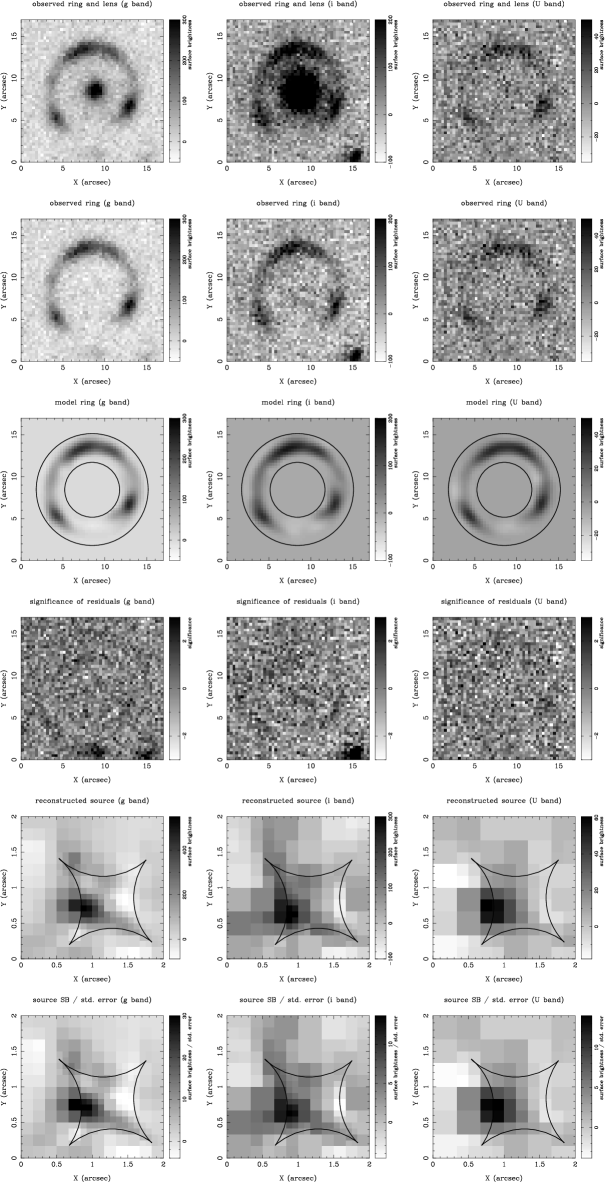
Figure 1: Image data and source reconstructions. Reading from left to right, the columns correspond to the $g$, $i$ then $U$ band data. Top row gives observed image. Second row shows the lens subtracted image. Third row is the image of the reconstructed source lensed by the most probable lens model (the ‘model image’). The annulus shows the masked area over which the $\chi^{2}$ term is evaluated when computing the evidence. Fourth row shows the significance of the residuals left after subtracting the model image from the observed ring image shown in the second row. Fifth and sixth rows respectively show the reconstructed source and the source divided by the standard errors given by the diagonal terms in the covariance matrix $\mathbf{C}$ (see Section 3.2). The northern source referred to in the text is that at ($0.7^{\prime\prime},1.4^{\prime\prime}$). Reconstructions for all three bands use the most probable PL lens model established by the $g$ band data.

Figure 3 shows the confidence regions on the hyperparameters (the regularisation weight and splitting factor). Each model has its own preferred combination of splitting factor and regularisation weight, although they are strongly degenerate. Larger splitting factors prefer smaller regularisation weights because increasing the splitting factor results in larger source plane pixels on average which effectively regularises the solution more heavily.

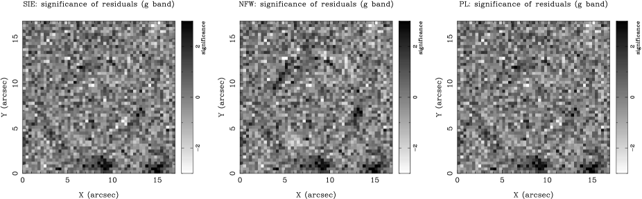
Figure 2: Significance of the residuals left after subtracting the lensed image of the reconstructed source from the observed $g$ band ring for the SIE, PL and NFW.

The source reconstructions for the PL model for each of the three wavebands are shown in Figure 1. For the $i$ and $U$ band reconstructions, we fixed the lens model parameters at their most probable values established from the $g$ band data, but varied the hyperparameters to maximise the evidence. In this way, the lens model parameters are set by the higher signal-to-noise $g$ band data, but the $i$ and $U$ band data are allowed to select the splitting factor and regularisation weight most appropriate to their information content.

Param.	SIE	NFW	PL
$\kappa_{0}$	$2.50\pm 0.03$	$0.118\pm 0.002$	$2.30\pm 0.03$
$\theta$	$46.5\pm 2.7$	$55.5\pm 3.1$	$49.2\pm 3.0$
$q$	$0.76\pm 0.03$	$0.89\pm 0.02$	$0.78\pm 0.03$
$x_{c}$	$-0.12^{\prime\prime}\pm 0.04^{\prime\prime}$	$-0.10^{\prime\prime}\pm 0.04^{\prime\prime}$	$-0.11^{\prime\prime}\pm 0.04^{\prime\prime}$
$y_{c}$	$0.05^{\prime\prime}\pm 0.03^{\prime\prime}$	$0.04^{\prime\prime}\pm 0.03^{\prime\prime}$	$0.02^{\prime\prime}\pm 0.03^{\prime\prime}$
$\alpha$	–	–	$1.96\pm 0.02$
ln $\epsilon$	$-4237.7$	$-4262.7$	$-4235.4$
Param.	SIE$+\gamma$	NFW$+\gamma$	PL$+\gamma$
$\kappa_{0}$	$2.58\pm 0.03$	$0.116\pm 0.002$	$2.37\pm 0.03$
$\theta$	$49.8\pm 2.7$	$47.9\pm 3.1$	$50.8\pm 3.1$
$q$	$0.81\pm 0.02$	$0.86\pm 0.02$	$0.83\pm 0.02$
$x_{c}$	$-0.10^{\prime\prime}\pm 0.04^{\prime\prime}$	$-0.09^{\prime\prime}\pm 0.04^{\prime\prime}$	$-0.11^{\prime\prime}\pm 0.04^{\prime\prime}$
$y_{c}$	$0.03^{\prime\prime}\pm 0.03^{\prime\prime}$	$0.04^{\prime\prime}\pm 0.03^{\prime\prime}$	$0.04^{\prime\prime}\pm 0.03^{\prime\prime}$
$\alpha$	–	–	$1.95\pm 0.02$
$\gamma$	$0.017\pm 0.005$	$0.011\pm 0.006$	$0.020\pm 0.005$
$\theta_{\gamma}$	$38.2\pm 9.4$	$46.1\pm 12.4$	$37.7\pm 8.6$
ln $\epsilon$	$-4239.0$	$-4272.0$	$-4240.2$

Table 2: Most probable parameters obtained by maximising the evidence, $\epsilon$ for each model. Parameters are: total mass normalisation $\kappa_{0}$ (in $10^{10}\,{\rm M}_{\odot}$ kpc^-2), orientation in degrees counter-clockwise with respect to the positive y-axis $\theta$, the axis ratio $q$ (minor axis divided by major axis), lens centroid in the image plane in arcseconds offset from the observed light centroid $(x_{c},y_{c})$ and the slope for the PL model $\alpha$. The top and bottom halves of the table respectively correspond to the models without and with external shear of magnitude $\gamma$ and direction $\theta_{\gamma}$.

Figure 3: 68%, 95% and 99.7% confidence regions on the splitting factor and regularisation weight, $\lambda$, for each of the three lens models using the $g$ band data. The contours are based on the Bayesian evidence and show the strong degeneracy between both parameters. Each plot is normalised to the maximum evidence for that lens model, indicated by the heavy point. The regularisation weight is scaled such that a value $\lambda=1$ weights the traces of the matrices $\mathbf{F}$ and $\mathbf{H}$ in equation (2) equally.

The velocity dispersion, $\sigma$, implied by the SIE model is given by

$$\sigma^{2}=\Sigma_{\rm CR}\,r_{E}\,G$$ (8)

where $\Sigma_{\rm CR}$ is the critical surface mass density (see Schneider, Ehlers & Falco, 1992, for example) and $r_{E}$ is the Einstein radius which relates to the SIE model parameters via

$$(r_{\rm E}/1{\rm kpc})=2\kappa_{0}\Sigma_{\rm CR}^{-1}q^{-1/2}\,.$$ (9)

This gives $r_{\rm E}=28.4$ kpc corresponding to a velocity dispersion of $496\pm 5$ kms^-1, which would make the lens one of the the most massive galaxies so far known! Nonetheless, this is consistent with the result of Gaussian fitting to absorption lines in the SAO spectrum by Belokurov et al. (2007), which yielded an estimate of 430$\pm$50 kms^-1. Although the spectrum is modest, there is little doubt that the lens is an extreme object – colour and luminosity correlate with velocity dispersion and mass, and the lens is in the brightest and reddest bins for LRGs. We emphasise that the modelling both in this paper and in Belokurov et al. (2007) does not explicitly include a velocity dispersion constraint. Hence, it is reassuring that both investigations have come to similar conclusions as regards the velocity dispersion of the lensing galaxy. Furthermore, the consistency between the two measurements implies that the stellar orbits in the LRG are nearly isotropic.

The results listed in Table 2 show that the presence of external shear is very minor. Furthermore, the evidence ranks all models incorporating shear with a lower probability than their non-sheared equivalent models. The sheared models are penalised by introducing an extra two parameters that do not bring about a significant improvement in the fit to the data.

At first, this seems surprising, as the lens is located within a group or loose cluster. With such an enormous image separation ($10^{\prime\prime}$) required, it is natural to expect a significant contribution from the environment. Even so, there is another telling indication that the environment plays only a minor role in the lensing. It was already established by Kochanek, Keeton & McLeod (2001) that the ellipticity of an Einstein ring is proportional to the external shear. The Cosmic Horseshoe ring is very nearly a perfect circle. This suggests that any perturbation from the cluster is minimal, as the mismatch between the orientation of the cluster and the lensing galaxy would generate shear and hence ellipticity in the ring. The same point is made in Saha & Williams (2003) – a narrow spread in images’ galactocentric distances indicates a small or zero external shear and moderate galaxy ellipticity. We conclude that almost all the deflection is indeed provided by one very massive galaxy, with the group environment playing a very minor role.

One curiosity is that, for the best-fitting SIE and PL models, the axis ratio of the baryonic and dark matter in Table 2 is smaller than the axis ratio of the light distribution in Table 1. There seem to be two possible resolutions of this difficulty. First, there is a well-known degeneracy between flattening and external shear. In fact, the very minor contribution from external shear, as in the models in the lower panel of Table 2, is already enough to restore the axis ratios to good agreement. Second, it is quite likely that the ellipticity of the LRG varies with radius. Although much deeper imaging is required to confirm this suggestion, there are nonetheless many local examples of giant ellipticals whose central regions are rather round, but whose outer parts are much more elongated. A good example is the nominally E0 galaxy M87, for which the ellipticity rises to 0.4 in the outer regions (Weil, Bland-Hawthorn & Malin, 1997). If a similar situation applies to the Cosmic Horseshoe lens galaxy, then the photometry of the inner parts may not be a good guide to the true shape. This may also provide an explanation as to why the position angle of the major axis of the best fit light profile is different from the angle preferred by lens models.

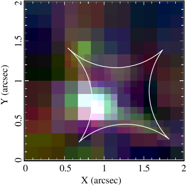
Figure 4: Colour composite of the reconstructed source. The red, green and blue channels in this image are formed respectively from the $i$, $g$ and $U$ band reconstructed sources plotted in the fifth row of Figure 1.

Finally, we note from the source reconstructions using the $g$ and $i$ band data in the bottom-most panels of Figure 1 that there is evidence for two peaks. However, the secondary northern source does not appear to be visible in the reconstruction from the noisier $U$ band data. This manifests itself in the colour composite source shown in Figure 4. The red, green and blue channels of this plot are respectively the $U$, $g$ and $i$ source surface brightness maps plotted in the fifth row of Figure 1. The northern source has a yellowish-green colour owing to the lack of $U$ band flux. Unfortunately, it is impossible to say whether this is an intrinsic colour variation or due to the lower sensitivity of the $U$ band data. Similarly, the differing source resolutions between bands prevents a clear interpretation of the colour of visible structures.

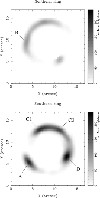
Figure 5: Images of the northern (top) and southern (bottom) reconstructed $g$ band source. The northern ring is formed by imaging all pixels northwards of the line $y=1.2^{\prime\prime}$ in the reconstructed $g$ band source shown in Figure 1 and the southern ring from all pixels to the south of this line. The ring maxima A to D follow the labelling of Belokurov et al. (2007).

The two peaks in the reconstructed source may be evidence for substructure or may indicate two sources at different redshifts. Figure 5 shows the contributions to the ring of the Cosmic Horseshoe made by each source. (Belokurov et al., 2007) already noted that there were five knots or maxima in the flux density along the ring, which they labelled A, B, C₁, $C_{2}$ and D. The southern source is mainly responsible for A, C₁, C₂ and D, whilst the effect of the northern source is to provide the additional maximum at B. As the maximum at B is barely discernible in the $U$ band image, it is no surprise that the reconstructed source in $U$ does not show any bimodality.

5 Summary

This paper has provided the first models of the Einstein ring in the newly discovered Cosmic Horseshoe gravitational lens. The semi-linear method of Warren & Dye (2003), in which the source distribution is pixelised, remains the technique of choice. For a given parametric model of the lens, the inversion of the source is linear. Here, we have exploited the refinement of adaptive gridding introduced by Dye & Warren (2005) and used the Bayesian evidence formulation of Suyu et al. (2006) to discriminate between different parametric models on an equal basis.

The lens in the Cosmic Horseshoe is a luminous red galaxy (LRG) lying in a group or loose cluster. Three different mass distributions were used to model the total luminous and dark matter in the lens – namely, an isothermal ellipsoid, a Navarro-Frenk-White profile and a power-law ellipsoid. The effects of the cluster were represented by external shear. At least as judged by Bayesian evidence, a power-law ellipsoid without shear provides the best fit. Specifically, the mass density falls off like $\rho\propto{\tilde{r}}^{-1.96\pm 0.02}$, where ${\tilde{r}}$ defines similar concentric ellipses with axis ratio $q\sim 0.8$.

Remarkably, the contribution of the group to the lensing deflection is minimal, despite the huge image separation ($10^{\prime\prime}$) in the Cosmic Horseshoe. This result is consistent with the almost circular nature of the Einstein ring. However, it means that almost all the lensing effect is produced by an enormous LRG – the velocity dispersion estimated from the modelling is $\sim 500$ kms^-1. This mildly exceeds the velocity dispersion of 430$\pm$50 kms^-1 already estimated from a low signal-to-noise spectrum by Belokurov et al. (2007). The lens galaxy appears to be the most massive LRG ever detected. The source reconstructions using the $g$ and the $i$ band data is double-peaked, although that built from the noisier $U$ band data is not. Although the nature of the double-peak remains unclear, this result is consistent with the pattern of density maxima seen along the ring.

Large separation lenses are now being routinely discovered by searches through data from the Sloan Digital Sky Survey. These probe a very different regime to the smaller separation lenses. Tools such as the ring inversion algorithm employed here can play a substantial role in understanding the distribution of matter to large radii in very massive galaxies.

References

- Barnabè & Koopmans (2007) Barnabè, M. & Koopmans, L. V. E., 2007, ApJ submitted, astro-ph/0701372
- Bartelmann (1996) Bartelmann M., 1996, AA, 313, 697
- Belokurov et al. (2007) Belokurov, V., et al., 2007, ApJ, 671, 9
- Bullock et al. (2001) Bullock, J. S., Kollat, T. S., Sigad, Y., Somerville, R. S., Kravtsov, A. V., Klypin, A. A., Primack, J. R., Deckel, A., 2001, MNRAS, 321, 598
- Ciotti & Bertin (1999) Ciotti, L. & Bertin, G., 1999, A&A, 352, 447
- Dye & Warren (2005) Dye, S. & Warren, S. J., 2005, ApJ, 623, 31
- Dye et al. (2007) Dye, S., Smail, I., Swinbank, A. M., Ebeling, H., Edge, A. C., 2007, MNRAS, 379, 308
- Dye & Warren (2007) Dye, S. & Warren, S. J., 2007, IAUS, 244, 33
- Evans & Wilkinson (1998) Evans, N. W., & Wilkinson M. I. 1998, MNRAS, 296, 800
- Evans & Witt (2003) Evans, N. W., & Witt, H. J. 2003, MNRAS, 345, 1351
- Gorenstein, Falco & Shapiro (1988) Gorenstein, M. V., Falco, E. E. & Shapiro, I. I., 1988, ApJ, 327, 693
- Irwin & Lewis (2001) Irwin, M. J. & Lewis, J. R., 2001, New Ast Rev, 45, 105
- Kassiola & Kovner (1993) Kassiola A., Kovner I., 1993, ApJ, 417, 450
- Keeton (2002) Keeton, C. R., 2002, astro-ph/0102341
- Kochanek, Keeton & McLeod (2001) Kochanek, C.S, Keeton, C., & McLeod, B.A., 2001, ApJ, 547, 50
- Koopmans & Treu (2003) Koopmans, L. V. E. & Treu, T., 2003, ApJ, 583, 606
- Koopmans (2005) Koopmans, L. V. E., 2005, MNRAS, 363, 1136
- Koopmans et al. (2006) Koopmans, L. V. E., Treu, T., Bolton, A. S., Burles, S., Moustakas, L. A., 2006, ApJ, 640, 662
- Navarro, Frenk & White (1996) Navarro, J. F., Frenk, C. S. & White S. D. M., 1996, ApJ, 462, 563
- Press et al. (2001) Press, W. H., Teukolsky, S. A., Vetterling, W. T., Flannery, B. P., 2001, ’Numerical Recipes in Fortran 77, 2nd Edition’, Cambridge University Press
- Saha & Williams (2003) Saha, P., Williams, L.L.R., 2003, AJ, 125, 2769
- Sand et al. (2004) Sand, D. J., Treu, T., Smith, G. P., Ellis, R. S., 2004, ApJ, 604, 88
- Sand, Treu & Ellis (2002) Sand, D. J., Treu, T., & Ellis, R. S., 2002, ApJ, 574, L129
- Schneider, Ehlers & Falco (1992) Schneider P., Ehlers J., Falco E.E., 1992, Gravitational Lenses (Springer-Verlag, New York)
- Schneider, Kochanek & Wambsganss (2006) Schneider, P., Kochanek, C. S. & Wambsganss, J., 2004, Part 2 of Gravitational Lensing: Strong, Weak & Micro, Proceedings of the 33rd Saas-Fee Advanced Course, (eds. G. Meylan, P. Jetzer & P. North)
- Steidel et al. (2004) Steidel, C. C., Shapley, A. E., Pettini, M., Adelberger, K. L., Erb, D. K., Reddy, N. A., & Hunt, M. P. 2004, ApJ, 604, 534
- Suyu et al. (2006) Suyu, S. H., Marshall, P. J., Hobson, M. P., Blandford, R. D., 2006, MNRAS, 371, 983
- Treu & Koopmans (2002) Treu, T. & Koopmans, L. V. E., 2002, ApJ, 575, 87
- Treu & Koopmans (2004) Treu, T. & Koopmans, L. V. E., 2004, ApJ, 611, 739
- Treu et al. (2006) Treu, T., Koopmans, L.V.E., Bolton, A. S., Burles, S., Moustakas, L. A., 2006, ApJ, 640, 662
- Warren & Dye (2003) Warren, S. J. & Dye, S., 2003, ApJ, 590, 673
- Weil, Bland-Hawthorn & Malin (1997) Weil, M. L. Bland-Hawthorn, J., & Malin D. F., 1997, ApJ, 490, 664 ,