Neutralinos and charginos in supersymmetric economical 3-3-1 model

Abstract:

Fermion superpartners - neutralinos and charginos in the supersymmetric economical 3-3-1 model are studied. By imposition $R$ parity, their masses and eigenstates are derived. Assuming that Bino-like is dark matter, its mass density is calculated. The cosmological dark matter density gives a bound on mass of LSP neutralino in the range of 20 $\div$ 100 GeV, while the bound on mass of the lightest slepton is in the range of 60 $\div$ 130 GeV

1 Introduction

The Standard Model (SM) of high energy physics provides a remarkable successful description of presently known phenomena. In spite of these successes, it fails to explain several fundamental issues like generation number puzzle, neutrino masses and oscillations, the origin of charge quantization, CP violation, etc.

One of the simplest solutions to these problems is to enhance the SM symmetry $\mathrm{SU}(3)_{C}\otimes\mathrm{SU}(2)_{L}\otimes\mathrm{U}(1)_{Y}$ to $\mathrm{SU}(3)_{C}\otimes\mathrm{SU}(3)_{L}\otimes\mathrm{U}(1)_{X}$ (called 3-3-1 for short) [1, 2, 3] gauge group. One of the main motivations to study this kind of models is an explanation in part of the generation number puzzle. In the 3-3-1 models, each generation is not anomaly free; and the model becomes anomaly free if one of quark families behaves differently from other two. Consequently, the number of generations is multiple of the color number. Combining with the QCD asymptotic freedom, the generation number has to be three. For the neutrino masses and oscillations, the electric charge quantization and CP violation issues in the 3-3-1 models, the interested readers can find in Refs. [4], [5] and [6], respectively.

In one of the 3-3-1 models, the right-handed neutrinos are in bottom of the lepton triplets [3] and three Higgs triplets are required. It is worth noting that, there are two Higgs triplets with neutral components in the top and bottom. In the earlier version, these triplets can have vacuum expectation value (VEV) either on the top or in the bottom, but not in both. Assuming that all neutral components in the triplet can have VEVs, we are able to reduce number of triplets in the model to be two  [7, 8] (for a review, see  [9]). Such a scalar sector is minimal, therefore it has been called the economical 3-3-1 model [10]. In a series of papers, we have developed and proved that this non-supersymmetric version is consistent, realistic and very rich in physics [8, 10, 11, 12].

In the other hands, due to the “no-go” theorem of Coleman-Mandula [13], the internal $G$ and external $P$ spacetime symmetries can only be trivially unified. In addition, the mere fact that the ratio $M_{P}/M_{W}$ is so huge is already a powerful clue to the character of physics beyond the SM, because of the infamous hierarchy problem. In the framework of new symmetry called a supersymmetry [14, 15], the above mentioned problems can be solved. One of the intriguing features of supersymmetric theories is that the Higgs spectrum (unfortunately, the only part of the SM is still not discovered) is quite constrained.

It is known that the economical (non-supersymmetric) 3-3-1 model does not furnish any candidate for self-interaction dark matter [16] with the condition given by Spergel and Steinhardt [17]. With a larger content of the scalar sector, the supersymmetric version is expected to have a candidate for the self-interaction dark matter. An supersymmetric version of the minimal version (without extra lepton) has been constructed in Ref. [18] and its scalar sector was studied in Ref. [19]. Lepton masses in framework of the above mentioned model was presented in Ref. [20], while potential discovery of supersymmetric particles was studied in [21]. In Ref. [22], the $R$ - parity violating interaction was applied for instability of the proton.

The supersymmetric version of the 3-3-1 model with right-handed neutrinos [3] has already been constructed in Ref. [23]. The scalar sector was considered in Ref. [24] and neutrino mass was studied in Ref. [25]. Note that there is three-family versions in which lepton families are treated differently  [26] and their supersymmetric versions are presented in Ref. [27]. It is worth mentioning that in the previous papers on supersymmetric version of the 3-3-1 models, the main attention was given to the gauge boson, lepton mass and Higgs sectors. An supersymmetric version of the economical 3-3-1 model has been constructed in Ref. [28]. Some interesting features such as Higgs bosons with masses equal to that of the gauge bosons – the $W$ and the bileptons $X$ and $Y$, have been pointed out in Ref. [29]. Sfermions have been considered in Ref. [30].

In a supersymmetric extension of the (beyond) SM, each of the known fundamental particles must be in either a chiral or gauge supermultiplet and have a superpartner with spin differing by 1/2 unit. Both gauge and scalar bosons have spin-$\frac{1}{2}$ superpartners with the electric charges equal to that of their originals: called neutralinos without electric charge and charginos if carrying the latter one. In the Minimal Supersymmetric Standard Model (MSSM), in some scenario, the neutralino can be the lightest and plays a role of dark matter. In this paper, we will focus an attention to neutralinos and charginos in the supersymmetric economical 3-3-1 model.

This article is organized as follows. In Sec. 2 we present fermion and scalar content in the supersymmetric economical 3-3-1 model. The necessary parts of Lagrangian is also given. In Section 3, we deal with neutralinos sector. To find eigenstates and their masses, we have to adopt some assumptions. Section 4 is devoted for charginos. In Section 5 we present analysis of relic neutralino dark matter mass density and the limit on its mass. Finally, we summarize our results and make conclusions in the last section - Sec. 6.

2 A review of the model

In this section we first recapitulate the basic elements of the supersymmetric economical 3-3-1 model [28]. $R-parity$ and some constraints on the couplings are also presented.

2.1 Particle content

The superfield content in this paper is defined in a standard way as follows

$$\widehat{F}=(\widetilde{F},F),\hskip 14.22636pt\widehat{S}=(S,\widetilde{S}),\hskip 14.22636pt\widehat{V}=(\lambda,V),$$ (1)

where the components $F$, $S$ and $V$ stand for the fermion, scalar and vector fields while their superpartners are denoted as $\widetilde{F}$, $\widetilde{S}$ and $\lambda$, respectively [14, 23].

The superfield content in the considering model with an anomaly-free fermionic content transforms under the 3-3-1 gauge group as

$$\widehat{L}_{aL}=\left(\widehat{\nu}_{a},\widehat{l}_{a},\widehat{\nu}^{c}_{a}\right)^{T}_{L}\sim(1,3,-1/3),\hskip 14.22636pt\widehat{l}^{c}_{aL}\sim(1,1,1),$$

$$\widehat{Q}_{1L}=\left(\widehat{u}_{1},\ \widehat{d}_{1},\ \widehat{u}^{\prime}\right)^{T}_{L}\sim(3,3,1/3),$$

$$\widehat{u}^{c}_{1L},\ \widehat{u}^{\prime c}_{L}\sim(3^{*},1,-2/3),\hskip 14.22636pt\widehat{d}^{c}_{1L}\sim(3^{*},1,1/3),$$

$$\begin{array}[]{ccc}\widehat{Q}_{\alpha L}=\left(\widehat{d}_{\alpha},-\widehat{u}_{\alpha},\widehat{d^{\prime}}_{\alpha}\right)^{T}_{L}\sim(3,3^{*},0),\hskip 14.22636pt\alpha=2,3,\end{array}$$

$$\widehat{u}^{c}_{\alpha L}\sim\left(3^{*},1,-2/3\right),\hskip 14.22636pt\widehat{d}^{c}_{\alpha L},\ \widehat{d}^{\prime c}_{\alpha L}\sim\left(3^{*},1,1/3\right),$$

where the values in the parentheses denote quantum numbers based on $\left(\mbox{SU}(3)_{C}\right.$, $\mbox{SU}(3)_{L}$, $\left.\mbox{U}(1)_{X}\right)$ symmetry. $\widehat{\nu}^{c}_{L}=(\widehat{\nu}_{R})^{c}$ and $a=1,2,3$ is a generation index. The primes superscript on usual quark types ($u^{\prime}$ with the electric charge $q_{u^{\prime}}=2/3$ and $d^{\prime}$ with $q_{d^{\prime}}=-1/3$) indicate that those quarks are exotic ones.

The two superfields $\widehat{\chi}$ and $\widehat{\rho}$ are at least introduced to span the scalar sector of the economical 3-3-1 model [10]:

$$\widehat{\chi} = \left(\widehat{\chi}^{0}_{1},\widehat{\chi}^{-},\widehat{\chi}^{0}_{2}\right)^{T}\sim(1,3,-1/3),$$

$$\widehat{\rho} = \left(\widehat{\rho}^{+}_{1},\widehat{\rho}^{0},\widehat{\rho}^{+}_{2}\right)^{T}\sim(1,3,2/3).$$

To cancel the chiral anomalies of higgsino sector, the two extra superfields $\widehat{\chi}^{\prime}$ and $\widehat{\rho}^{\prime}$ must be added as follows

$$\widehat{\chi}^{\prime} = \left(\widehat{\chi}^{\prime 0}_{1},\widehat{\chi}^{\prime+},\widehat{\chi}^{\prime 0}_{2}\right)^{T}\sim(1,3^{*},1/3),$$

$$\widehat{\rho}^{\prime} = \left(\widehat{\rho}^{\prime-}_{1},\widehat{\rho}^{\prime 0},\widehat{\rho}^{\prime-}_{2}\right)^{T}\sim(1,3^{*},-2/3).$$

In this model, the $\mathrm{SU}(3)_{L}\otimes\mathrm{U}(1)_{X}$ gauge group is broken via two steps:

$$\mathrm{SU}(3)_{L}\otimes\mathrm{U}(1)_{X}\stackrel{{\scriptstyle w,w^{\prime}}}{{\longrightarrow}}\ \mathrm{SU}(2)_{L}\otimes\mathrm{U}(1)_{Y}\stackrel{{\scriptstyle v,v^{\prime},u,u^{\prime}}}{{\longrightarrow}}\mathrm{U}(1)_{Q},$$ (2)

where the VEVs are defined by

$$\sqrt{2}\langle\chi\rangle^{T} = \left(u,0,w\right),\hskip 14.22636pt\sqrt{2}\langle\chi^{\prime}\rangle^{T}=\left(u^{\prime},0,w^{\prime}\right),$$ (3)

$$\sqrt{2}\langle\rho\rangle^{T} = \left(0,v,0\right),\hskip 14.22636pt\sqrt{2}\langle\rho^{\prime}\rangle^{T}=\left(0,v^{\prime},0\right).$$

The VEVs $w$ and $w^{\prime}$ are responsible for the first step of the symmetry breaking while $u,\ u^{\prime}$ and $v,\ v^{\prime}$ are for the second one. Therefore, they have to satisfy the constraints:

$$u,\ u^{\prime},\ v,\ v^{\prime}\ll w,\ w^{\prime}.$$ (4)

It is emphasized that the VEV structure in (3) is not only the key to reduce Higgs sector but also the reason for complicated mixing among gauge, Higgs bosons, etc. As it will be shown in the following, the mentioned VEV structure causes flavour violation in the $D$-term contributions.

The vector superfields $\widehat{V}_{c}$, $\widehat{V}$ and $\widehat{V}^{\prime}$ containing the usual gauge bosons are, respectively, associated with the $\mathrm{SU}(3)_{C}$, $\mathrm{SU}(3)_{L}$ and $\mathrm{U}(1)_{X}$ group factors. The colour and flavour vector superfields have expansions in the Gell-Mann matrix bases $T^{a}=\lambda^{a}/2$ $(a=1,2,...,8)$ as follows

$$\widehat{V}_{c} = \frac{1}{2}\lambda^{a}\widehat{V}_{ca},\hskip 14.22636pt\widehat{\overline{V}}_{c}=-\frac{1}{2}\lambda^{a*}\widehat{V}_{ca};\hskip 14.22636pt\widehat{V}=\frac{1}{2}\lambda^{a}\widehat{V}_{a},\hskip 14.22636pt\widehat{\overline{V}}=-\frac{1}{2}\lambda^{a*}\widehat{V}_{a},$$

where an overbar ^- indicates complex conjugation. For the vector superfield associated with $\mathrm{U}(1)_{X}$, we normalize as follows

$$X\hat{V}^{\prime}=(XT^{9})\hat{B},\hskip 14.22636ptT^{9}\equiv\frac{1}{\sqrt{6}}\mathrm{diag}(1,1,1).$$

The gluons are denoted by $g^{a}$ and their respective gluino partners by $\lambda^{a}_{c}$, with $a=1,\ldots,8$. In the electroweak sector, $V^{a}$ and $B$ stand for the $\mathrm{SU}(3)_{L}$ and $\mathrm{U}(1)_{X}$ gauge bosons with their gaugino partners $\lambda^{a}_{V}$ and $\lambda_{B}$, respectively.

With the superfields as given, the full Lagrangian is defined by $\mathcal{L}_{susy}+\mathcal{L}_{soft}$, where the first term is supersymmetric part, whereas the last term breaks explicitly the supersymmetry [28]. The interested reader can find more details on this Lagrangian in the above mentioned article. In the following, only terms relevant to our calculations are displayed.

2.2 $R$-parity

For the further analysis, it is convenience to introduce $R$-parity in the model. Following Ref. [25], $R$-parity can be expressed as follows

$$R-parity=(-1)^{2S}(-1)^{3({\mathcal{B}}+{\mathcal{L}})}$$ (5)

where invariant charges ${\mathcal{L}}$ and ${\mathcal{B}}$ (for details, see Ref. [31]) are given by [30]

$$\begin{array}[]{|c|c|c|c|c|}\hline\cr Triplet&L&Q_{1}&\chi&\rho\\ \hline\cr{\mathcal{B}}\,\ charge&0&\frac{1}{3}&0&0\\ \hline\cr{\mathcal{L}}\,\ charge&\frac{1}{3}&-\frac{2}{3}&\frac{4}{3}&-\frac{2}{3}\\ \hline\cr\end{array}$$ (6)

$$\begin{array}[]{|c|c|c|c|}\hline\cr Anti-Triplet&Q_{\alpha}&\chi^{\prime}&\rho^{\prime}\\ \hline\cr{\mathcal{B}}\,\ charge&\frac{1}{3}&0&0\\ \hline\cr{\mathcal{L}}\,\ charge&\frac{2}{3}&-\frac{4}{3}&\frac{2}{3}\\ \hline\cr\end{array}$$ (7)

$$\begin{array}[]{|c|c|c|c|c|c|}\hline\cr Singlet&l^{c}&u^{c}&d^{c}&u^{\prime c}&d^{\prime c}\\ \hline\cr{\mathcal{B}}\,\ charge&0&-\frac{1}{3}&-\frac{1}{3}&-\frac{1}{3}&-\frac{1}{3}\\ \hline\cr{\mathcal{L}}\,\ charge&-1&0&0&2&-2\\ \hline\cr\end{array}$$ (8)

3 The neutralinos sector

The higginos and electroweak gauginos mix each with other due to effects of the electroweak symmetry breaking. The neutral higginos and gauginos combine to make the mass eigenvectors called neutralinos. In this section, the mass spectrum and mixing of the neutralinos is considered.

The gauginos mass terms come directly from the soft term given by

$$\mathcal{L}_{Soft}=\sum_{b=1}^{8}M_{b}\widetilde{\mathcal{W}}^{b}\widetilde{\mathcal{W}}^{b}+M_{\widetilde{\mathcal{B}}}\widetilde{\mathcal{B}}\widetilde{\mathcal{B}}.$$ (9)

Because of the R-parity conservation, the higginos mixing terms come from the $\mu-$term determined as

$$\mathcal{L}_{\mu-term}=\mu_{\chi}\widehat{\chi}\widehat{\chi}^{\prime}+\mu_{\rho}\widehat{\rho}\widehat{\rho}^{\prime}.$$ (10)

Finally, the mixing terms between higginos and gauginos are a result of Higgs-higginos-gauginos couplings

$$\mathcal{L}=-\sqrt{2}g\left(\phi^{*}T^{a}\psi\right)\lambda^{a}-\sqrt{2}g\lambda^{+a}\left(\psi^{+}T^{a}\phi\right).$$ (11)

Expanding Eqs (9), (10) and (11), we obtain the neutralino mass matrix in the gauge-eigenatates basis $\psi^{o}=\left(\widetilde{\chi^{o}_{1}},\widetilde{\chi^{o\prime}_{1}},\widetilde{\chi^{o}_{2}},\widetilde{\chi^{o\prime}_{2}},\widetilde{\rho^{o}_{1}},\widetilde{\rho^{o\prime}_{1}},\widetilde{\mathcal{B}},\widetilde{\mathcal{W}_{3}},\widetilde{\mathcal{W}_{8}},\widetilde{\mathcal{X}},\widetilde{\mathcal{X}^{*}}\right)$, which is given in the Lagrangian form

$$\mathcal{L}=\left(\widetilde{\psi^{o}}\right)^{T}M_{\widetilde{N}}\widetilde{\psi^{o}}$$ (12)

with the following notations

$$\widetilde{\mathcal{X}}=\frac{\widetilde{\mathcal{W}}_{4}+i\widetilde{\mathcal{W}}_{5}}{2},\widetilde{\mathcal{X^{*}}}=\frac{\widetilde{\mathcal{W}}_{4}-i\widetilde{\mathcal{W}}_{5}}{2}$$ (13)

and

$$M_{\widetilde{N}}=\left(\begin{array}[]{ccccccccccc}0&-\mu_{\chi}&0&0&0&0&-\frac{g^{\prime}u}{3\sqrt{6}}&\frac{gu}{2}&\frac{gu}{2\sqrt{3}}&\frac{gw}{\sqrt{2}}&0\\ -\mu_{\chi}&0&0&0&0&0&\frac{g^{\prime}u^{\prime}}{3\sqrt{6}}&\frac{gu^{\prime}}{2}&\frac{gu^{\prime}}{2\sqrt{3}}&\frac{gw^{\prime}}{\sqrt{2}}&0\\ 0&0&0&&-\mu_{\chi}&0&-\frac{g^{\prime}w}{3\sqrt{6}}&0&-\frac{gw}{\sqrt{3}}&0&\frac{gu}{\sqrt{2}}\\ 0&0&-\mu_{\chi}&0&0&0&\frac{g^{\prime}w^{\prime}}{3\sqrt{6}}&0&-\frac{gw^{\prime}}{\sqrt{3}}&0&\frac{gu^{\prime}}{\sqrt{2}}\\ 0&0&0&0&0&-\mu_{\rho}&\frac{2g^{\prime}v}{3\sqrt{6}}&-\frac{gv}{2}&\frac{gv}{2\sqrt{3}}&0&0\\ 0&0&0&0&-\mu_{\rho}&0&-\frac{2g^{\prime}v^{\prime}}{3\sqrt{6}}&-\frac{gv^{\prime}}{2}&\frac{gv^{\prime}}{2\sqrt{3}}&0&0\\ -\frac{g^{\prime}u}{3\sqrt{6}}&\frac{g^{\prime}u^{\prime}}{3\sqrt{6}}&-\frac{g^{\prime}w}{3\sqrt{6}}&\frac{g^{\prime}w^{\prime}}{3\sqrt{6}}&\frac{2g^{\prime}v}{3\sqrt{6}}&-\frac{2g^{\prime}v^{\prime}}{3\sqrt{6}}&\mathcal{M_{B}}&0&0&0&0\\ \frac{gu}{2}&\frac{gu^{\prime}}{2}&0&0&-\frac{gv}{2}&-\frac{gv^{\prime}}{2}&0&\mathcal{M}_{3}&0&0&0\\ \frac{gu}{2\sqrt{3}}&\frac{gu^{\prime}}{2\sqrt{3}}&-\frac{gw}{\sqrt{3}}&-\frac{gw^{\prime}}{\sqrt{3}}&\frac{gv}{2\sqrt{3}}&\frac{gv^{\prime}}{2\sqrt{3}}&0&0&\mathcal{M}_{8}&0&0\\ \frac{gw}{2}&\frac{gw^{\prime}}{2}&0&0&0&0&0&0&0&\mathcal{M}_{45}&0\\ 0&0&\frac{gu}{2}&\frac{gu^{\prime}}{2}&0&0&0&0&0&0&\mathcal{M}_{45}\end{array}\right)\\$$

where $\mathcal{M}_{4}=\mathcal{M}_{5}\equiv\mathcal{M}_{45}$. The mass matrix $M_{\widetilde{N}}$ can be diagonalized by an unitary matrix $U$ to get the mass eigenstates. It means that we can find matrix $U$ satisfying:

$$UMU^{-1} = \textrm{Diag}(m_{\widetilde{N}_{1}},m_{\widetilde{N}_{2}},m_{\widetilde{N}_{3}}m_{\widetilde{N}_{4}},m_{\widetilde{N}_{5}},m_{\widetilde{N}_{6}},m_{\widetilde{N}_{7}},$$ (14)

$$m_{\widetilde{N}_{8}},m_{\widetilde{N}_{9}},m_{\widetilde{N}_{10}},m_{\widetilde{N}_{11}})$$

with real positive entries on the diagonal.

In general, the parameters $\mathcal{M}_{B},\mathcal{M}_{3},\mathcal{M}_{8},\mathcal{M}_{45},\mu_{\chi},\mu_{\rho}$ can take arbitrary complex phase. However we can choose a convention to make $\mathcal{M}_{B},\mathcal{M}_{3},\mathcal{M}_{8},\mathcal{M}_{45}$ to be all real and positive. If we choose the parameter $\mu_{\chi},\mu_{\rho}$ to be real and positive then we must pick up the $\left\langle\chi\right\rangle,\left\langle\chi^{\prime}\right\rangle,\left\langle\rho\right\rangle,\left\langle\rho^{\prime}\right\rangle$ to be real and positive too. If $\mu_{\chi}$ and $\mu_{\rho}$ are not real, then we obtain the CP violating effects in the potential. Therefore, as the same as in the MSSM  [15], it is convinience to choose the $\mu_{\chi},\mu_{\rho}$ to be real but without fixing the sign of $\mu_{\chi},\mu_{\rho}$.

Getting exact eigenvalues and eigenstates of the mixing mass matrix (3) is very difficult task. Hence, we make some assumptions which is suitable for theoretical comments; and their correctness could be tested by the future experiments.

In this paper, we assume that

$$v,v^{\prime},u,u^{\prime},w,w^{\prime}\ll\left|\mu_{\rho}-\mathcal{M}_{\mathcal{B}}\right|,\left|\mu_{\rho}-\mathcal{M}_{3}\right|,\left|\mu_{\rho}-\mathcal{M}_{8}\right|,\left|\mu_{\rho}-\mathcal{M}_{45}\right|$$ (15)

and

$$v,v^{\prime},u,u^{\prime},w,w^{\prime}\ll\left|\mu_{\chi}-\mathcal{M}_{\mathcal{B}}\right|,\left|\mu_{\chi}-\mathcal{M}_{3}\right|,\left|\mu_{\chi}-\mathcal{M}_{8}\right|,\left|\mu_{\chi}-\mathcal{M}_{45}\right|.$$ (16)

In the above limit, using a small perturbation on the neutralinos mass matrix (3), we can obtain the neutralino mass eigenstates, which are nearly a “higginos-like”, a “Bino-like”, a “zino-like”, an “extrazino-like ”, a “xino-like”, and the conjugated of the “xino-like” corresponding to

$$\widetilde{N}_{1}=\widetilde{\mathcal{B}},\widetilde{N}_{2}=\widetilde{\mathcal{W}}_{3},\widetilde{N}_{3}=\widetilde{\mathcal{W}}_{8},\widetilde{N}_{4}=\widetilde{\mathcal{X}^{*}},\widetilde{N}_{5}=\widetilde{\mathcal{X}},$$

$$\widetilde{N}_{6},\widetilde{N}_{7}=\frac{\widetilde{\rho}^{o}\pm\widetilde{\rho^{\prime o}_{1}}}{\sqrt{2}},\widetilde{N}_{8},\widetilde{N}_{9}=\frac{\widetilde{\chi^{o}}_{1}\pm\widetilde{\chi^{o\prime}_{1}}}{\sqrt{2}},\widetilde{N}_{10},\widetilde{N}_{11}=\frac{\widetilde{\chi^{o}}_{2}\pm\widetilde{\chi^{\prime o}_{2}}}{\sqrt{2}}$$ (17)

with the mass eigenvalues:

$$m_{\widetilde{N}_{1}} = \mathcal{M}_{\mathcal{B}}+\frac{g^{\prime 2}\left[\left(u+u^{\prime}\right)^{2}+\left(w+w^{\prime}\right)^{2}\right]}{108\left(\mathcal{M}_{\mathcal{B}}+\mu_{\chi}\right)}+\frac{g^{\prime 2}\left[\left(u-u^{\prime}\right)^{2}+\left(w-w^{\prime}\right)^{2}\right]}{108\left(\mathcal{M}_{\mathcal{B}}-\mu_{\chi}\right)}$$

$$+\frac{g^{\prime 2}\left(v-v^{\prime}\right)^{2}}{27\left(\mathcal{M}_{\mathcal{B}}-\mu_{\rho}\right)}+\frac{g^{\prime 2}\left(v+v^{\prime}\right)^{2}}{27\left(\mathcal{M}_{\mathcal{B}}+\mu_{\rho}\right)},$$

$$m_{\widetilde{N}_{2}} = \mathcal{M}_{3}+\frac{g^{2}\left(u-u^{\prime}\right)^{2}}{8\left(\mathcal{M}_{3}+\mu_{\chi}\right)}+\frac{g^{2}\left(u+u^{\prime}\right)^{2}}{8\left(\mathcal{M}_{3}-\mu_{\chi}\right)}$$

$$+\frac{g^{2}\left(v+v^{\prime}\right)^{2}}{8\left(\mathcal{M}_{3}-\mu_{\rho}\right)}+\frac{g^{2}\left(v-v^{\prime}\right)^{2}}{8\left(\mathcal{M}_{3}+\mu_{\rho}\right)},$$

$$m_{\widetilde{N}_{3}} = \mathcal{M}_{8}+\frac{g^{2}\left[\left(u-u^{\prime}\right)^{2}+4\left(w-w^{\prime}\right)^{2}\right]}{24\left(\mathcal{M}_{8}+\mu_{\chi}\right)}+\frac{g^{2}\left[\left(u+u^{\prime}\right)^{2}+4\left(w+w^{\prime}\right)^{2}\right]}{24\left(\mathcal{M}_{8}-\mu_{\chi}\right)}$$

$$+\frac{g^{2}\left(v-v^{\prime}\right)^{2}}{24\left(\mathcal{M}_{8}+\mu_{\rho}\right)}+\frac{g^{2}\left(v+v^{\prime}\right)^{2}}{24\left(\mathcal{M}_{8}-\mu_{\rho}\right)},$$

$$m_{\widetilde{N}_{4}} = \mathcal{M}_{45}+\frac{g^{2}\left[2\mu_{\chi}uu^{\prime}+\mathcal{M}_{45}\left(u^{2}+u^{\prime 2}\right)\right]}{2\left(\mathcal{M}_{45}^{2}-\mu_{\chi}^{2}\right)},$$

$$m_{\mathcal{\widetilde{N}}_{5}} = \mathcal{M}_{45}+\frac{g^{2}\left[2\mu_{\chi}ww^{\prime}+\mathcal{M}_{45}\left(w^{2}+w^{\prime 2}\right)\right]}{2\left(\mathcal{M}_{45}^{2}-\mu_{\chi}^{2}\right)},$$

$$m_{\widetilde{N}_{6}} = \left|\mu_{\rho}\right|+\frac{g^{2}\left(v-v^{\prime}\right)^{2}}{8\left(\mu_{\rho}-\mathcal{M}_{3}\right)}+\frac{g^{2}\left(v-v^{\prime}\right)^{2}}{24\left(\mu_{\rho}-\mathcal{M}_{8}\right)}+\frac{g^{\prime 2}\left(v+v^{\prime}\right)^{2}}{27\left(\mu_{\rho}-\mathcal{M}_{\mathcal{B}}\right)},$$

$$m_{\widetilde{N}_{7}} = \left|\mu_{\rho}\right|+\frac{g^{2}\left(v+v^{\prime}\right)^{2}}{8\left(\mu_{\rho}-\mathcal{M}_{3}\right)}+\frac{g^{2}\left(v+v^{\prime}\right)^{2}}{24\left(\mu_{\rho}-\mathcal{M}_{8}\right)}+\frac{g^{\prime 2}\left(v-v^{\prime}\right)^{2}}{27\left(\mu_{\rho}-\mathcal{M}_{\mathcal{B}}\right)},$$

$$m_{\widetilde{N}_{8}} = \left|\mu_{\chi}\right|+\frac{1}{2}\left[m_{a11}+m_{a22}-\sqrt{\left(m_{a11}-m_{a22}\right)^{2}+4m_{a12}^{2}}\right],$$

$$m_{\widetilde{N}_{9}} = \left|\mu_{\chi}\right|+\frac{1}{2}\left[m_{b11}+m_{b22}-\sqrt{\left(m_{b11}-m_{b22}\right)^{2}+4m_{b12}^{2}}\right],$$

$$m_{\widetilde{N}_{10}} = \left|\mu_{\chi}\right|+\frac{1}{2}\left[m_{a11}+m_{a22}+\sqrt{\left(m_{a11}-m_{a22}\right)^{2}+4m_{a12}^{2}}\right],$$

$$m_{\widetilde{N}_{11}} = \left|\mu_{\chi}\right|+\frac{1}{2}\left[m_{b11}+m_{b22}+\sqrt{\left(m_{b11}-m_{b22}\right)^{2}+4m_{b12}^{2}}\right]$$ (18)

where

$$m_{a11} = \frac{1}{126}\left[\frac{-2g^{\prime 2}\left(u-u^{\prime}\right)^{2}}{\mathcal{M}_{\mathcal{B}}-\mu_{\chi}}+9g^{2}\left(\frac{3}{\mu_{\chi}-\mathcal{M}_{3}}+\frac{1}{\mu_{\chi}-\mathcal{M}_{8}}\right)\left(u+u^{\prime}\right)^{2}\right]$$

$$-\frac{3g^{2}\left(w+w^{\prime}\right)^{2}}{7\left(M_{45}-\mu_{\chi}\right)},$$

$$m_{a12} = \frac{-g^{\prime 2}\left(u-u^{\prime}\right)\left(w-w^{\prime}\right)}{108\left(\mathcal{M}_{\mathcal{B}}-\mu_{\chi}\right)}+\frac{g^{2}\left(u+u^{\prime}\right)\left(w+w^{\prime}\right)}{12\left(\mathcal{M}_{8}-\mu_{\chi}\right)},$$

$$m_{a22} = -\frac{g^{2}}{12\left(\mathcal{M}_{8}-\mu_{\chi}\right)\left(\mathcal{M}_{45}-\mu_{\chi}\right)}\left\{3\mathcal{M}_{8}\left(u+u^{\prime}\right)^{2}+2\mathcal{M}_{45}\left(w+w^{\prime}\right)^{2}\right.$$

$$\left.-\mu_{\chi}\left[3\left(u+u^{\prime}\right)^{2}+\left(w+w^{\prime}\right)^{2}\right]\right\}-\frac{1}{108}\frac{g^{\prime 2}\left(w-w^{\prime}\right)^{2}}{\mathcal{M}_{\mathcal{B}}-\mu_{\chi}},$$

$$m_{b11} = -\frac{1}{108}\frac{g^{\prime 2}\left(u+u^{\prime}\right)^{2}}{\mathcal{M}_{\mathcal{B}}+\mu_{\chi}}-\frac{g^{2}\left(w-w^{\prime}\right)^{2}}{4\left(\mathcal{M}_{45}+\mu_{\chi}\right)}$$

$$-\frac{g^{2}}{26}\left(\frac{3}{\mathcal{M}_{3}+\mu_{\chi}}+\frac{1}{\mathcal{M}_{8}+\mu_{\chi}}\right)\left(u-u^{\prime}\right)^{2},$$

$$m_{b12} = \frac{g^{2}\left(u-u^{\prime}\right)\left(w-w^{\prime}\right)}{12\left(\mathcal{M}_{8}+\mu_{\chi}\right)}-\frac{g^{\prime 2}\left(u+u^{\prime}\right)\left(w+w^{\prime}\right)}{108\left(\mathcal{M}_{\mathcal{B}}+\mu_{\chi}\right)},$$

$$m_{b22} = -\frac{g^{2}}{12\left(\mathcal{M}_{8}+\mu_{\chi}\right)\left(\mathcal{M}_{45}+\mu_{\chi}\right)}\left\{\mu_{\chi}\left[3\left(u-u^{\prime}\right)^{2}+2\left(w-w^{\prime}\right)^{2}\right]\right.$$ (19)

$$\left.+3\mathcal{M}_{8}\left(u-u^{\prime}\right)^{2}+2M_{45}\left(w-w^{\prime}\right)^{2}\right\}-\frac{g^{\prime 2}\left(w+w^{\prime}\right)^{2}}{\mathcal{M}_{\mathcal{B}}+\mu_{\chi}}.$$

We emphasize that $\mathcal{M}_{\mathcal{B}},\mathcal{M}_{3},\mathcal{M}_{8},\mathcal{M}_{45}$ were taken real and positive and $\mu_{\chi},\mu_{\rho}$ are real with arbitrary sign. The mass values depend on the numerical values of the parameters. In particular case, we assume $\mathcal{M}_{\mathcal{B}}<\mathcal{M}_{3}<\mathcal{M}_{8}<\mathcal{M}_{45}\ll\mu_{\chi},\mu_{\rho}$. In this case, we obtain the neutralino lightest supersymmetric particle (LSP), which is a Bino-like $\widetilde{N}_{1}$. In the following, we will focus our attention to the neutralino LSP.

4 The charginos sector

The charged winos $({\widetilde{\mathcal{W}}}^{+},\widetilde{\mathcal{W}}^{-},\widetilde{\mathcal{Y}}^{+},\widetilde{\mathcal{Y}}^{-})$ mix with the charged higginos $(\widetilde{\chi}^{-}$, $\widetilde{\chi}^{\prime+}$, $\widetilde{\rho_{1}}^{+}$, $\widetilde{\rho_{2}}^{+}$, $\widetilde{\rho_{1}}^{\prime-}$, $\widetilde{\rho_{2}}^{\prime-})$ to form the eigenstates with the electric charges $\pm 1$. They are called charginos. As the same as in the MSSM, we will denote the charginos eigenstates by $C_{i}^{\pm}$. The entries of the elements in the charginos mass matrix come from $\left(\ref{an1}\right),\left(\ref{an2}\right)$ and $\left(\ref{an3}\right)$. In the gauge-eigenstate basis $\psi^{\pm}=(\widetilde{\mathcal{W}}^{+}$, $\widetilde{\mathcal{Y}}^{+}$, $\widetilde{\rho_{1}}^{+}$, $\widetilde{\rho_{2}}^{+}$, $\widetilde{\chi}^{\prime+}$, $\widetilde{\mathcal{W}}^{-}$, $\widetilde{\mathcal{Y}}^{-}$, $\widetilde{\rho_{1}}^{\prime-}$, $\widetilde{\rho_{2}}^{\prime-}$, $\widetilde{\chi}^{-})$, the chargino mass terms in the Lagrangian form are given by

$$\mathcal{L}_{charginomass}=\left(\widetilde{\psi}^{\pm}\right)^{+}M_{\widetilde{\psi}}\widetilde{\psi}^{\pm}+H.c$$ (20)

with the $M_{\widetilde{\psi}}$ having the $2\times 2$ block form:

$$M_{\widetilde{\psi}}=\left(\begin{array}[]{cc}0&\mathcal{M}\\ \mathcal{M}^{T}&0\\ \end{array}\right),$$ (21)

where $\mathcal{M}$ is $5\times 5$ matrix given by

$$\mathcal{M}=\left(\begin{array}[]{ccccc}\mathcal{M}_{\mathcal{W}}&0&\frac{gv^{\prime}}{\sqrt{2}}&0&\frac{gu}{\sqrt{2}}\\ 0&\mathcal{M}_{\mathcal{Y}}&0&\frac{gv^{\prime}}{\sqrt{2}}&\frac{gw}{\sqrt{2}}\\ \frac{gv}{\sqrt{2}}&0&\mu_{\rho}&0&0\\ 0&\frac{gv}{\sqrt{2}}&0&\mu_{\rho}&0\\ \frac{gu^{\prime}}{\sqrt{2}}&\frac{gw^{\prime}}{\sqrt{2}}&0&0&\mu_{\chi}\\ \end{array}\right).$$ (22)

In principle, the mixing matrix for positive charged left-handed fermions and negative charged left-handed fermions are different. Therefore, we can find two unitary $5\times 5$ matrices U and V to relate the gauge eigenstates with the mass eigenstates

$$\left(\begin{array}[]{c}\widetilde{C}_{1}^{+}\\ \widetilde{C}_{2}^{+}\\ \widetilde{C}_{3}^{+}\\ \widetilde{C}_{4}^{+}\\ \widetilde{C}_{5}^{+}\\ \end{array}\right)=V\left(\begin{array}[]{c}\widetilde{W}^{+}\\ \widetilde{Y}^{+}\\ \rho_{1}^{+}\\ \rho_{2}^{+}\\ \chi^{\prime+}\\ \end{array}\right),\left(\begin{array}[]{c}\widetilde{C}_{1}^{-}\\ \widetilde{C}_{2}^{-}\\ \widetilde{C}_{3}^{-}\\ \widetilde{C}_{4}^{-}\\ \widetilde{C}_{5}^{-}\\ \end{array}\right)=U\left(\begin{array}[]{c}\widetilde{W}^{-}\\ \widetilde{Y}^{-}\\ \rho_{1}^{\prime-}\\ \rho_{2}^{\prime-}\\ \chi^{-}\\ \end{array}\right).$$ (23)

This means that the charginos mass matrix can be diagonalized by two unitary matrices U and V to obtain mass eigenvalues

$$U^{*}\mathcal{M}V^{-1}=\left(\begin{array}[]{ccccc}m_{\widetilde{C}_{1}}&0&0&0&0\\ 0&m_{\widetilde{C}_{2}}&0&0&0\\ 0&0&m_{\widetilde{C}_{3}}&0&0\\ 0&0&0&m_{\widetilde{C}_{4}}&0\\ 0&0&0&0&m_{\widetilde{C}_{5}}\\ \end{array}\right).$$ (24)

To finish this section, we note that in the model under consideration there are five charginos; and they are subject of the future studies.

5 Neutralino dark matter

In the model under consideration, there are eleven neutralinos $\widetilde{N}_{n}$ $(n=1,...,11)$, each of them is a linear combination of eleven $R=-1$ Majorana fermions, i.e.

$$\widetilde{N}_{n} = N_{1n}\widetilde{\mathcal{B}}+N_{2n}\widetilde{\mathcal{W}_{3}}+N_{3n}\widetilde{\mathcal{W}_{8}}+N_{4n}\widetilde{\mathcal{X}^{*}}+N_{5n}\widetilde{\mathcal{X}}$$ (25)

$$+N_{6n}\widetilde{\rho^{o}_{1}}+N_{7n}\widetilde{\rho^{o\prime}_{1}}+N_{8n}\widetilde{\chi^{o}_{1}}+N_{9n}\widetilde{\chi^{o\prime}_{1}}+N_{10n}\widetilde{\chi^{o}_{2}}+N_{11n}\widetilde{\chi^{o\prime}_{2}}$$

where $\widetilde{N}_{n}$ are the normalized eigenvectors of the neutralino mass matrix (3). The question to be addressed is that our consideration below comes with the conditions ( 15), (16) and $\mathcal{M}_{\mathcal{B}}<\mathcal{M}_{3}<\mathcal{M}_{8}<\mathcal{M}_{45}\ll\mu_{\chi},\mu_{\rho}$. Assuming that the neutralino LSP is a Bino-like $\widetilde{N}_{1}$, we should show its predicted relic density is consistent with the observational data. To answer the question, we must calculate cross section for neutralino annihilation and compare it with the observational data on dark matter by the WMAP experiment  [32]

$$\Omega_{DM}h^{2}=(0.1277^{+0.0080}_{-0.0079})-(0.02229\pm 0.00073).$$ (26)

In (27), the normalized Hubble expansion rate $h=0.73^{+0.04}_{-0.03}$. We adopt the allowed region as

$$0.0895<\Omega_{DM}h^{2}<0.1214.$$ (27)

Before calculating, we should note that a precise determinations of the relic density requires the solution of the Boltzmann equation governing the evolution of the number density $n\equiv n_{\widetilde{N}}$

$$\frac{dn}{dt}=-3\frac{\dot{a}}{a}n-\langle v\sigma\rangle\left(n^{2}-n_{eq}^{2}\right)$$ (28)

with $\sigma$ is the cross section of the $\widetilde{N}_{i}$’s annihilation and $v$ is the relative velocity. The thermal average $\langle v\sigma\rangle$ is defined in the usual manner as any other thermodynamic quantity. In the early Universe, the species $\widetilde{N}_{i}$ were initially in thermal equilibrium, $n_{\widetilde{N}}=n_{\widetilde{N}^{eq}}$. When their typical interaction rate $\Gamma_{\widetilde{N}}$ became less than Hubble parameter, $\Gamma_{\widetilde{N}}<H$, the annihilation process froze out. Sine then their number in comoving volume has remained basically constant

For the present purpose, we will use approximate solution for $x_{f}\equiv\frac{T_{f}}{m_{\widetilde{N}}}$

$$x_{f}^{-1}=\ln\left[\frac{m_{\chi}}{2\pi^{3}}\sqrt{\frac{45}{2g_{*}G_{N}}}\langle v\sigma\rangle\left(x_{f}\right)x_{f}^{\frac{1}{2}}\right]$$ (29)

where $g_{*}$ stands for the effective energy degrees of freedom at the freeze-out temperature $\left(\sqrt{g_{*}}\simeq 9\right)$ and $G_{N}$ is the Newton constant. Typically one finds that the freeze-out point $x_{f}$ is basically very small $(\approx\frac{1}{20})$. The relic mass density $\rho_{\chi}$ at the present is given in  [33]

$$\rho_{\chi}=4.0\times 10^{-40}\left(\frac{T_{\widetilde{N}}}{T_{\gamma}}\right)^{3}\left(\frac{T_{\gamma}}{2.8^{o}K}\right)^{3}g_{*}^{\frac{1}{2}}\left(\frac{\textrm{GeV}^{-2}}{ax_{f}+\frac{1}{2}bx_{f}^{2}}\right)\left(\frac{g}{cm^{3}}\right)$$ (30)

with the suppression factor $\left(\frac{T_{\widetilde{N}}}{T_{\gamma}}\right)^{3}$ $\approx\frac{1}{20}$ following from the entropy conservation in a comoving volume. The coefficients $a$ and $b$ are determined by

$$a = \sum_{f}\theta\left(m_{\widetilde{N}}-m_{f}\right)\frac{1}{2\pi}\frac{p}{m_{\widetilde{N}}}m_{f}^{2}\left(A_{f}-B_{f}\right)^{2},$$

$$b = \sum_{f}\theta\left(m_{\widetilde{N}}-m_{f}\right)\frac{1}{2\pi}\frac{p}{m_{\widetilde{N}}}\left[\left(A_{f}^{2}+B_{f}^{2}\right)\left(4m_{\widetilde{N}}^{2}-m_{f}^{2}\right)+6A_{f}B_{f}m_{f}^{2}\right]$$ (31)

where $p=\sqrt{\left(M_{\widetilde{N}}^{2}-m_{f}^{2}\right)}$ and $A_{f}$ and $B_{f}$ will be defined below. The sum is taken over the different types of particle-antiparticle pairs into which the $\widetilde{N}$ annihilate.

In order to calculate the LSP mass density, to determine the $A_{f}$ and $B_{f}$ coefficients, we need to write down the low-energy effective Lagrangian from interactions. The calculation of the annihilation cross section in our model is straightforward in principle but quite complicate in practice. To ease our work, we consider only the most important channels for neutralino annihilation in the lowest order (tree-level) of perturbation theory for the case in which the LSP is a nearly pure Bino $\widetilde{N}_{1}$. The most important channels are annihilation into a pair of fermions

$$\widetilde{N}_{1}\widetilde{N}_{1}\rightarrow f\widetilde{f},(f=q,l,\nu)$$ (32)

and into a pair of charged Higgs scalar

$$\widetilde{N}_{1}\widetilde{N}_{1}\rightarrow H^{+}H^{-},H^{0}H^{0}.$$ (33)

Because the Bino does not couple to $W^{\pm}$, $Z$ and $Z^{\prime}$, there is no annihilation of pure Bino to $W^{+}W^{-}$ and $ZZ,Z^{\prime}Z$ or to $Z^{\prime}Z^{\prime}$.

Now we list the couplings needed in computation of the annihilation cross sections. The couplings of Bino $\widetilde{B}$ to quarks and leptons and their two scalar partners are given by the following piece of Lagrangian:

$$- \frac{ig^{\prime}}{\sqrt{3}}\left[-\frac{1}{3}\left(\bar{L}\tilde{L}\bar{\widetilde{B}}-\bar{\tilde{L}}L\widetilde{B}\right)+\left(\bar{l}^{c}\tilde{l}^{c}\bar{\widetilde{B}}-\bar{\tilde{l}}^{c}l^{c}\widetilde{B}\right)\right]$$

$$- \frac{ig^{\prime}}{\sqrt{3}}\left[\left(\frac{1}{3}\bar{Q}_{1}\tilde{Q}_{1}-\frac{2}{3}\bar{u}^{c}_{i}\tilde{u}^{c}_{i}+\frac{1}{3}\bar{d}^{c}_{i}\tilde{d}^{c}_{i}-\frac{2}{3}\bar{u}^{\prime c}\tilde{u}^{\prime c}+\frac{1}{3}\bar{d}^{\prime c}_{\beta}\tilde{d}^{\prime c}_{\beta}\right)\bar{\widetilde{B}}\right.$$

$$- \left.\left(\frac{1}{3}\bar{\tilde{Q}}_{1}Q_{1}-\frac{2}{3}\bar{\tilde{u}}^{c}_{i}u^{c}_{i}+\frac{1}{3}\bar{\tilde{d}}^{c}_{i}d^{c}_{i}-\frac{2}{3}\bar{\tilde{u}}^{\prime c}u^{\prime c}+\frac{1}{3}\bar{\tilde{d}}^{\prime c}_{\beta}d^{\prime c}_{\beta}\right)\widetilde{B}\right].$$

The couplings of neutral Higgs and charged Higgs are determined in the following terms

$$- \frac{ig^{\prime}}{\sqrt{3}}\left[-\frac{1}{3}\left(\bar{\tilde{\chi}}\chi\bar{\widetilde{B}}-\bar{\chi}\tilde{\chi}\widetilde{B}\right)+\frac{1}{3}\left(\bar{\tilde{\chi}}^{\prime}\chi^{\prime}\bar{\widetilde{B}}-\bar{\chi}^{\prime}\tilde{\chi}^{\prime}\widetilde{B}\right)\right.$$ (34)

$$\left.+\frac{2}{3}\left(\bar{\tilde{\rho}}\rho\bar{\widetilde{B}}-\bar{\rho}\tilde{\rho}\widetilde{B}\right)-\frac{2}{3}\left(\bar{\tilde{\rho}}^{\prime}\rho^{\prime}\bar{\widetilde{B}}-\bar{\rho}^{\prime}\tilde{\rho}^{\prime}\widetilde{B}\right)\right].$$

With the help of the mentioned couplings, the Feynman diagrams for Bino annihilation processes are depicted in Fig. 1

Figure 1: Feynman diagrams contributing to annihilation of Bino dark matter

We note that the LSP can annihilate to the particles only if theirs mass is lighter than the LSP mass. In the [29], by studying the Higgs sector, we have obtained one charged Higgs with mass equal to the W-gauge bosons mass $\left(m_{W}\right)$ and the other ones have mass equal to the bilepton mass $M_{Y}>440$ GeV. Therefore, in the region $m_{\widetilde{N}}<m_{W}$, the LSP cannot annihilate to charged Higgs and the top-quark as well as the exotic quarks and only the annihilation channels into ordinary fermion pairs such as $\widetilde{N}\widetilde{N}\rightarrow f\overline{f}$, except for the top-quark, are available.

From the Feynman diagram for Bino annihilation processes, the effective Lagrangian for a Majorana fermion $\widetilde{N}$ interacts with an ordinary quark or lepton $f$ can be written down:

$$L_{eff}=\sum_{f}\overline{\widetilde{N}}\gamma^{\mu}\gamma_{5}\widetilde{N}\overline{f}\gamma_{\mu}\left(A_{f}P_{L}+B_{f}P_{R}\right)f$$ (35)

with

$$A_{f} = \frac{Y_{f_{L}}^{2}g^{\prime 2}}{12m_{\widetilde{f}_{L}}^{2}}-\frac{Y_{f_{R}}^{2}g^{\prime 2}}{12m_{\widetilde{f}_{R}}^{2}},$$

$$B_{f} = -\frac{Y_{f_{L}}^{2}g^{\prime 2}}{12m_{\widetilde{f}_{L}}^{2}}-\frac{Y_{f_{R}}^{2}g^{\prime 2}}{12m_{\widetilde{f}_{R}}^{2}}$$ (36)

where $Y_{L},Y_{R}$ are hypercharge of left- and right-handed ordinary quark and lepton.

In dealing with Eq.(30), we have taken into account $g^{\prime}=0.6$ in the model under consideration and suggested that all squarks mass are heavier than all sleptons and especially, $m_{\widetilde{q}}=5m_{\widetilde{l}}$. In Fig. 2, the LSP mass density dependence on its mass has been plotted

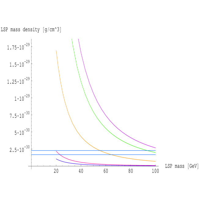
Figure 2:

LSP’s mass density as a function of its mass. The blue, red, yellow, green, violet curves are allowed by  $m_{\widetilde{f}}=50,60,100,160$ GeV, respectively . The horizontal lines are upper and lower experimental limits given in [32].

From Eqs. (30), (31) and (36), it follows that the density increases for increasing of sfermion mass $(\propto m^{2}_{\tilde{f}})$ and decreasing of the LSP mass $(\propto\frac{1}{m_{\tilde{N}}})$. Fig. 2 shows also that the LSP mass is in the range of 100 GeV.

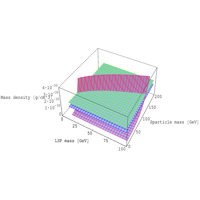
Figure 3:

LSP’s mass density as a function of its mass and sparticle’s one (grid red plane). The grid green plane and grid blue plane correspond to the bounds given in (26).

In Fig. 3, the LSP mass density dependence on two dimensional space of parameters $LSP$ mass and sparticle mass has been plotted. The LSP density is drawn as plane. We have divided the space of parameters into allowed and disallowed regions, where boundaries of acceptable region according to (27) are drawn as grid green plane and grid blue plane. From the Fig. 3, we obtain the lighter sfermion mass is heavier than Bino mass. We also obtain the bounds for mass of the sfermions: $60\ \textrm{GeV}<m_{\widetilde{f}}<130\ \textrm{GeV}$, while the masses of the LSP is in the range of: $20\ \textrm{GeV}<m_{\widetilde{N}}<100\ \textrm{GeV}$. It should be noted that this result coincides with estimation given in [34] (see Fig 1 in page 1114).

Let us consider the case $m_{\widetilde{B}}=m_{\widetilde{f}}$. The LSP mass density has been plotted in Fig. (4). The figure shows that the LSP mass density is very small; it is even smaller than the lower bound given by the [32]. This means that this case is excluded by the WMAP data.

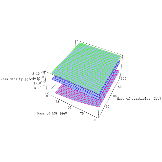
Figure 4:

LSP’s mass density as a function of its mass and sparticle’s one (red plane) in the case $m_{\widetilde{l}}=m_{\widetilde{\widetilde{N}}}$. The grid green plane and grid blue plane correspond to the bounds given in [32].

6 Conclusions

In this paper we have investigated the neutralinos and charginos sector in the supersymmetric economical 3-3-1 model. Accepting conversational assumption such as in the MSSM, eigenmasses and eigenstates in the neutralinos sector were derived. By some circumstance, the LSP is Bino-like state.

In the charginos sector, the mass matrix can be diagonalized by two $5\times 5$ matrices $V$ and $U$.

Assuming that Bino-like is dark matter, its mass density is calculated.

The cosmological dark matter density gives a bound on mass of LSP neutralino is in the range of 20 $\div$ 100 GeV. In addition we have also got a bound on sfermion masses to be: 60 $\div$ 130 GeV. We have also shown that the case $m_{\widetilde{B}}=m_{\widetilde{f}}$ is excluded by the recent experimental WMAP data. Our result is favored the present bound and it should be more cleared in the near future. As in the MSSM, the neutralinos in our model gain the masses in the working region of the LHC. Consequently they could be checked in coming years.

References

- [1] F. Pisano and V. Pleitez, An model for electroweak interactions, Phys. Rev. D 46 (1992) 410; P.H. Frampton, Chiral dilepton model and the flavor question, Phys. Rev. Lett. 69 (1992) 2889; R. Foot et al., Lepton masses in an gauge model, Phys. Rev. D 47 (1993) 4158.
- [2] M. Singer, J.W.F. Valle and J. Schechter, Canonical neutral-current predictions from the weak-electromagnetic gauge group SU(3)U(1), Phys. Rev. D 22 (1980) 738.
- [3] R. Foot, H.N. Long and Tuan A. Tran, and gauge models with right-handed neutrinos, Phys. Rev. D 50 (1994) 34; J.C. Montero et al., Neutral currents and Glashow-Iliopoulos-Maiani mechanism in SU(3)U(1)N models for electroweak interactions, Phys. Rev. D 47 (1993) 2918; H.N. Long, model for right-handed neutrino neutral currents, Phys. Rev. D 54 (1996) 4691; H.N. Long, model with right-handed neutrinos, Phys. Rev. D 53 (1996) 437.
- [4] Y. Okamoto and M. Yasue, Radiatively generated neutrino masses in gauge models, Phys. Lett. B 466 (1999) 267; T. Kitabayshi and M. Yasue, Radiatively induced neutrino masses and oscillations in an gauge model, Phys. Rev. D 63 (2001) 095002; Two-loop radiative neutrino mechanism in an gauge model, Phys. Rev. D 63 (2001) 095006; The interplay between neutrinos and charged leptons in the minimal gauge model, Nucl. Phys. B 609 (2001) 61; permutation symmetry for left-handed and families and neutrino oscillations in an gauge model, Phys. Rev. D 67 (2003) 015006; J.C. Montero, C.A.de S. Pires and V. Pleitez, Neutrino masses through the seesaw mechanism in 3-3-1 models, Phys. Rev. D 65 (2002) 095001; A.A. Gusso, C.A.de S. Pires and P.S. Rodrigues da Silva, Neutrino Mixing and the Minimal 3-3-1 Model, Mod. Phys. Lett. A 18 (2003) 1849; I. Aizawa et al., Bilarge neutrino mixing and -tau permutation symmetry for two-loop radiative mechanism, Phys. Rev. D 70 (2004) 015011; A.G. Dias, C.A.de S. Pires and P.S. Rodriguez da Silva, Naturally light right-handed neutrinos in a 3 3 1 model, Phys. Lett. B 628 (2005) 85; D. Chang and H.N. Long, Interesting radiative patterns of neutrino mass in an model with right-handed neutrinos, Phys. Rev. D 73 (2006) 053006; P.V. Dong, H.N. Long and D.V. Soa, Neutrino masses in the economical 3-3-1 model, Phys. Rev. D 75 (2007) 073006; F. Yin, Neutrino mixing matrix in the 3-3-1 model with heavy leptons and symmetry, Phys. Rev. D 75 (2007) 073010.
- [5] C.A.de S. Pires and O.P. Ravinez, Electric charge quantization in a chiral bilepton gauge model, Phys. Rev. D 58 (1998) 035008; A. Doff and F. Pisano, Charge quantization in the largest leptoquark-bilepton chiral electroweak scheme, Mod. Phys. Lett. A 14 (1999) 1133; Quantization of electric charge, the neutrino, and generation universality, Phys. Rev. D 63 (2001) 097903; P.V. Dong and H.N. Long, Electric Charge Quantization in Models, Int. J. Mod. Phys. A 21 (2006) 6677.
- [6] J.T. Liu and D. Ng, Lepton-flavor-changing processes and CP violation in the model, Phys. Rev. D 50 (1994) 548; J.T. Liu, Generation nonuniversality and flavor-changing neutral currents in the model, Phys. Rev. D 50 (1994) 542; H.N. Long, L.P. Trung and V.T. Van, Rare Kaon Decay in Models, J. Exp. Theor. Phys. 92 (2001) 548, Eksp. Teor. Fiz. 119 (2001) 633; J.A. Rodriguez and M. Sher, Flavor-changing neutral currents and rare B decays in 3-3-1 models, Phys. Rev. D 70 (2004) 117702; C. Promberger, S.S. Schatt and F. Schwab, Flavor-changing neutral current effects and CP violation in the minimal 3-3-1 model, Phys. Rev. D 75 (2007) 115007.
- [7] W.A. Ponce, Y. Giraldo and L.A. Sanchez, Minimal scalar sector of 3-3-1 models without exotic electric charges, Phys. Rev. D 67 (2003) 075001.
- [8] P.V. Dong, H.N. Long, D.T. Nhung and D.V. Soa, model with two Higgs triplets, Phys. Rev. D 73 (2006) 035004.
- [9] P. V. Dong and H. N. Long, The economical model, [arXiv:0804.3239(hep-ph)](2008), to appear in Advances in High Energy Physics.
- [10] P.V. Dong, H.N. Long and D.V. Soa, Higgs-gauge boson interactions in the economical 3-3-1 model, Phys. Rev. D 73 (2006) 075005.
- [11] P.V. Dong, T.T. Huong, D.T. Huong and H.N. Long, Fermion masses in the economical 3-3-1 model, Phys. Rev. D 74 (2006) 053003.
- [12] P.V. Dong et al., in Ref. [4].
- [13] S. Coleman and J. Mandula, All Possible Symmetries of the S Matrix, Phys. Rev. 159 (1967) 1251.
- [14] See, for example, J. Wess and J. Bagger, Supersymmetry and Supergravity, 2nd edition, Princeton University Press, Princeton NJ, (1992); H.E. Haber and G.L. Kane, The search for supersymmetry: Probing physics beyond the standard model, Phys. Rep. 117 (1985) 75.
- [15] S. Martin, A supersymmetry primer, [arXiv:hep-ph/9709356].
- [16] V. Silveira and A. Zee, Scalar Phantoms, Phys. Lett. B 161 (1985) 136; D.E. Holz and A. Zee, Collisional dark matter and scalar phantoms, Phys. Lett. B 517 (2000) 239; C.P. Burgess, M. Pospelov and T. ter Veldhuis, The Minimal Model of nonbaryonic dark matter: a singlet scalar, Nucl. Phys. B 619 (2002) 709; B.C. Bento, O. Bertolami, R. Rosenfeld and L. Teodoro, Self-interacting dark matter and the Higgs boson, Phys. Rev. D 62 (2000) 041302; J. McDonald, Gauge singlet scalars as cold dark matter, Phys. Rev. D 50 (1994) 3637; Thermally Generated Gauge Singlet Scalars as Self-Interacting Dark Matter, Phys. Rev. Lett. 88 (2002) 091304.
- [17] D. N. Spergel and P. J. Steinhardt, Observational Evidence for Self-Interacting Cold Dark Matter, Phys. Rev. Lett. 84 (2000) 3760.
- [18] J.C. Montero, V. Pleitez, M.C. Rodriguez, Supersymmetric 3-3-1 model, Phys. Rev. D 65 (2002) 035006.
- [19] T.V. Duong and E. Ma, Supersymmetric gauge models: Higgs structure at the electroweak energy scale, Phys. Lett. B 316 (1993) 307; Scalar mass bounds in two supersymmetric extended electroweak gauge models, J. Phys G 21 (1995) 159; M.C. Rodriguez, Scalar sector in the minimal supersymmetric 3-3-1 model, Int. J. Mod. Phys. A 21 (2006) 4303.
- [20] J.C. Montero, V. Pleitez and M.C. Rodriguez, Lepton masses in a supersymmetric 3-3-1 model, Phys. Rev. D 65 (2002) 095008; C.M. Maekawa and M.C. Rodriguez, Masses of fermions in supersymmetric models, JHEP 04 (2006) 031.
- [21] M. Capdequi-Peyranere, M.C. Rodriguez, Charginos and neutralinos production at 3-3-1 supersymmetric model in scattering, Phys. Rev. D 65 (2002) 035001.
- [22] Hoang Ngoc Long and Palash B Pal, Nucleon instability in a supersymmetric model, Mod. Phys. Lett. A 13 (1998) 2355.
- [23] J.C. Montero, V. Pleitez and M.C. Rodriguez, Supersymmetric 3-3-1 model with right-handed neutrinos, Phys. Rev. D 70 (2004) 075004.
- [24] D.T. Huong, M.C. Rodriguez and H.N. Long, Scalar sector of supersymmetric model with right-handed neutrinos, [arXiv:hep-ph/0508045].
- [25] P.V. Dong, D.T. Huong, M.C. Rodriguez and H.N. Long, Neutrino masses in the supersymmetric model with right-handed neutrinos, Eur. Phys. J. C 48 (2006) 229.
- [26] R. Martinez, William A. Ponce and Luis A. Sanchez, as an subgroup, Phys. Rev. D 64 (2001) 075013; David L. Anderson and Marc Sher, 3-3-1 models with unique lepton generations, Phys. Rev. D 72 (2005) 095014.
- [27] R. A. Diaz, R. Martinez, J. Alexis Rodriguez , A new supersymmetric gauge model, Phys. Lett. B 552 (2003) 287.
- [28] P.V. Dong, D.T. Huong, M.C. Rodriguez and H.N. Long, Supersymmetric economical 3-3-1 model, Nucl. Phys. B 772 (2007) 150.
- [29] P. V. Dong, D. T. Huong, N. T. Thuy and H. N. Long, Higgs phenomenology of supersymmetric economical 3-3-1 model, Nucl. Phys. B 795 (2008) 361.
- [30] P. V. Dong, Tr. T. Huong, N. T. Thuy and H. N. Long, Sfermion masses in the supersymmetric economical 3-3-1 model, JHEP 11 (2007) 073.
- [31] D. Chang and H.N. Long, in Ref. [4]; See also, M.B. Tully and G.C. Joshi, Generating neutrino mass in the 3-3-1 model, Phys. Rev. D 64 (2001) 011301.
- [32] D. N. Spergel et al. [WMAP Collaboration], Wilkinson Microwave Anisotropy Probe (WMAP) three year results: implications for cosmology. Astrophys. J. Suppl. 170, 377 (2007).
- [33] J. Ellis et al, Supersymmetric relics from the Big Bang, Nucl. Phys. B 238 (1984) 453.
- [34] Particle Data Group collaboration, W.-M. Yao et. al., Review of particle physics, J. Phys. G 33 (2006) 1, p. 114.