Multi-frequency integrated profiles of pulsars

Abstract

We have observed a total of 67 pulsars at five frequencies ranging from 243 to 3100 MHz. Observations at the lower frequencies were made at the Giant Metre Wave Telescope in India and those at higher frequencies at the Parkes Telescope in Australia. We present profiles from 34 of the sample with the best signal to noise ratio and the least scattering. The general ‘rules’ of pulsar profiles are seen in the data; profiles get narrower, the polarization fraction declines and outer components become more prominent as the frequency increases. Many counterexamples to these rules are also observed, and pulsars with complex profiles are especially prone to rule breaking. We hypothesise that the location of pulsar emission within the magnetosphere evolves with time as the the pulsar spins down. In highly energetic pulsars, the emission comes from a confined range of high altitudes, in the middle range of spin down energies the emission occurs over a wide range of altitudes whereas in pulsars with low spin-down energies it is confined to low down in the magnetosphere.

1 Introduction

The frequency dependence of radio emission from pulsars is a key aspect of the emission mechanism. In the radio part of the electromagnetic spectrum, pulsars are known to emit from as low as 10 MHz (Erickson & Mahoney 1985) to at least 150 GHz (Camilo et al. 2007). Radio emission in pulsars is thought to originate from the ultra-relativistic plasma which is streaming out along a group of open magnetic field lines centered around the magnetic poles. The frequency of emission is naturally related to the local plasma conditions, and the frequency dependence of the properties of pulsar emission can be used to probe the active magnetosphere. Since it is not unreasonable to expect that the local plasma conditions change with height above the pulsar surface, it is to some degree expected that observations at different frequencies sample different parts of the open field line region.

It is possible to probe the magnetosphere in two different ways. First, by looking at individual pulses over a wide range of frequencies one can examine the instantaneous, fluctuating properties of the plasma emission (e.g. Karastergiou et al. 2002, Bhat et al. 2007). Secondly, one can determine the long term structure of the magnetic field, the average properties of the magnetic field and the star’s geometry through a study of the time-averaged profiles. These time averaged profiles of pulsars show frequency dependent characteristics which, over the years, have aided our understanding in determining where in the magnetosphere the radio emission arises. Some of these characteristics are: (i) pulsar emission has a steep spectral index with a mean spectral index of $\sim-1.6$ and a large spread in values from 0 to $\sim-4$ (Maron et al. 2000), (ii) pulse profiles appear to widen as the frequency decreases with the implication that the lower frequencies are emitted from higher in the magnetosphere where the flaring of the magnetic field lines is more pronounced (Thorsett 1991, Mitra & Rankin 2002), (iii) different components of the pulse profile have different spectral indices with the more central components appearing to have a steeper spectrum that the outer components. As a consequence, low frequency profiles are often dominated by a single component whereas these components can be flanked by outriders at higher frequencies (Backer 1976, Rankin 1983), (iv) the overall polarization level generally decreases with increasing frequency although in some components polarization can increase.

The most comprehensive multi-frequency observations of pulse profiles were carried out by Gould & Lyne (1998) at frequencies between 234 and 1650 MHz. This database can be supplemented by observations at 100 MHz by the Russian groups (e.g. Izvekova, Malofeev & Shitov 1989; Kuzmin & Losovskii 1999) and at higher frequencies by the Effelsberg (e.g. Kramer et al. 1997; von Hoensbroech & Xilouris 1997) and Parkes (Karastergiou, Johnston & Manchester 2005; Johnston, Karastergiou & Willett 2006) groups.

These observations have been put to good use in constructing beam models for radio pulsars, most notably by Rankin and colleagues (Rankin 1983; Rankin 1993; Mitra & Deshpande 1999; Mitra & Rankin 2002 ) and Lyne & Manchester (1988). The former authors postulate a beam which consists of one or more concentric rings of emission located about the magnetic pole which also produces emission. The latter authors, in contrast, prefer a model where emission regions are located randomly across the polar cap. More recently, Karastergiou & Johnston (2007) have produced an alternative model in which the emission is produced at multiple heights (at a given frequency) and is confined to a region near the last open field lines.

In this paper we present polarization profiles at 5 frequencies (243, 322, 690, 1400 and 3100 MHz) for 34 pulsars, most of which have not been previously observed at the upper and lower frequency end. Section 2 outlines our source selection. The observations were made with the Giant Metre Wave Telescope (GMRT) in India and the Parkes radio telescope in Australia and these are described in detail in Section 3. In Section 4 we present the results and discuss their implications in terms of current models in Section 5.

2 Source Selection

We have embarked on a campaign to produce a database of integrated pulse profiles in full polarization and with high time resolution. At present we have observed close to 400 pulsars at frequencies above 0.6 GHz using the Parkes radio telescope. Profiles from a selection of these pulsars have already been published (Johnston et al. 2005; Karastergiou & Johnston 2006; Johnston et al. 2006; Johnston et al. 2007; Weltevrede & Johnston 2008 ). As the Parkes telescope does not have a good receiver at frequencies below 0.6 GHz, we supplemented the Parkes observations with low frequency observations at the Giant Metre Wave Telescope (GMRT). We selected sources to observe at low frequencies with the following criteria. First, the pulsars should have declinations northwards of $-50$° in order to be visible at the GMRT and southwards of +27° to be visible at Parkes. Secondly, the pulsars must have low dispersion and scattering measures in avoid smearing of the profiles at low frequencies. Finally we needed to choose high flux density pulsars far from the Galactic plane to overcome the high sky brightness temperatures at 200 MHz and the low fluxes of pulsars at high frequencies. This resulted in a sample of 67 pulsars.

3 Observations and Data Analysis

3.1 GMRT Observations

The GMRT observations were carried out in 2007 September spread over 3 days for a total of 30 h. This yielded single pulse polarimetric data for 67 pulsars observed simultaneously at 243, 322 and 607 MHz.

The GMRT is an interferometric array consisting of 30 antennas, each of 45 m diameter, and operates at six different wavebands between 150 and 1450 MHz (Swarup et al. 1991). The array is Y shaped, populated with 14 central antennas in a region of about 1 km², and the remaining 16 are spread along three arms with a longest baseline of 25 km. Polarimetric pulsar observations at the GMRT are done using the phased array mode of operation (see Sirothia 2000, Gupta et al. 2000) where the signals from various antennas are added coherently or in phase. Subsets of 30 antennas can be grouped together to form subarrays operating at different wavebands which gives the flexibility of observing simultaneously at multiple frequencies. The details of the simultaneous, multifrequency, phased array observing technique can be found in Ahuja et al. (2005), Smits et al (2007) and in Bhattacharyya et al. (2007). Here we briefly describe the specifics of the scheme we have employed for our observations.

For our purpose we used three subarrays, with each subarray operating at a centre frequency of 243, 322 and 607 MHz respectively. To minimise the effect of spatial variation of the ionosphere the antennas chosen for 243 MHz were comprised of 8 closely spaced central antennas, for 322 MHz 6 central antennas and one arm antenna were used and for 610 MHz 9 arm antennas were chosen. Each of these wavebands has dual linear feeds which are converted to left and right hand circular via a hybrid. Subsequently two polarization channels of 32 MHz bandwidth are downconverted and further split into upper and lower sideband (USB and LSB) of 16 MHz. The orthogonally polarized complex voltages are then sampled at the Nyquist rate at each antenna. The digitally sampled signals of 16 MHz per polarization channel per sideband is divided into 256 channels by an FX correlator and are added in phase for each polarization. These outputs are fed to the pulsar backend which computes the auto-and cross-polarized power, and is resampled at a rate of 0.512 ms. The backend can be configured to set different values of gains to each spectral channel of each antenna and each polarization before the signals are added using a technique known as bandmasking (see Bhattacharyya et al. 2007 for details). We have this flexibility to assign the first 110 channels (6.87 MHz) of the USB to the 243 MHz subarray, channels 115 - 256 (8.8 MHz) of the USB to the 322 MHz subarray, and the whole 256 channels of the LSB to the 607 MHz subarray. The final time series output has properties equivalent to data recorded using a large single dish and similar polarization calibration methods can be applied to get calibrated Stokes parameters (Johnston 2002, Mitra et al. 2005).

During the observations we did an initial phasing with respect to a reference antenna of each subarray on a strong calibrator source. For observing pulsars, a secondary calibrator source close to the pulsar was used to validate the phasing and if needed phasing was redone. Phasing was done at 1$-$2 hour intervals.

The recorded data were analysed using polarization analysis pulsar software developed at the GMRT. The raw auto-and cross-polarized power were first gain corrected and used to obtain the measured Stokes parameters for the individual spectral channels. For collapsing the channels the fixed delay of the two polarization channels of the reference antenna was corrected along with the pulsar’s dispersion and rotation measure. Observations were made each day of the bright pulsar PSR B1929+10 at a variety of different parallactic angles. From these data, we estimate the error on the linear and circular polarization to be $\sim$5 per cent.

3.2 Parkes Observations

Table 1: Information on the 34 pulsars observed with good signal to noise ratio and low scattering at 243, 327, 690, 1400 and 3100 MHz.

PSR J	PSR B	Period	log($\dot{E}$)	DM	10% Width (degrees)
		(s)	(erg s-1)	(cm-3pc)	243	327	690	1400	3100
J0034$-$0721	B0031$-$07	0.9429	31.3	11.38	41.8	41.1	41.8	36.6	32.0
J0134$-$2937		0.1369	33.1	21.81	35.1	39.1	25.0	17.9	22.9
J0151$-$0635	B0148$-$06	1.4646	30.7	25.66	50.6	41.5	45.0	42.9	40.1
J0152$-$1637	B0149$-$16	0.8327	31.9	11.92	11.7	11.1	11.3	9.8	10.2
J0304+1932	B0301+19	1.3875	31.3	15.74	21.6	21.4	17.0	15.1	14.4
J0525+1115	B0523+11	0.3544	31.8	79.34	27.5	23.9	17.6	17.2	18.9
J0543+2329	B0540+23	0.2459	34.6	77.71	30.0	30.0	23.6	24.3	23.6
J0614+2229	B0611+22	0.3349	34.8	96.91	21.1	17.6	13.4	14.4	13.0
J0630$-$2834	B0628$-$28	1.2444	32.2	34.47	38.1	38.0	38.7	34.4	30.6
J0729$-$1836	B0727$-$18	0.5101	33.7	61.29	24.2	22.4	20.4	19.4	18.9
J0837+0610	B0834+06	1.2737	32.1	12.89	8.4	8.6	9.1	9.1	9.5
J0908$-$1739	B0906$-$17	0.4016	32.6	15.89	23.0	20.2	20.0	20.7	21.2
J0922+0638	B0919+06	0.4306	33.8	27.27	22.7	19.2	16.9	14.8	8.4
J1507$-$4352	B1504$-$43	0.2867	33.4	48.7	11.9	12.7	14.0	13.4	10.2
J1559$-$4438	B1556$-$44	0.2570	33.4	56.1	50.2	22.2	16.5	25.3	28.1
J1645$-$0317	B1642$-$03	0.3876	33.1	35.73	6.2	6.2	6.3	7.4	15.1
J1703$-$3241	B1700$-$32	1.2117	31.2	110.31	24.6	17.1	14.8	14.1	13.4
J1705$-$1906	B1702$-$19	0.2989	33.8	22.91	19.7	17.6	17.2	16.9	16.6
J1709$-$1640	B1706$-$16	0.6530	32.9	24.87	12.7	12.3	13.0	12.0	8.1
J1731$-$4744	B1727$-$47	0.8298	34.0	123.33	15.1	12.2	10.5	10.2	10.9
J1733$-$2228	B1730$-$22	0.8716	30.4	41.14	17.3	34.8	41.1	37.3	40.8
J1735$-$0724	B1732$-$07	0.4193	32.8	73.51	13.4	10.5	16.5	20.4	19.7
J1740+1311	B1737+13	0.8030	32.0	48.67	20.7	20.7	21.8	25.3	24.3
J1745$-$3040	B1742$-$30	0.3674	33.9	88.37	36.6	26.7	19.3	21.2	22.9
J1825$-$0935	B1822$-$09	0.7689	33.7	19.38	9.5	9.8	21.1	21.1	21.4
J1844+1454	B1842+14	0.3754	33.1	41.51	12.0	12.7	24.3	25.0	16.9
J1850+1335	B1848+13	0.3455	33.1	60.15	14.8	16.9	12.0	12.0	11.3
J1900$-$2600	B1857$-$26	0.6122	31.5	37.99	26.7	39.4	38.7	41.1	35.2
J1913$-$0440	B1911$-$04	0.8259	32.5	89.38	7.4	6.0	6.7	8.1	8.4
J1921+2153	B1919+21	1.3373	31.3	12.46	10.5	10.9	11.3	12.7	11.6
J1941$-$2602	B1937$-$26	0.4028	32.8	50.04	10.5	12.4	9.8	12.0	9.8
J2048$-$1616	B2045$-$16	1.9615	31.8	11.46	18.4	17.6	16.2	14.8	13.7
J2116+1414	B2113+14	0.4401	32.1	56.15	16.9	16.2	16.2	18.3	19.0
J2330$-$2005	B2327$-$20	1.6436	31.6	8.46	8.0	7.4	7.0	6.7	6.3

We carried out the observations with the Parkes radio telescope in 2006 August in two separate observing sessions followed by a supplementary session in 2007 December. This resulted in polarization data on more than 250 pulsars with high signal to noise ratio at frequencies of 0.67, 1.4 and 3.1 GHz.

In the first session which took place from 2006 Aug 14 to 17 we used a dual frequency receiver system capable of observing simultaneously in both the 50 and 10 cm bands. We used central frequencies of 3.1 GHz with a bandwidth of 512 MHz and a resolution of 0.5 MHz and 0.69 GHz with an effective bandwidth (after interference rejection) of 35 MHz and a resolution of 0.125 MHz. On-line folding with a digital correlator system resulted in a total of 1024 phase bins per pulse period for each Stokes parameter. Data were recorded to disk at 30 s intervals for a typical observing period of 30 m.

The second session from 2006 August 24 to 27 was conducted with a centre frequency of 1368 MHz, using the H-OH receiver at the prime focus of the Parkes telescope. The total bandwidth was 512 MHz subdivided into 1024 frequency channels in order to remove the effects of interstellar dispersion. Again, 1024 channels were obtained across the band and 1024 phase bins per pulse period per Stokes parameter recorded.

All receivers have orthogonal linear feeds and also have a pulsed calibration signal which can be injected at a position angle of 45° to the two feed probes. An observation of the calibration signal was made prior to every pulsar observation in order to calibrate the polarization and the flux density.

Data analysis was carried out using the PSRCHIVE software package (Hotan, van Straten & Manchester 2004) and the analyis and calibration were carried out in an identical fashion to that described in detail in Johnston et al. (2005). Most importantly, we are able to determine absolute position angles for the linearly polarized radiation at all three of our observing frequencies. We estimate the errors on the linear and circular polarization to be $\sim$2 per cent.

4 Results

Table 1 gives information on the 34 pulsars which had good signal to noise ratio (s/n) at all frequencies and minimal scattering (less than 2°) at the 243 MHz. As scattering is a strong function of observing frequency (with a power-law index of $-4$), this implies that the scattering is less than 1°, and therefore not significant, at the higher frequencies. The table lists the pulsar name, period, spin-down energy ($\dot{E}$) and dispersion measure followed by the width of the profile in degrees measured at 10% of the peak amplitude for each of the five frequencies.

Table 2 lists the 33 pulsars for which weak or no detections were made or the profile was highly scattered so that component features were blurred out at 322 and/or 243 MHz.

Table 2: Pulsars observed with the GMRT but not used in this sample. Y and N denote detections and non-detections.

PSR J	PSR B	243 MHz	327 MHz	Comment
J0108$-$1439		N	Y
J0520$-$2553		Y	Y	Low s/n
J0601$-$0572	B0559$-$05	Y	Y	Scattered
J0624$-$0424	B0621$-$04	Y	Y	Low s/n
J0631+1036		N	N
J0659+1414	B0656+14	N	N
J0738$-$4042	B0736$-$40	N	Y	Scattered
J0742$-$2822	B0740$-$28	Y	Y	Scattered
J1514$-$4834	B1510$-$48	N	Y
J1535$-$4114		N	N
J1536$-$3602		N	N
J1549$-$4848		N	Y
J1557$-$4258		N	Y	Scattered
J1605$-$5257	B1601$-$52	N	N
J1641$-$2347		N	N
J1700$-$3312		N	N
J1740$-$3015	B1737$-$30	N	N
J1743$-$4212		N	N
J1801$-$2920	B1758$-$29	N	Y
J1807$-$0847	B1804$-$08	N	Y	Scattered
J1808$-$0813		N	N
J1820$-$0427	B1818$-$04	Y	Y	Scattered
J1822$-$2256	B1819$-$22	N	Y
J1835$-$1106		N	N
J1848$-$0123	B1845$-$01	N	Y	Scattered
J1852$-$2610		N	N
J1901$-$0906		N	N
J1917+1353	B1915+13	Y	Y	Scattered
J1932+1059	B1929+10	Y	Y	Calibrator
J1935+1616	B1933+16	Y	Y	Scattered
J1937+2544	B1935+25	Y	Y	Low s/n
J2006$-$0807	B2003$-$08	N	Y
J2108$-$3429		Y	Y	Low s/n

PSR J0034$-$0721: The integrated profile of this pulsar is broader at lower frequencies than at higher. It appears that the trailing component gradually declines in intensity with increasing frequency. The fractional polarization remains low at all frequencies. The PA swing varies significantly with frequency. In particular the location of the orthogonal mode jump shifts pulse phase as a function of frequency and is perhaps entirely absent at 4.8 GHz (von Hoensbroech et al. 1998). This is consistent with the idea that the orthogonal modes have different spectral indices (Karastergiou et al. 2005). The geometry of this star has been discussed in detail by Smits et al. (2007).

PSR J0134$-$2937: The frequency evolution of this pulsar is interesting. At frequencies above 600 MHz, the trailing edge of the profile is very sharply defined and the trailing component dominates almost completely. In the 435 MHz profile of Manchester, Han and Qiao (1998) the trailing edge is less sharp and in our 325 MHz profile, not only has the trailing edge been smoothed out, but an unpolarized leading component also appears. The 243 MHz profile has low s/n but again the leading component is apparent. The polarization is high below $\sim$1 GHz but declines thereafter. As noted by Manchester et al. (1998), the PA swing is very shallow. This appears to be a partial cone with the steepest swing of PA occur ahead of the main component.

PSR J0151$-$0635: The profile of this pulsar is a classic double profile, with the two components joined through a saddle or bridge. The profile narrows with increasing frequency and the leading component has the flatter spectral index. It appears as if the steep swing of PA occurs between the two components. At 243 MHz however, the PA traverse is more complicated; the same is seen in the Gould & Lyne (1998) profile. The linear polarization appears to first increase before then decreasing in the leading component. As is common in many of these double pulsars, the polarization fraction is low at the profile edges. The width of the profile decreases with increasing frequency.

PSR J0152$-$1637: This pulsar also has a double profile with the components blended together. There is little evolution with frequency either in the profile width or the relative amplitudes of the two components. The PA swing is complicated by two orthogonal jumps near the leading part of the profile.

PSR J0304+1932: The profile of this pulsar is very similar to that of PSR J0151$-$0635 except that the components are closer together. There is a hint of a central component at the lowest frequencies. There is a significant narrowing of the profile with increasing frequency and the trailing component has the flatter spectral index. Again the steepest swing of PA occurs in the centre of the profile and indeed the PA swing is far less complex than that in either PSR J0151$-$0635 or PSR J0152$-$1637. The pulse width decreases as the frequency increases as does the fractional polarization. The line of sight likely goes close to the magnetic axis (Mitra & Li 2004).

PSR J0525+1115: At face value this pulsar appears to have two prominent and symmetrical components at all frequencies with the leading component having the steeper spectral index. There is a hint of a more central component particularly at 1.4 GHz (see also Weisberg et al. 1999). Also, at the two lowest frequencies there is perhaps a weak trailing component. The circular polarization has a sign change under this central component at 1.4 GHz and higher frequencies. Both Weisberg et al. (1999) and Johnston et al. (2005) took the location of the sign change to be the magnetic pole crossing. However, at 660 MHz and 435 MHz (Weisberg et al. 2004) the circular polarization is confined to the middle of the profile and has no sign change. The linear polarization is at its maximum, with the steepest swing of PA occurring some 3° after the profile midpoint. At still lower frequencies the linear polarization decreases again. There is little, if any, decrease in the overall profile width over this frequency range.

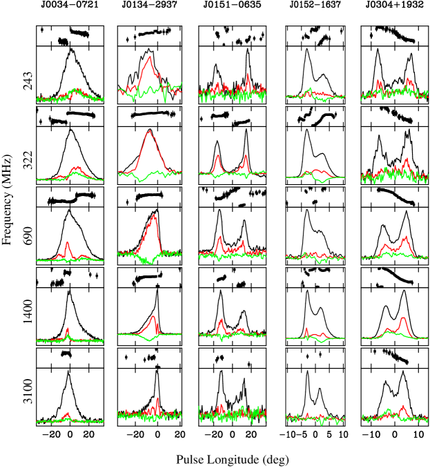
Figure 1: Integrated profiles for 5 pulsars at 5 frequencies. The pulsar name is indicated along the top. The plots show the integrated pulse profiles as a function of longitude for each pulsar. From top to bottom the frequencies are 243, 320, 660, 1400, 3100 MHz. Each plot is subdivided into two panels. The lower plot shows the total intensity (black line), linear polarization (red line) and circular polarization (green line) as a function of pulse longitude. The top panel shows the position angle of the linearly polarized radiation and runs between $-90$° and +90°.

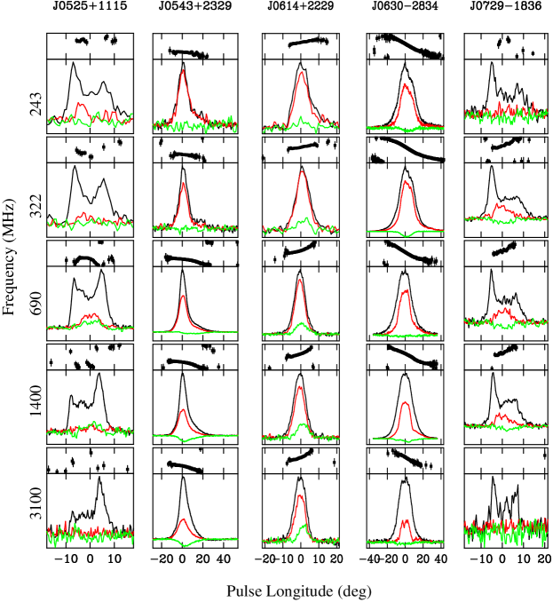
Figure 2: Integrated profiles for 5 pulsars at 5 frequencies as marked. See Figure 1 for details.

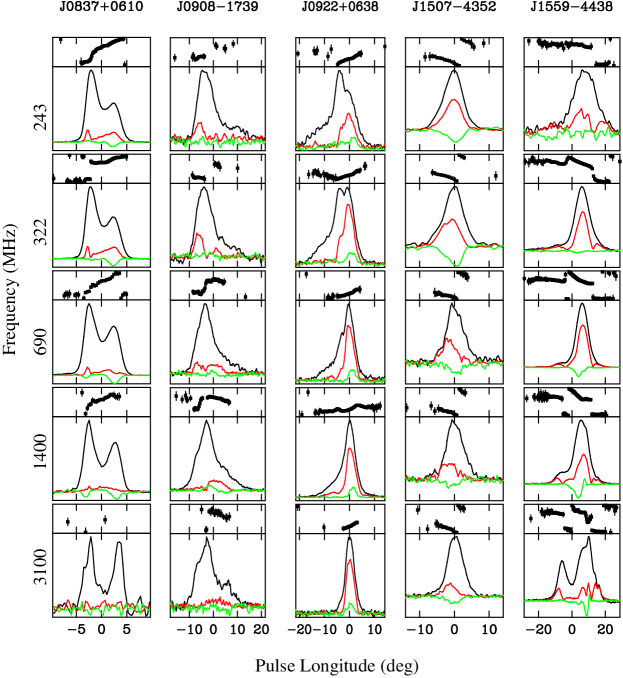
Figure 3: Integrated profiles for 5 pulsars at 5 frequencies as marked. See Figure 1 for details.

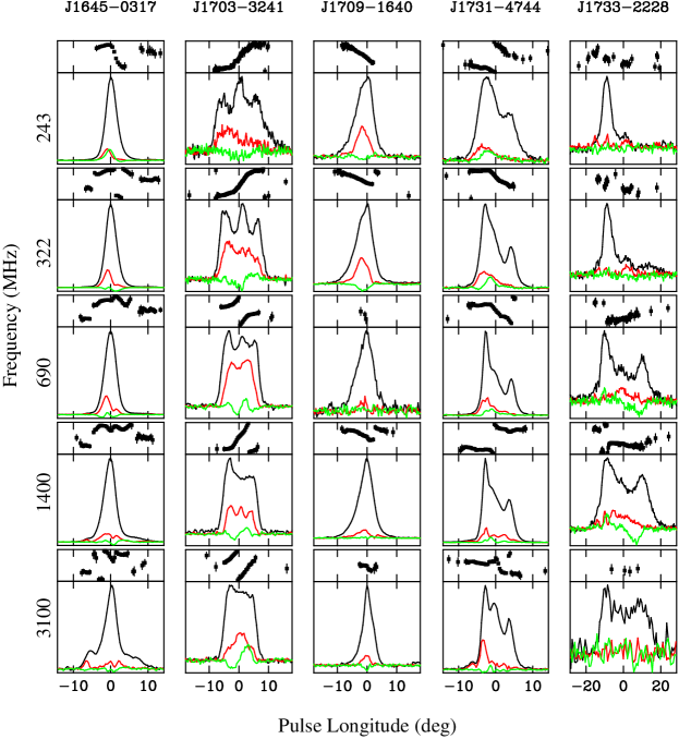
Figure 4: Integrated profiles for 5 pulsars at 5 frequencies as marked. See Figure 1 for details.

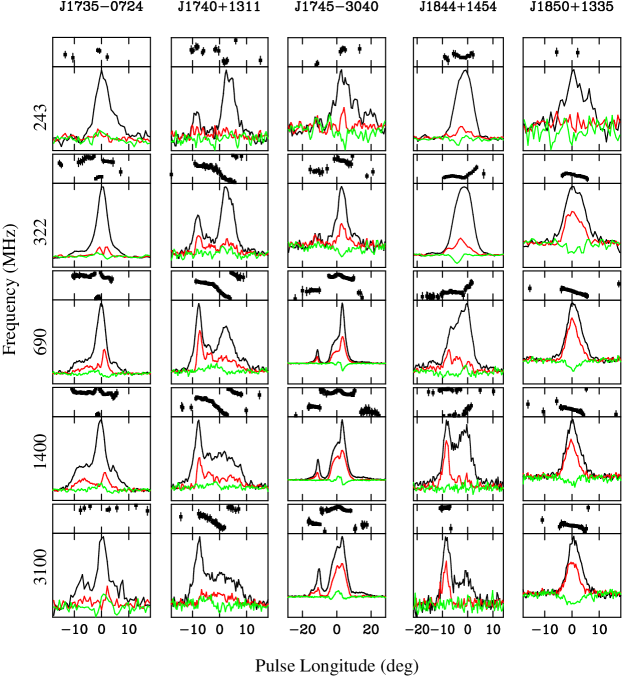
Figure 5: Integrated profiles for 5 pulsars at 5 frequencies as marked. See Figure 1 for details.

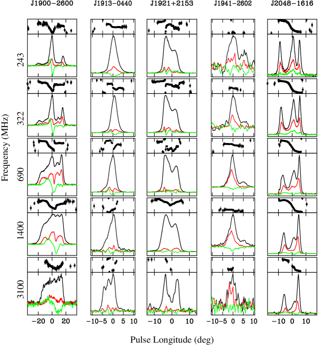
Figure 6: Integrated profiles for 5 pulsars at 5 frequencies as marked. See Figure 1 for details.

PSR J0543+2329: The profile from this pulsar appears to come from the leading edge of the beam (Lyne & Manchester 1988). The PA clearly steepens towards later longitudes (see the discussion in Johnston et al. 2007). The profile width declines with frequency as the trailing edge becomes sharper. The main change is that the linear polarization decreases with increasing frequency whereas the circular polarization slowly increases (as is seen in a number of other pulsars; see von Hoensbroech & Lesch 1999).

PSR J0614+2229: This pulsar is similar to the previous one. There is a single, highly linearly polarized component at all frequencies. The PA swing is rather flat but appears to steepen towards the trailing edge of the profile. Again, the pulse width decreases with frequency as the trailing edge becomes sharper. There is a slow decline in the fractional polarization with frequency.

PSR J0630$-$2834: The profile of this pulsar consists of a single broad component with a full width of $\sim$40°. The swing of PA is steepest at the component centre at all frequencies. This indicates that there is not much difference in emission height between the lowest and highest frequencies. The pulse width and linear polarization decline slowly with increasing frequency, a trend which continues up to 8.4 GHz.

PSR J0729$-$1836: The profile consists of a narrow leading component and a broader trailing component. The profile gets narrower with increasing frequency and the polarization fraction declines but otherwise shows little change. The PA swing shows an orthogonal jump near the start of the profile and has a linear slope with no obvious steepening. At 3.1 GHz the pulsar is weak and the polarization has disappeared.

PSR J0837+0610: The pulse profile consists of two blended components with an overall width of only $\sim$9°, a width which appears to increase at higher frequencies. The leading component has the steeper spectral index. The linear polarization profile also largely remains constant with frequency. The PA swing is highly frequency dependent.

PSR J0908$-$1739: The pulse profile consists of a steep rising edge and a shallower trailing edge with the hint of an extra trailing component in the wings of the profile. There is little variation in pulse structure or width as a function of frequency. Linear polarization is seen against the leading edge at low frequencies and more towards the centre of the profile at higher frequencies. The PA swing is unclear due to the presence of orthogonal mode jumps. The emission is likely to arise from the leading edge of the beam only (Lyne & Manchester 1988).

PSR J0922+0638: The profiles of this pulsar at various frequencies have been discussed at length in Weisberg et al. (1999). In that paper, the authors noted that the profile appeared to bifurcate at 435 MHz but that no lower frequency profiles were available. We can confirm the presence of a low frequency component here. In the figure we have aligned the profile on the trailing edge which corresponds to a location of high linear polarization and positive circular polarization. Already at 660 MHz a hint of the bifurcated component can be seen, and this component starts to dominate the profile at 243 MHz. In addition to this new component there is also a pedestal-like leading component which is somewhat stronger at lower frequencies. The polarization swing is shallow across the polarized part of the profile. This is likely to be a partial cone where only the trailing edge is seen. The pulse width declines strongly with increasing frequency as the leading edge becomes sharper.

PSR J1507$-$4352: The profile of this pulsar consists of a single narrow component at all frequencies. There is some narrowing of the profile towards higher frequencies. The linear polarization fraction shifts away from the pulse centre towards the leading edge as the frequency increases and the fractional polarization decreases. The PA gradient is almost constant across the pulse.

PSR J1559$-$4438: The profiles of this pulsar at 0.69 GHz and above were discussed in detail in Johnston et al. (2007). In that paper we remarked on the strong frequency evolution between 1.4 and 3.1 GHz. At 322 MHz the profile is similar to that at 690 MHz although the circular polarization is almost absent. At 243 MHz some scatter broadening is seen which flattens the PA swing and has reduced the amount of linear polarization.

PSR J1645$-$0317: This pulsar has a ‘classical’ variation of pulse profile with frequency. At low frequencies the profile consists of a single component. At frequencies above 1 GHz, outrider components are seen flanking the main component and these become very prominent at 5 GHz (von Hoensbroech & Xilouris 1997). The linear polarization remains low at all frequencies. The PA swing is rather confusing. There is an orthogonal jump against both the leading and trailing outriders and in the middle of the profile the PA takes a strange dip from its otherwise slow increase. At 243 MHz however, the PA swings steeply following the profile peak, with a lag of about 1.5°. This is not seen in the lower time resolution profile of Gould & Lyne (1998). The pulse width is very narrow but increases with increasing frequency as the outriders appear.

PSR J1703$-$3241: This is a beautiful example of a triple profile pulsar. The central component has the steepest spectral index and is much less prominent at high frequencies. The profile gradually narrows with increasing frequency. The PA swing is steepest through the centre of the profile. The linear polarization is moderately high and the circular polarization changes hand in the centre of the profile.

PSR J1705$-$1906: The profile of this pulsar consists of a main pulse and an interpulse separated almost exactly by 180° (Biggs et al. 1988, Weltevrede et al. 2007). The main pulse consists of two components, each highly polarized at low frequencies but with the leading component less so at high frequencies. The circular polarization is negative on the leading edge but changes sign towards the trailing edge. The interpulse is barely visible at low frequencies but reaches about half the amplitude of the main pulse at higher frequencies. However, this amplitude again declines at still higher frequencies. The interpulse is virtually 100% polarized. The width of the main pulse decreases with increasing frequency.

PSR J1709$-$1640: The pulse profile does not vary much as a function of frequency except for a slight narrowing. In the higher signal to noise profiles, an orthogonal jump can be seen just after the centre of the pulse profile. At 3.1 GHz the PA swing has lost its RVM nature and the polarized fraction is substantially lower than at lower frequencies.

PSR J1731$-$4744: At low frequencies the profile of this pulsar consists of two components with the first having some linear and circular polarization. As the frequency increases, the pulse width slowly decreases and a more centrally located component emerges. At 3.1 GHz the central component is quite prominent and it also disrupts the rather smooth PA swing seen at lower frequencies. The prominence of the central component at higher frequencies is contrary to that seen in other triple pulsars and a further example of this is seen in the next object.

PSR J1733$-$2228: The frequency evolution of this profile is very interesting. At 243 MHz it consists of single dominant component followed by a weak component. At 322 MHz a third, trailing component appears in the profile. At 0.69 and 1.4 GHz, the central and trailing components are more prominent relative to the leading component and the profile looks like a classical triple profile with a swing of circular polarization through the centre. At the highest frequency the profile has become boxy. It is hard to tell from the PA swing where the magnetic pole crossing might be located.

PSR J1735$-$0724: The profile evolution of this pulsar mirrors that of PSR J1645$-$0317. At high frequencies the central component is flanked by two outrider components which become much less prominent at lower frequencies. As with PSR J1645$-$0317, linear polarization is low and the PA swing exhibits a curious deviation from a slow swing in the centre of the profile, apparently related to the narrow component of linear polarization seen clearly at 322 and 690 MHz. The pulse width increases with frequency.

PSR J1740+1311: The pulse profile of this pulsar has been presented with very high s/n at 408 and 1400 MHz by Weisberg et al. (1999) and Weisberg et al. (2004). At the lower frequency, 5 clear components can be seen (especially in linear polarization). The midpoint of the profile also coincides with the steepest PA swing (Johnston et al. 2005). The 3.1 GHz profile is similar to the 1.4 GHz profile except for a reduction in the linear polarization. Kijak et al. appear to show the central component re-appearing at 4.8 GHz. At 243 MHz we still can observe the leading component whereas in the 227 MHz observations of Hankins & Rickett (1986) it appears to be absent as is also the case in the 102 MHz profile of Izvekova et al. (1989). The profile width appears to increase with frequency.

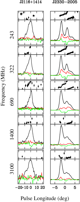
Figure 7: Integrated profiles for 2 pulsars at 5 frequencies as marked. See Figure 1 for details.

PSR J1745$-$3040: The profile undergoes significant frequency evolution which is similar to that in PSR J1559$-$4438. At 3.1 GHz there is a strong leading component, followed by a main component consisting of two nearly equal components and a low ampltiude trailing component. As the frequency decreases, so does the relative amplitude of the leading component and the leading component of the main pulse. At 322 MHz only the merest hint of the leading component is still present and at 243 MHz a possible weak trailing component appears. At high frequencies the PA swing is complex with an initial orthogonal jump followed by a W shaped PA curve which has been distorted in the pulse centre. The fraction of linear polarization also appears to increase with increasing frequency.

PSR J1825$-$0935: This peculiar pulsar has been the subject of much debate in the literature. The profile consists of a double component followed some 180° later by an interpulse and it appears as if the interpulse and the leading component of the main pulse exchange information (Gil et al. 1994). Attempts have been made to understand the geometry of this pulsar, most recently by Dyks et al. (2005). Although a 100 MHz observation of the main pulse has been published (Izvekova et al. 1989), no published profile of the interpulse exists below 400 MHz. In both our 243 and 322 MHz profile the interpulse is clearly present with the same separation from the main pulse as seen at higher frequencies. At 243 and 322 MHz the leading component of the main pulse and the interpulse is very weak. Although the leading component retains its polarization as the frequency increases, it decreases substantially in the trailing component.

PSR J1844+1454: Strong profile evolution is seen in this pulsar. At 3.1 GHz, the profile consists of a strong, narrow leading component which is highly polarized followed by a weaker, broader trailing component with little polarization. At 1.4 GHz these components are nearly equal amplitude. A steep swing of PA can be seen towards the trailing edge of the profile. At 0.69 GHz the leading component is dominated by the trailing component which completely takes over at yet lower frequencies. As a result, the pulse width increases, reaching a maximum at 1.4 GHz before decreasing again.

PSR 1850+1335: The profile consists of a single component at all frequencies. There is a small amount of pulse broadening at the lower frequencies. The polarization is moderately high, except at 243 MHz where little or no polarization is seen. There is a linear gradient of PA across the pulse indicating a line of sight relatively far from the magnetic axis. The pulse width decreases with frequency.

PSR 1900$-$2600: The profile of this pulsar shows significant frequency evolution and there are clearly a large number of independent components in the profile each with a different spectral index. At the lowest frequency a strong central component dominates with weak outriders flanking it. As the frequency increases the outriders become stronger compared to the central component. At 1.4 GHz at least 5 different components can be discerned and the profile has become boxy at 3.1 GHz. The overall pulse width remains largely constant with frequency. A swing in the sense of the circular polarization can be seen across the centre of the profile at all frequencies. As expected for a complex profile the PA swing is significantly disturbed from that expected in any simple geometric model.

PSR 1913$-$0440: The profile of this pulsar evolves from a simple single component at the lowest frequency to a triple component pulsar at 3.1 GHz. The component at low frequencies can be most readily identified with the trailing component at high frequencies. The fraction of linear polarization is low and the PA traverse is peculiar and not consistent between frequencies. At 0.69 and 1.4 GHz it appears to sharply rise towards the trailing edge of the profile. At 322 and 243 MHz, in contrast, the PA swing appears to be flat across the trailing edge yet drops sharply through the pulse centre.

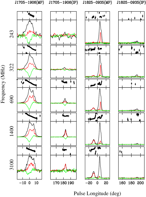
Figure 8: Integrated profiles for the main pulse and interpulse of PSR J1705$-$1906 and PSR J1825$-$0935 at 5 frequencies as marked. The scale on the main and interpulse plots are the same. See Figure 1 for details.

PSR J1921+2153: The profile of this, the first pulsar discovered, is rather unusual. It consists of two blended components with likely a central component also present. The spectral index of the outer two components is similar and flatter than that of the central component which has all but disappeared by 3.1 GHz. Weisberg et al. (1999) discuss the presence of a further leading component seen at 1.4 GHz which is also evident in our observations (see also Johnston et al. 2005). However, this component is not present at any lower frequency. At 3.1 GHz, however, in spite of the low s/n, it appears as if this leading component has become stronger. The profile width is relatively constant with frequency. The PA swing at all frequencies is complicted by orthogonal mode jumps and component blending.

PSR 1941$-$2602: At 243 MHz the profile of this pulsar consists of a dominant leading component and a weaker trailing component. The spectral index of the trailing component is steeper than that of the leading component so that, at 3.1 GHz the trailing component is barely visible. The linear polarization appears to increase with increasing frequency. The PA swing is flat throughout and the overall width remains fairly constant. This may also be a partial cone, with emission seen only from the leading edge of the beam.

PSR 2048$-$1616: The pulse profile of this strong pulsar has had a variety of interpretations over the years (e.g. most recently by Mitra & Li 2004 and Johnston et al. 2007). In brief, the profile shows three major components, of which the central one has the steepest spectral index. However, the central component is not located mid-way between the two outer components but lies more on the trailing side. It also lags the steepest swing of PA. At 243 MHz there is a hint that a further central component is emerging on the leading side. The profile at 102 MHz in Izvekova et al. (1989) is peculiar as it only consists of two components; a high signal-to-noise ratio profile at these low frequencies would be very useful. The pulse width decreases with increasing frequency as does the fractional polarization.

PSR 2116+1414: The profile consists of a single component which has a steeper trailing edge than a leading edge. The profile width remains constant with frequency or perhaps increases slightly. The fractional polarization is low at all frequencies.

PSR 2330$-$2005: The profile of this pulsar consists of three components. At 243 MHz the leading component dominates followed by the central and lagging component. The middle component has the steepest spectral index and it is much less prominent at 3.1 GHz. The overall pulse width is only marginally greater at 243 MHz than at 3.1 GHz but appears to decrease monotonically with increasing frequency. The linear polarization fraction is moderately high at low frequencies but has declined significantly by 3.1 GHz. In Johnston et al. (2007) we surmised that there was a steep swing of PA across the central component rather than an orthogonal jump. This is borne out by the 243 MHz PA traverse which shows a continuous rise in the PA.

5 Discussion

Although we did not attempt to choose a representative sample of pulsars as part of our selection criteria, we can see from the pulse profiles that many of the typical characteristics of pulsars are on display. In this section, we compare these objects to the various paradigms of pulsar phenomenology which have become integral in any attempt to understand pulsar radio emission.

5.1 Frequency Evolution of Profiles

Clearly, the integrated profiles of pulsars vary as a function of frequency, sometimes mildly, sometimes dramatically. In virtually all the pulse profiles presented here, however, individual components are present at all frequencies to a greater or lesser degree. In our sample, only PSRs J1645$-$0317, J1844+1454 and J1913$-$0440 show features at high frequency not present at 243 MHz.

It has been evident for many years that some form of radius-to-frequency mapping occurs within the pulsar magnetosphere and that lower frequencies are emitted from higher in the magnetosphere than high frequencies. However, in the range 0.1 to 10 GHz or so, the effect is not large and the bulk of the radio pulsars emit from a rather narrow range of altitudes from low down in the magnetosphere. In contrast, the variation in height seen in different components of a pulsar at a given frequency can be rather large with the outer components having higher emission heights than more central components (Gupta & Gangadhara 2003).

Radius-to-frequency mapping should therefore be clearest in the simplest profiles, without the complicating effects of individual component spectral index. Indeed, in the simple profiles of our sample, a general narrowing of the pulse width of between 20 and 30 per cent is observed from 240 to 3100 MHz, as seen in other studies (e.g. Thorsett 1991). However almost one-third of our sample shows the profile width increasing with frequency, opposite to that expected. An explanation for this apparent anomaly can be sought in the fact that components towards the outside of the profile increase in relative amplitude with frequency, causing the apparent pulse broadening (see Table 1). To investigate the true wdith evolution with frequency it becomes necessary to trace the profiles out to very low signal levels (Kijak & Gil 1997), a task not possible with our dataset.

5.2 Polarization Evolution

In the standard picture of pulsar emission, the degree of polarization generally decreases with increasing frequency. A physical explanation of this phenomenon is not straightforward (von Hoensbroech, Lesch & Kunzl 1998) but may simply be related to the fact that the high frequency radiation traverses more of the magnetosphere than the low frequency emission.

Although the general decrease of linear polarization with frequency is seen in many of our pulsars, we can identify further trends seen in subgroups of sources. For instance, a number of highly polarized profile components remain highly polarized at high frequencies (e.g. for PSR J0922+0638). In some pulsars, the change in the degree of polarization is not monotonic with frequency (e.g. PSRs J0922+0638, J1703$-$3241 and J1844+1454). Generally speaking, simple profiles are more likely to be characterized by high linear polarization than complex profiles and individual components within a given pulsar can behave differently with frequency.

We can interpret the depolarization of the emission in two possible ways, the first of which is a geometric rather than a physical effect and the second which involves orthogonally polarized modes. It is likely that both effects are important because even in pulsars where no obvious orthogonal jumps are seen, depolarization is still observed as the frequency increases. In the first interpretation, the high degree of polarization arises from the fact that the emission is forced to travel along the field lines with a high Lorentz factor, $\gamma$. The detected radiation has a duration proportional to $1/\gamma$, typically shorter than the data sampling rate, so that several emission bursts are (incoherently) summed in the detector. This results in a decrease in the polarization fraction. At high frequencies, which arise from lower in the pulsar magnetosphere, the squeezing together of the field lines exacerbate this effect and result in reduced degree of polarization. This is a geometrical effect, and in principle, can be overcome by higher sampling rates. The second idea, discussed in detail in Karastergiou et al. (2005), involves the interaction of the two orthogonally polarized modes of emission present in the magnetospheric plasma (Manchester, Taylor & Huguenin 1975). In our simple model, the two orthogonally polarized modes had different spectral indices, and the fractional polarization seen in a given component depended on the relative strengths of the two modes. Some observational evidence in support of this model comes from the fact that highly polarized pulsars (or components) also appear to have flatter spectral indices (see also von Hoensbroech, Kijak & Krawczyk 1998).

In addition to the degree of linear polarization, the dependence of the PA swing with frequency in our sample is very interesting. In general, the PA traverse is highly frequency dependent, whereas in the simple geometrical explanation it should be independent of frequency (Radhakrishnan & Cooke 1969). The PA at a given longitude is therefore highly modulated by processes in the magnetosphere, in particular the occurrence of orthogonal mode jumps and, most likely, the presence of overlapping components at different emission heights. A clear example of this is PSR J1559$-$4438. At 322 MHz, the PA swing is well behaved and the linear polarization is high. At 3.1 GHz, in contrast, the linear polarization is lower, several new components are emerging and the PA swing has become horribly complicated. In contrast, pulsars with high levels of linear polarization and generally simple profiles tend to show PA swings which closer resemble the geometrical paradigm of the rotating vector model (e.g. PSR J0630$-$2834).

5.3 Classification

The most common pulse-profile classification schemes depend on the number of components that constitute the profile, their behaviour with frequency and their polarization characteristics.

A glance at the pulsars in our sample shows that they contain most of the well-defined pulsar types. In particular, 8 pulsars (PSRs J0151$-$0635, J0152$-$1637, J0304+1932, J0525+1115, J0729$-$1836, J0837+0610, J1705$-$1906 (main pulse), J1921+2153) would be classifed as ‘double’ in the scheme of Rankin (1983). Their profiles are all two-humped with each component being the same width, they show little profile evolution with frequency except for profile narrowing, they generally have low polarization and the PA swing is steepest at or near the profile centre. In the main, they tend to be long period pulsars, with periods 1 s or above, they have low values of $\dot{E}$ and their profile width is less than 20°. The simplest interpretation is that the observational profile arises from a cone of emission located at a low altitude ($<300$ km) and close to the last open field lines.

Other pulsars seem to fall into the ‘partial cone’ category defined by Lyne & Manchester (1988). These are PSRs J0134$-$2937, J0543+2329, J0614+2229, J0908$-$1739, J0922+0638 and perhaps J1941$-$2602. These pulsars have a sharp outer edge (either leading or trailing) and a smoother inner edge which becomes steeper at high frequencies. Polarization is high and the PA swing appears to steepen where the total intensity emission runs out. The periods of these pulsars tend to be near 0.5 s, and they also have spin-down energies intermediate between the highly energetic young objects and the low $\dot{E}$ pulsars. The interpretation of these pulsars are that their emission arises from a cone which is only partially illuminated and so (by chance) only the leading or trailing edge is seen. Interestingly, the measured pulse widths of these pulsars are already larger than those of the doubles in spite of the fact that only half the profile is seen. This implies their emission arises from significantly higher in the magnetosphere than those of the doubles.

Finally there are some pulsars which one might conveniently shoehorn into some classification but which, for the most part, have bizarre enough behaviour that many different interpretations could be made. These are PSRs J1559$-$4038, J1733$-$2228, J1740+1311, J1745$-$3040, J1844+1454 and J1913$-$0440. One feature which they all have in common is that their PA swing contains many features and are highly distorted compared to expectations from geometrical models. In the context of the Karastergiou & Johnston (2007) model, this arises because the multiple components in these complex profiles all arise from different emission heights.

5.4 Time Evolution of Pulse Profiles?

We can draw several strands of the above sub-sections together. Observationally it is known that the young highly energetic pulsars (with $\dot{E}>10^{35}$ ergs^-1) have simple, highly polarized profiles which are formed relatively high in the pulsar magnetosphere (e.g. Johnston & Weisberg 2006). There are no young, high $\dot{E}$ pulsars in this sample, mainly because of the difficulty in observing them at low frequencies. These pulsars lie at low galactic latitudes and have high dispersion and scattering measures. The combination of high sky background temperature and high scattering renders the majority of young pulsars undetectable below $\sim$1 GHz.

In our sample here, we see that many pulsars have complex profiles with many components, low to medium polarization and severe disruption of the PA swing especially in the centre of the profiles. These have a mean $\dot{E}$ of 10^32.6 ergs^-1 and also appear to originate from relatively high in the magnetosphere. Finally, at least a subset of the lowest $\dot{E}$ pulsars have narrow double profiles, low polarization and a more geometric PA swing. Their mean $\dot{E}$ is 10^32.1 ergs^-1 and emission likely occurs low in the magnetosphere.

We therefore hypothesise a possible time evolution sequence for pulsar profiles, consistent with the ideas initially presented in Rankin (1993) and subsequently modified in Karastergiou & Johnston (2007), and manifesting itself as different profile types for different values of $\dot{E}$. The high $\dot{E}$ pulsars have relatively simple profiles arising from a single cone of emission high in the pulsar magnetosphere. As they spin down, the range of emission heights increases, producing complex profiles (including partial cones) and non-geometrical PA swings. Finally, many low $\dot{E}$ pulsars show profiles consistent with a single emission cone at a rather low height.

A greater degree of linear polarization generally arises from components located high in the magnetosphere. For low $\dot{E}$ pulsars this generally implies low frequencies; hence the polarization declines rapidly with increasing frequency. For high $\dot{E}$ pulsars, however, with higher emission heights, the profiles remain polarized up to much higher frequencies.

6 Conclusions

The combination of the GMRT and Parkes capabilities has allowed us to create a high time resolution, full Stokes parameterization of 34 pulsars at frequencies between 240 and 3100 MHz. We have presented their profiles and provided a succint description of each pulsar’s characteristics.

The general ‘rules’ of pulsar profiles are seen in these data; the profiles narrow with frequency, outer components are more prominent at higher frequencies and the polarization fraction declines with frequency.

We surmise that the emission in high $\dot{E}$ pulsars arises from a high height in the magnetosphere, that moderate $\dot{E}$ pulsars have highly complex profiles and PA swings due to a large range of possible emission heights and that at least a subset of low $\dot{E}$ pulsars have simpler emission beams from a relatively low height.

References

- Ahuja et al. (2005) Ahuja A. L., Gupta Y., Mitra D., Kembhavi A. K., 2005, MNRAS, 357, 1013
- Backer (1976) Backer D. C., 1976, ApJ, 209, 895
- Bhat et al. (2007) Bhat N. D. R., Gupta Y., Kramer M., Karastergiou A., Lyne A. G., Johnston S., 2007, A&A, 462, 257
- Bhattacharyya et al. (2008) Bhattacharyya B., Gupta Y., Gil J., 2008, MNRAS, 383, 1538
- Biggs et al. (1988) Biggs J. D., Lyne A. G., Hamilton P. A., McCulloch P. M., Manchester R. N., 1988, MNRAS, 235, 255
- Camilo et al. (2007) Camilo F., Ransom S. M., Peñalver J., Karastergiou A., van Kerkwijk M. H., Durant M., Halpern J. P., Reynolds J., Thum C., Helfand D. J., Zimmerman N., Cognard I., 2007, ApJ, 669, 561
- Dyks et al. (2005) Dyks J., Zhang B., Gil J., 2005, ApJ, 626, L45
- Erickson & Mahoney (1985) Erickson W., Mahoney M., 1985, ApJ, 299, L29
- Gil et al. (1994) Gil J. A., Jessner A., Kijak J., Kramer M., Malofeev V., Malov I., Seiradakis J. H., Sieber W., Wielebinski R., 1994, A&A, 282, 45
- Gould & Lyne (1998) Gould D. M., Lyne A. G., 1998, MNRAS, 301, 235
- Gupta & Gangadhara (2003) Gupta Y., Gangadhara R. T., 2003, ApJ, 584, 418
- Gupta et al. (2000) Gupta Y., Gothoskar P., Joshi B. C., Vivekanand M., Swain R., Sirothia S., Bhat N. D. R., 2000, in Kramer M., Wex N., Wielebinski R., eds, Pulsar Astronomy - 2000 and Beyond, IAU Colloquium 177 Astronomical Society of the Pacific, San Francisco
- Hankins & Rickett (1986) Hankins T. H., Rickett B. J., 1986, ApJ, 311, 684
- Hotan et al. (2004) Hotan A. W., van Straten W., Manchester R. N., 2004, PASA, 21, 302
- Izvekova et al. (1989) Izvekova V. A., Malofeev V. M., Shitov Y. P., 1989, Sov. Astron., 33, 175
- Johnston (2002) Johnston S., 2002, PASA, 19, 277
- Johnston et al. (2005) Johnston S., Hobbs G., Vigeland S., Kramer M., Weisberg J. M., Lyne A. G., 2005, MNRAS, 364, 1397
- Johnston et al. (2006) Johnston S., Karastergiou A., Willett K., 2006, MNRAS, 369, 1916
- Johnston et al. (2007) Johnston S., Kramer M., Karastergiou A., Hobbs G., Ord S., Wallman J., 2007, MNRAS, 381, 1625
- Johnston & Weisberg (2006) Johnston S., Weisberg J. M., 2006, MNRAS, 368, 1856
- Karastergiou & Johnston (2006) Karastergiou A., Johnston S., 2006, MNRAS, 365, 353
- Karastergiou & Johnston (2007) Karastergiou A., Johnston S., 2007, MNRAS, 380, 1678
- Karastergiou et al. (2005) Karastergiou A., Johnston S., Manchester R. N., 2005, MNRAS, 359, 481
- Karastergiou et al. (2002) Karastergiou A., Kramer M., Johnston S., Lyne A. G., Bhat N. D. R., Gupta Y., 2002, A&A, 391, 247
- Kijak & Gil (1997) Kijak J., Gil J., 1997, MNRAS, 288, 631
- Kramer et al. (1997) Kramer M., Xilouris K. M., Jessner A., Lorimer D. R., Wielebinski R., Lyne A. G., 1997, A&A, 322, 846
- Kuz’min & Losovskii (1999) Kuz’min A. D., Losovskii B. Y., 1999, Astronomy Reports, 43, 288
- Lyne & Manchester (1988) Lyne A. G., Manchester R. N., 1988, MNRAS, 234, 477
- Manchester et al. (1998) Manchester R. N., Han J. L., Qiao G. J., 1998, MNRAS, 295, 280
- Manchester et al. (1975) Manchester R. N., Taylor J. H., Huguenin G. R., 1975, ApJ, 196, 83
- Maron et al. (2000) Maron O., Kijak J., Kramer M., Wielebinski R., 2000, A&AS, 147, 195
- Mitra & Deshpande (1999) Mitra D., Deshpande A. A., 1999, A&A, 346, 906
- Mitra & Li (2004) Mitra D., Li X. H., 2004, A&A, 421, 215
- Mitra & Rankin (2002) Mitra D., Rankin J. M., 2002, ApJ, pp 322–336
- Radhakrishnan & Cooke (1969) Radhakrishnan V., Cooke D. J., 1969, Astrophys. Lett., 3, 225
- Rankin (1983) Rankin J. M., 1983, ApJ, 274, 333
- Rankin (1993) Rankin J. M., 1993, ApJ, 405, 285
- Sirothia (2000) Sirothia S., 2000, PhD thesis, University of Pune
- Smits et al. (2007) Smits J. M., Mitra D., Stappers B. W., Kuijpers J., Weltevrede P., Jessner A., Gupta Y., 2007, A&A, 465, 575
- Swarup et al. (1991) Swarup G., Ananthakrishnan S., Kapahi V. K., Rao A. P., Subrahmanya C. R., Kulkarni V. K., 1991, Current Science, 60, 95
- Thorsett (1991) Thorsett S. E., 1991, ApJ, 377, 263
- von Hoensbroech et al. (1998) von Hoensbroech A., Kijak J., Krawczyk A., 1998, A&A, 334, 571
- von Hoensbroech & Lesch (1999) von Hoensbroech A., Lesch H., 1999, A&A, 342, L57
- von Hoensbroech et al. (1998) von Hoensbroech A., Lesch H., Kunzl T., 1998, A&A, 336, 209
- von Hoensbroech & Xilouris (1997) von Hoensbroech A., Xilouris K. M., 1997, A&AS, 126, 121
- Weisberg et al. (2004) Weisberg J. M., Cordes J. M., Kuan B., Devine K. E., Green J. T., Backer D. C., 2004, ApJS, 150, 317
- Weisberg et al. (1999) Weisberg J. M., Cordes J. M., Lundgren S. C., Dawson B. R., Despotes J. T., Morgan J. J., Weitz K. A., Zink E. C., Backer D. C., 1999, ApJS, 121, 171
- Weltevrede & Johnston (2008) Weltevrede P., Johnston S., 2008, MNRAS, Submitted.
- Weltevrede et al. (2007) Weltevrede P., Wright G. A. E., Stappers B. W., 2007, A&A, 467, 1163