Coulomb gauge approach to scalar hadrons

Abstract

The Coulomb gauge model, involving an effective QCD Hamiltonian in the Coulomb gauge, is applied to scalar hadrons. Mass predictions are presented for both conventional $q{\bar{q}}$ meson and $q{\bar{q}}q{\bar{q}}$ tetra-quark states. Mixing matrix elements between these states were also computed and diagonalized to provide a reasonable description of the scalar spectrum below 2 GeV.

1 Introduction

The scalar hadron spectrum has been a puzzling problem that has attracted wide interest. In particular for the isoscalar $J^{PC}=0^{++}$ channel, below 1 GeV the $f_{0}(600)$ or $\sigma$ has had a somewhat confusing history while above 1 GeV the existence of exotic glueballs, hybrid mesons and tetra-quark systems has yet to be established. In this paper we apply the Coulomb gauge (CG) model to scalar systems to provide further insight regarding their structure. In the next few sections we discuss the model, summarize selected previous results and present numerical predictions for the scalar spectrum. More comprehensive details can be found in Refs. LC1 ; LChybrid ; LC2 ; pomeron ; LBC ; Cotanch ; Ignacio ; Ignacio2 .

2 Coulomb gauge model

In the Coulomb or transverse gauge the exact QCD Hamiltonian is

$$H_{\rm QCD} = H_{q}+H_{g}+H_{qg}+H_{C}$$ (1)

$$H_{q} = \int d{\bf x}\Psi^{\dagger}({\bf x})[-i{\mbox{\boldmath$\alpha$\unboldmath}}\cdot{\mbox{\boldmath$\nabla$\unboldmath}}+\beta m]\Psi({\bf x})$$ (2)

$$H_{g} = \frac{1}{2}\int\!\!d{\bf x}\!\!\left[\mathcal{J}^{-1}{\boldmath\Pi}^{a}({\bf x})\cdot\!\!\mathcal{J}{\boldmath\Pi}^{a}({\bf x})+{\bf B}^{a}({\bf x})\cdot{\bf B}^{a}({\bf x})\right]\;\;\;\;$$ (3)

$$H_{qg} = g\int d{\bf x}\;{\bf J}^{a}({\bf x})\cdot{\bf A}^{a}({\bf x})$$ (4)

$$H_{C} = -\frac{g^{2}}{2}\int d{\bf x}d{\bf y}\mathcal{J}^{-1}\rho^{a}({\bf x})K^{ab}({\bf x},{\bf y})\mathcal{J}\rho^{b}({\bf y})\ ,$$ (5)

where $\Psi$ is the quark field with current quark mass $m$, $g$ is the QCD coupling constant, ${A}^{a}=({\bf A}^{a},A^{a}_{0})$ are the gluon fields satisfying the Coulomb gauge condition, $\bf{\nabla}\cdot{\bf A}^{a}=0$ $(a=1,2,...8)$, ${\boldmath\Pi}^{a}=-{\bf E}^{a}_{tr}$ are the conjugate momenta and ${\bf B}^{a}=\nabla\times{\bf A}^{a}+\frac{1}{2}gf^{abc}{\bf A}^{b}\times{\bf A}^{c}$, are the non-abelian chromodynamic fields. The color densities, $\rho^{a}({\bf x})=\Psi^{\dagger}({\bf x})T^{a}\Psi({\bf x})+f^{abc}{\bf A}^{b}({\bf x})\cdot{\boldmath\Pi}^{c}({\bf x})$, and quark currents, ${\bf J}^{a}=\Psi^{\dagger}({\bf x})\mbox{\boldmath$\alpha$\unboldmath}T^{a}\Psi({\bf x})$, contain the standard $SU(3)$ color matrices, $T^{a}=\frac{\lambda^{a}}{2}$, and structure constants, $f^{abc}$. The Faddeev-Popov determinant, $\mathcal{J}={\rm det}(\mathcal{M})$, is a measure of the gauge manifold curvature and involves the color matrix ${\mathcal{M}}={\mbox{\boldmath$\nabla$\unboldmath}}\cdot{\bf D}$ with covariant derivative ${\bf D}^{ab}=\delta^{ab}{\mbox{\boldmath$\nabla$\unboldmath}}-gf^{abc}{\bf A}^{c}$. The kernel in Eq. (5) is given by $K^{ab}({\bf x},{\bf y})=\langle{\bf x},a|{\mathcal{M}}^{-1}\nabla^{2}{\mathcal{M}}^{-1}|{\bf y},b\rangle$. The Coulomb gauge Hamiltonian preserves rotational invariance, is renormalizable, permits resolution of the Gribov problem, avoids spurious retardation corrections, aids identification of dominant, low energy potentials and introduces only physical degrees of freedom (no ghosts).

Our model entails two approximations, replace the exact Coulomb kernel with a calculable confining potential and use the lowest order, unit value for the the Faddeev-Popov determinant, giving the CG model Hamiltonian, $H_{\rm CG}=H_{q}+H_{g}^{\rm CG}+H_{qg}+H_{C}^{\rm CG}$

$$H_{g}^{\rm CG} = \frac{1}{2}\int d{\bf x}\left[{\boldmath\Pi}^{a}({\bf x})\cdot{\boldmath\Pi}^{a}({\bf x})+{\bf B}^{a}({\bf x})\cdot{\bf B}^{a}({\bf x})\right]$$ (6)

$$H_{C}^{\rm CG} = -\frac{1}{2}\int d{\bf x}d{\bf y}\rho^{a}({\bf x})\hat{V}(\arrowvert{\bf x}-{\bf y}\arrowvert)\rho^{a}({\bf y})\ .$$ (7)

A Cornell type potential, ${\hat{V}}(r)=-{\alpha_{s}}/{r}+\sigma r$, is used for the confining kernel with previously determined string tension, $\sigma=0.135$ GeV², and $\alpha_{s}=0.4$.

Next, hadron states are expressed as dressed quark (anti-quark) Fock operators, $B^{{\dagger}}_{\lambda{\cal C}}$ ($D^{{\dagger}}_{\lambda{\cal C}}$), with helicity, $\lambda=\pm 1$, and color ${\cal C}=1,2,3$ acting on the Bardeen-Cooper-Schrieffer (BCS) model vacuum, $|\Omega\rangle$ (see Refs. LC2 ; Ignacio for full details). The $q\bar{q}$ meson state is

$$|\Psi^{JPC}\rangle = \int\!\!\frac{d\bf{k}}{(2\pi)^{3}}\Phi^{JPC}_{\lambda_{1}\lambda_{2}}({\bf{k}})B^{{\dagger}}_{{\lambda_{1}}{\cal C}}({\bf{k}})D^{{\dagger}}_{{\lambda_{2}}{\cal C}}({\bf{-k}})|\Omega\rangle\ .$$ (8)

For the tetra-quark system the wave function ansatz

$$|\Psi^{JPC}\rangle=\int\!\!\frac{d{\bf{q}}_{1}}{(2\pi)^{3}}\frac{d{\bf{q}}_{2}}{(2\pi)^{3}}\frac{d{\bf{q}}_{3}}{(2\pi)^{3}}\Phi^{JPC}_{\lambda_{1}\lambda_{2}\lambda_{3}\lambda_{4}}({\bf{q}}_{1},{\bf{q}}_{2},{\bf{q}}_{3})\;\;\;\;$$ (9)

$$R^{{\cal C}_{1}{\cal C}_{2}}_{{\cal C}_{3}{\cal C}_{4}}B^{{\dagger}}_{\lambda_{1}{\cal C}_{1}}({\bf{q}}_{1})D^{{\dagger}}_{\lambda_{2}{\cal C}_{2}}({\bf{q}}_{2})B^{{\dagger}}_{\lambda_{3}{\cal C}_{3}}({\bf{q}}_{3})D^{{\dagger}}_{\lambda_{4}{\cal C}_{4}}({\bf{q}}_{4})|\Omega\rangle\ ,~{}~{}~{}$$

is adopted with quark (anti-quark) $cm$ momenta ${{\bf{q}}_{1}}$, ${{\bf{q}}_{3}}$ (${{\bf{q}}_{2}}$, ${{\bf{q}}_{4}}$). The expression for the matrix $R^{{\cal C}_{1}{\cal C}_{2}}_{{\cal C}_{3}{\cal C}_{4}}$ depends on the specific color scheme selected Cotanch ; Ignacio2 . For the color singlet-singlet scheme, $[(3\otimes\bar{3})_{1}\otimes(3\otimes\bar{3})_{1}]_{1}$, where the $q\bar{q}$ pairs, $A$ and $B$, couple to color singlets, $R^{{\cal C}_{1}{\cal C}_{2}}_{{\cal C}_{3}{\cal C}_{4}}=\delta_{{\cal C}_{1}{\cal C}_{2}}\delta_{{\cal C}_{3}{\cal C}_{4}}$. This gives the lowest mass among the four color representations. The spin wave function part is, $\langle\frac{1}{2}\frac{1}{2}\lambda_{1}\lambda_{2}|s_{A}\lambda_{A}\rangle$ $\langle\frac{1}{2}\frac{1}{2}\lambda_{3}\lambda_{4}|s_{B}\lambda_{B}\rangle$ $\langle s_{A}s_{B}\lambda_{A}\lambda_{B}|J\lambda_{A}+\lambda_{B}\rangle$, a product of Clebsch-Gordan coefficients where $J$ is the total angular momentum, ${\bf s}_{A}={\bf s}_{1}+{\bf s}_{2}$ and ${\bf s}_{B}={\bf s}_{3}+{\bf s}_{4}$. For all scalar tetra-quarks states the orbital angular momenta are zero, consistent with the lowest energy state. A Gaussian radial wavefunction is used (see Ignacio2 for details) $f(q_{A},q_{B},q_{I})=e^{-\frac{q^{2}_{A}}{\alpha^{2}_{A}}-\frac{q^{2}_{B}}{\alpha^{2}_{B}}-\frac{q^{2}_{I}}{\alpha^{2}_{I}}}\ ,$ with variational parameters $\alpha_{A}=\alpha_{B}$ and $\alpha_{I}$ determined by minimizing the tetra-quark mass

$$M_{J^{PC}} = {\langle\Psi^{JPC}|H_{\rm CG}|\Psi^{JPC}\rangle}=M_{self}+M_{qq}+M_{\bar{q}\bar{q}}+M_{q\bar{q}}+M_{annih}\ ,$$ (10)

which was previously calculated Cotanch ; Ignacio2 . The respective contributions are the $q$ and $\bar{q}$ self-energy, the $qq$, $\bar{q}\bar{q}$ and $q\bar{q}$ scattering, and the $q\bar{q}$ annihilation.

3 Application to scalar hadrons

The most recent particle tabulation pdg lists nine isoscalar $0^{++}$ states: $f_{0}(600),f_{0}(980)$, $f_{0}(1370),f_{0}(1500),f_{0}(1710),f_{0}(2020),f_{0}(2100),f_{0}(2200)$ and $f_{0}(2330)$, of which the last four are not included in the summary table. Our model has previously predicted that there is one $gg$ glueball around 1700 MeV pomeron and two hybrids: a $n\bar{n}g$ at 2135 MeV, where $n\bar{n}=\frac{1}{\sqrt{2}}(u\bar{u}+d\bar{d})$, and a $s\bar{s}g$ at 2140 MeV. In the pure quark sector, we also calculated LC2 two conventional $q\bar{q}$ states which were orbital p-waves: a $n\bar{n}$ at 848 MeV and a $s\bar{s}$ at 1297 MeV. Most recently we have predicted Ignacio2 several tetra-quark states: two $n\bar{n}n\bar{n}$ at 1282 and 1418 MeV and two $n\bar{n}s\bar{s}$ at 1582 and 1718 MeV. There will also be a $s\bar{s}s\bar{s}$ as well as radially excited $n\bar{n}$ and $s\bar{s}$ states near to above 2 GeV which we have not calculated. There are three model corrections which should be included and will modify this predicted spectrum. The first is chiral symmetry which will significantly lower one of our predicted $n\bar{n}n\bar{n}$ states corresponding to the $\pi\pi$ quantum number channel (this is the 1418 MeV state). This effect is discussed further below and will be incorporated in a future analysis. The second is to perform a resonance or scattering calculation to obtain the imaginary part of the pole position or width of the state. This will also slightly affect the real part of the pole position, or resonance mass. We have begun such an analysis bclr and will report subsequent developments elsewhere. The third effect is mixing which we now address.

We only treat $q\bar{q}$ meson and tetra-quark mixing since in calculating quark-hybrid and quark-glueball mixing matrix elements with our model Hamiltonian, the former are perturbative, and thus expected weak, while the latter entirely vanish (mixing must proceed via higher order intermediate states). This suggests that glueball widths might not be large, as typically expected, consistent with a recent theoretical prediction bclr . Mixing with gluonic states clearly merits further study which we plan to address in a future analysis. Using the notation, $|q\bar{q}>$ and $|q\bar{q}q\bar{q}>$ for $|\Psi^{JPC}>$, the mixed state is given by $|J^{PC}\rangle=a|n\bar{n}\rangle+b|s\bar{s}\rangle+c_{i}|n\bar{n}n\bar{n}\rangle_{i}+d_{i}|n\bar{n}s\bar{s}\rangle_{i}$ for $i=1,2$. The coefficients $a,b,c_{i}$ and $d_{i}$ are determined by diagonalizing the Hamiltonian matrix, in which the meson-tetra-quark off-diagonal mixing element is (only $H_{C}^{\rm CG}$ contributes) $M={\langle q\bar{q}|H_{C}^{\rm CG}|q\bar{q}q\bar{q}\rangle}\ ,$ where $|q\bar{q}\rangle$ is $|n\bar{n}\rangle$ or $|s\bar{s}\rangle$, and $|q\bar{q}q\bar{q}\rangle$ is $|n\bar{n}n\bar{n}\rangle$ or $|n\bar{n}s\bar{s}\rangle$. There are 12 off-diagonal matrix elements however three, $\langle s\bar{s}|H_{C}^{\rm CG}|n\bar{n}\rangle$ and $\langle s\bar{s}|H_{C}^{\rm CG}|n\bar{n}n\bar{n}\rangle_{i}$, vanish and four, ${}_{i}\langle n\bar{n}n\bar{n}|H^{\rm CG}_{C}|n\bar{n}s\bar{s}\rangle_{i}$, are numerically very small. The remaining mixing matrix elements are, $\langle n\bar{n}|H^{\rm CG}_{C}|n\bar{n}n\bar{n}\rangle_{i}$, $\langle n\bar{n}|H_{C}^{\rm CG}|n\bar{n}s\bar{s}\rangle_{i}$ and $\langle s\bar{s}|H_{C}^{\rm CG}|n\bar{n}s\bar{s}\rangle_{i}$. For our model Hamiltonian, there are two types of mixing diagrams illustrated in Fig. 1. Because of color factors, nonzero mixing only exists for $q\bar{q}$ annihilation between different singlet $q\bar{q}$ clusters. The first diagram gives

$$M_{1}=\frac{1}{2}\int\!\!\!\;d{\bf q}_{1}d{\bf q}_{2}d{\bf q}_{3}V(k){\cal U}_{\lambda_{1}}^{\dagger}({\bf q}_{1}){\cal U}_{\lambda^{\prime}_{1}}(-{\bf q}_{4})F_{\lambda_{1}\lambda_{4}}({\bf q}_{1},{\bf q}_{2},{\bf q}_{3})\Phi_{\lambda^{\prime}_{1}\lambda_{4}}^{JPC}(-2{\bf q}_{4})\ ,$$ (11)

with ${\bf q}_{4}=-{\bf q}_{1}-{\bf k}$, ${\bf k}={\bf q}_{2}+{\bf q}_{3}$, $F_{\lambda_{1}\lambda_{4}}({\bf q}_{1},{\bf q}_{2},{\bf q}_{3})={\cal U}_{\lambda_{3}}^{\dagger}({\bf q}_{3}){\cal V}_{\lambda_{2}}({\bf q}_{2})\Phi_{\lambda_{1}\lambda_{2}\lambda_{3}\lambda_{4}}^{JPC{\dagger}}({\bf q}_{1},{\bf q}_{2},{\bf q}_{3})$ and dressed, BCS spinors ${\cal U}_{\lambda}$ and ${\cal V}_{\lambda}$. The effective confining potential in momentum space is $V(k)$. The second diagram yields

$$M_{2}=\frac{1}{2}\int\!\!\!\;d{\bf q}_{1}d{\bf q}_{2}d{\bf q}_{3}V(k){\cal V}_{\lambda_{4}}^{\dagger}({\bf q}_{4}){\cal V}_{\lambda^{\prime}_{4}}({-\bf q}_{1})F_{\lambda_{1}\lambda_{4}}({\bf q}_{1},{\bf q}_{2},{\bf q}_{3})\Phi_{\lambda_{1}\lambda^{\prime}_{4}}^{JPC}(2{\bf q}_{1})\ .$$ (12)

Figure 1: Diagrams for the meson, tetra-quark mixing term.

The two Hamiltonian parameters in our model were independently determined while the wavefunction parameters were obtained variationally. Because we seek new model masses, the unmixed variational basis states need not be ones producing a minimal, unmixed mass, so we selected one of the variational parameters, $\alpha_{I}$, to provide an optimal mixing prediction and then studied the mixing sensitivity to this parameter.

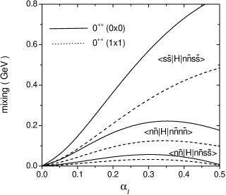
Figure 2: Mixing matrix elements versus $\alpha_{I}$. Solid (dashed) lines are for $q\bar{q}$ spin 0 (1).

For the $0^{++}$ tetra-quark state, the spin of the two $q\bar{q}$ clusters must either be $s_{A}=s_{B}=0~{}{\rm or}~{}s_{A}=s_{B}=1$, and for each the three mixing matrix elements versus $\alpha_{I}$ are shown in Fig. 2. The mixing term is zero when $\alpha_{I}$ is zero and then increases with increasing $\alpha_{I}$. Note that mixing with $s\bar{s}$ states is stronger than with $n\bar{n}$ states.

Using the calculated matrix elements and previously predicted unmixed meson and tetra-quark masses LC2 ; Cotanch ; Ignacio2 , the complete Hamiltonian matrix was diagonalized to obtain the expansion coefficients and masses for the new eigenstates. For $\alpha_{I}=0.2$, the results for $0^{++}$ states are compared in Table 1 to the observed pdg lowest six $0^{++}$ states. Noteworthy, after mixing, the $n\bar{n}$ meson mass is shifted from 848 MeV to 783 MeV and the strange scalar meson mass also decreases from 1297 MeV to 1026 MeV, now close to the experimental value of 980 MeV. Mixing clearly improves the model predictions as the masses of the other $f_{0}$ states are also in better agreement with data. Figure 3 illustrates the over all improved description that mixing provides for the $f_{0}$ spectrum. New structure insight has also been obtained from the coefficients, with the predictions that the $\sigma/f_{0}(600)$ is predominantly a mixture of $n\bar{n}$ and $n\bar{n}n\bar{n}$ states while the $f_{0}(980)$ consists mainly of $s\bar{s}$ and $n\bar{n}s\bar{s}$ states.

Table 1: Mixing coefficients and masses in MeV for isoscalar $0^{++}$ states.

	$|n\bar{n}>$	$|s\bar{s}>$	$|n\bar{n}n\bar{n}>_{1}$	$|n\bar{n}n\bar{n}>_{2}$	$|n\bar{n}s\bar{s}>_{1}$	$|n\bar{n}s\bar{s}>_{2}$
no mixing	848	1297	1282	1418	1582	1718
mixing	783	1026	1295	1466	1611	1962
exp.	$f_{0}(600)$	$f_{0}(980)$	$f_{0}(1370)$	$f_{0}(1500)$	$f_{0}(1710)$	$f_{0}(2020)$
	400 - 1200	$980\pm 10$	1200 - 1500	$1507\pm 5$	$1718\pm 2$	$1992\pm 16$
coeff.	a	b	$c_{1}$	$c_{2}$	$d_{1}$	$d_{2}$
$f_{0}(600)$	0.947	-0.070	0.138	0.277	0.006	0.030
$f_{0}(980)$	0.052	0.838	-0.012	-0.021	0.122	0.529
$f_{0}(1370)$	-0.181	0.026	0.973	0.143	0.002	0.004
$f_{0}(1500)$	-0.248	0.030	-0.187	0.950	0.005	0.009
$f_{0}(1710)$	-0.036	-0.315	0.000	-0.007	0.901	0.295
$f_{0}(2020)$	-0.053	-0.439	0.000	-0.006	-0.416	0.795

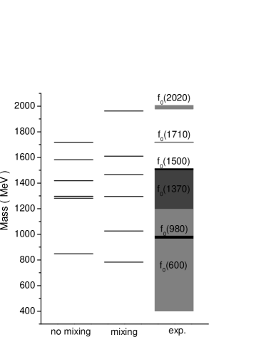
Figure 3: Predicted unmixed, mixed and experimental $f_{0}$ spectrum.

There is general consensus that the $\sigma/f_{0}(600)$ state is a $\pi\pi$ resonance (pole in the $\pi\pi$ scattering amplitude) and thus has a predominantly tetra-quark nature. Because the current numerical treatment of our CG model neglects chiral symmetry, our mass predictions for tetra-quark states which couple to $\pi\pi$ quantum numbers will generally be too heavy and should be regarded as preliminary. A chiral symmetry preserving RPA variational mixing study will be conducted in the future which should yield a lighter scalar tetra-quark mass since our approach is formally equivalent to the Schwinger-Dyson treatment which previously predicted the $\sigma$ is a $\pi\pi$ resonance RPA .

4 Summary and conclusions

Using the established CG model we have calculated $q\bar{q}$ and $q\bar{q}q\bar{q}$ mixing for the low-lying $0^{++}$ spectrum. We find mixing effects are important and necessary for an improved hadronic description. Future work will address mixing applications to glueball and hybrid mesons to facilitate establishing their existence.

References

• (1) F.J. Llanes-Estrada and S.R. Cotanch, Phys. Rev. Lett. 84, 1102 (2000).
• (2) F.J. Llanes-Estrada and S.R. Cotanch, Phys. Lett. B 504, 15 (2001).
• (3) F.J. Llanes-Estrada and S.R. Cotanch, Nucl. Phys. A 697, 303 (2002).
• (4) F.J. Llanes-Estrada, S.R. Cotanch, P. Bicudo, J.E. Ribeiro and A.P. Szczepaniak, Nucl. Phys. A 710, 45 (2002).
• (5) F.J. Llanes-Estrada, P. Bicudo and S.R. Cotanch, Phys. Rev. Lett. 96, 081601 (2006).
• (6) S.R. Cotanch, I.J. General and P. Wang, Eur. Phys. J. A 31, 656 (2007).
• (7) I.J. General, S.R. Cotanch and F.J. Llanes-Estrada, Eur. Phys. J. C 51, 347 (2007).
• (8) I.J. General, P. Wang, S.R. Cotanch and F.J. Llanes-Estrada, Phys. Lett. B 653, 216 (2007).
• (9) W.-M. Yao et al., J. Phys. G 33, 1 (2006).
• (10) P. Bicudo, S.R. Cotanch, F.J. Llanes-Estrada and D.G. Robertson, Eur. Phys. J. C 52, 363 (2007).
• (11) S.R. Cotanch and P. Maris, Phys. Rev. D 66, 116010 (2002); Phys. Rev. D 68, 036006 (2003).