Is the Sun Embedded in a Typical Interstellar Cloud?

Abstract

The physical properties and kinematics of the partially ionized interstellar material (ISM) near the Sun are typical of warm diffuse clouds in the solar vicinity. The direction of the interstellar magnetic field at the heliosphere, the polarization of light from nearby stars, and the kinematics of nearby clouds are naturally explained in terms of the S1 superbubble shell. The interstellar radiation field at the Sun appears to be harder than the field ionizing ambient diffuse gas, which may be a consequence of the low opacity of the tiny cloud surrounding the heliosphere. The spatial context of the Local Bubble is consistent with our location in the Orion spur.

1 Introduction

Observations of interstellar gas in the Milky Way Galaxy span over ten orders-of-magnitude in spatial scales, and over six orders-of-magnitude in temperature. Interstellar material (ISM) is observed at the Earth’s orbit, where interstellar He^o has been counted by the Ulysses GAS detector and is detected through fluorescence of solar 584 A (WellerMeier:1981, ; FlynnVallerga:1998, ; Salernoetal:2003He, ; Witte:2004, ; Moebiusetal:2004, ). Interstellar H^o and other neutral interstellar atoms are driven into the heliosphere by the relative Sun-cloud motion of 26.2 km s^-1, where they become ionized and processed into pickup ions and anomalous cosmic rays. The question arises: ’Is the interstellar cloud feeding gas and dust into the heliosphere a typical interstellar cloud?’ We know more about the circumheliospheric interstellar material (CHISM) than other clouds, because theoretical models combine $in~{}situ$ data with observations of nearby stars to model the cloud opacity profile. In this paper, the kinematics, temperature, ionization, composition and density of the CHISM are compared to low density ISM seen in the solar neighborhood. The answer to the title question is ’yes’.

The properties of the heliosphere are governed by the Local Bubble (LB) void and the Local Interstellar Cloud (LIC). The LB is transparent to radiation, exposing the LIC to a diffuse interstellar radiation field that includes both a soft X-ray background that anticorrelates with the H^o column density (Bowyeretal:1968, ), and radiation from distant hot and white dwarf stars (Gondhalekaretal:1980, ; Vallerga:1998, ). The LIC and ISM surrounding the Sun are part of the shell of a superbubble expanding into the low density interior of the LB. The LIC ionization caused by the radiation field of the hot stars bordering the LB then dominates the heliosphere boundary conditions, while the ram pressure of gas in the expanding superbubble configures the heliosphere into the familiar raindrop shape.

2 Galactic Environment of the Sun

By now it is well known that the Sun resides in a region of space with very low average interstellar densities, the Local Bubble, formed by ISM associated with the ring of young stars bounding this void and known as Gould’s Belt (Frisch:1995, ). The missing part of our understanding has been the origin of the Gould’s Belt stars, or the Orion spur containing these stars. The Orion spur, which is located on the leading edge or convex side of the Sagittarius arm, is not included in models of the Milky Way spiral arms. However recent advances in our understanding of the formation of spurs, or ’feathers’, on spiral arms naturally explains the origin of the Gould’s Belt stars and the Orion spur. The interaction between the gaseous disk and the gravitational potential of spiral arms in the presence of a magnetic field induces self-gravitating perturbations that develop into two-dimensional flows that become unstable and fragment, driving spurs, or ’feathers’, of star-forming material into low-density interarm regions (e.g. (ShettyOstriker:2006, )). The Orion spur can be seen extending between galactic longitude $\ell\sim 60^{\circ}$ distance $\sim 1.2$ kpc, and $\ell\sim 170^{\circ}$ distance $\sim 0.7$ kpc, in Fig. 10 in (Lucke:1978, ), together with two other spurs. These three spurs have pitch angles with respect to a circle around the galactic center of $\sim 40^{\circ}-55^{\circ}$, and are separated by 550–1500 pc, values that are normal for MHD models of spur formation (ShettyOstriker:2006, ). Star formation occurs in spurs, and the Gould’s Belt stars can thus naturally be explained by the Orion spur of which they are part. The Local Bubble is at the inner edge of the Orion spur. Based on MHD models of spur formation, we must conclude that the Gould’s Belt environment of the Sun is normal, answering the question posed above with a ’yes’.

3 Heliospheric ISM

The CHISM ionization balance is governed by photoionization and recombination, so that neutral atoms and dust in the heliosphere trace the cloud physics, as well as the composition, temperature, density, and origin (Slavin and Frisch (SlavinFrisch:2008, )). $In~{}situ$ gas and dust data, combined with radiative transfer models of CHISM ionization, test the ”missing-mass” premise that assumes the combined interstellar atoms in gas and dust provide an invariant tracer of the chemical composition of the ISM (SavageSembach:1996araa, ; Frischetal:1999, ; SlavinFrisch:2008, ). This test is potentially interesting because Gruen and Landgraf (GruenLandgraf:2000, ) have shown that large and small dust grains couple to interstellar gas over different spatial scales, so that in the presence of active or recent grain shattering by interstellar shocks, local and global values for the gas-to-dust mass ratio may differ.

Interstellar particles with gyroradii larger than the distance between the particle and heliopause typically penetrate the heliosphere. If thermal and magnetic pressures are equal in the CHISM, then the magnetic field strength is $\sim 2.7~{}\mu\mathrm{G}$ (Slavin and Frisch (SlavinFrisch:2008, )). Depending on the strength of the radiation field responsible for grain charging through photoejection of electrons, interstellar dust grains entering the heliosphere have radii larger than $\sim 0.06-0.2$ $\mu$m (KruegerGruen:2008, ; Frischetal:1999, ; CzechowskiMann:2003b, ). Grains with radii $\sim 0.01-0.09$ $\mu$m traverse the bow shock region, but are deflected around the heliopause with other charged populations. When STARDUST observations of interstellar grains become available, it will be possible to verify the missing-mass premise that the composition of the CHISM consists of the sum of elements in the gas and dust phases, and check whether solar abundances apply to the CHISM. If the missing-mass assumption is wrong it would explain the $\sim 50$% difference between the gas-to-dust mass ratios found from $in~{}situ$ observations of interstellar grains, and missing mass arguments utilizing radiative transfer models (SlavinFrisch:2008, ).

Only the most abundant interstellar elements with first ionization potentials $\ {\raise-2.15277pt\hbox{$\buildrel>\over{\sim}$}}\ 13.6$ eV are observed in the heliosphere in detectable quantities, including H, He, N, O, Ne, and Ar. Each of these elements is observed in at least two forms, pickup ions (PUI) and anomalous cosmic rays (ACR). ACRs are accelerated PUIs. Pickup ions are formed when interstellar neutrals become ionized through either charge-exchange with the solar wind (H, N, O, Ne, Ar), photoionization (He, H), or electron impact ionization (He, N, Ar). Helium data yield the best temperature, He density, and velocity data, since the He charge-exchange cross-section with the solar wind is low and He penetrates to within $\sim 0.5$ au of the Sun before ionization by photons and electron impact become significant (Moebiusetal:2004, ). The He data indicate for the CHISM: $T=6300\pm 400$ K, $n\mathrm{(He^{\circ})}$=$0.015\pm 0.002$ cm^-3, and $V=-26.2\pm 0.5$ km s^-1, and an upwind direction of $\lambda=255.0^{\circ}\pm 0.6^{\circ}$, $\beta=5.2^{\circ}\pm 0.3^{\circ}$ (corrected for J2000 coordinates, (Moebiusetal:2004, ; Witte:2004, )). Early December each year the Earth passes through a cone of gravitationally focused He, extending over 5 au downwind of the Sun McComasetal:2004Hshadow .

Hydrogen is the most abundant ISM observed in the heliosphere, however the initial thermal interstellar velocity distribution of H^o is modified and deformed as H^o enters and propagates through the heliosphere. Interpretation of the Ly$\alpha$ fluorescence and PUI data require corrections for the weak coupling between H^o and the interstellar magnetic field outside of the heliosphere due to H^o-H⁺ interactions, strong filtration through charge-exchange between interstellar protons and H^o in the heliosheath regions, deformation of the H^o velocity distribution as H atoms enter and propagate through the heliosphere, and the solar-cycle dependent variation in the ratio of radiation pressure and gravitational forces. These effects are discussed elsewhere in this volume (e.g. Bzowski, Quemerais, Wood, Opher, Pogorelov). These observations and models of PUI H inside of the heliosphere are consistent with an H density at the termination shock of $\sim 0.11$ cm^-3, and when combined with filtration values yield an interstellar density of $n(\mathrm{H^{\circ}})\sim 0.195\pm 0.02$ cm^-3 for the CHISM (Bzowskietal:2007, ). The H filtration factor is based on the Moscow Monte Carlo model, which also yields a CHISM plasma density of $n\mathrm{(H^{+})}$$=0.04\pm 0.02$ cm^-3. These results are in excellent agreement with the completely independent radiative transfer results that conclude $n\mathrm{(H^{\circ})}$$=0.19-0.20$ cm^-3, and $n\mathrm{(H^{+})}$$=0.07\pm 0.02$ cm^-3 for the CHISM (SlavinFrisch:2008, ).

Comparisons between abundances of neutrals in the CHISM as predicted by radiative transfer studies, with interstellar neutral abundances based on PUI and ACR densities corrected to values at the termination shock, require that the filtration of neutrals crossing outer heliosheath regions is understood (CummingsStone:2002, ; MuellerZankfilt:2004, ; Izmodenovetal:1999, ). In the heliosheath regions, charge-exchange with interstellar protons increases filtration of O, and reverse charge-exchange potentially allows interstellar O⁺ into the heliosphere. Electron impact ionization contributes to filtration of N and Ar. Reverse charge-exchange between interstellar ions and protons in the outer heliosheath is insignificant for all elements except possibly O and H. The range of filtration factors found for H, He, N, O, Ne, and Ar are listed in (SlavinFrisch:2008, ). Correcting PUI densities given by (GloecklerFisk:2007, ) for the termination shock with calculated filtration factors yields interstellar densities for these elements that are consistent, to within uncertainties, with the range of neutral densities predicted by the CHISM radiative transfer models for these elements (Table 4 in (SlavinFrisch:2008, )). In the radiative transfer models, abundances of H, He, N and O are variables that are required to match the data, but Ne and Ar abundances are assumed at 123 ppm and 2.82 ppm, respectively.

The only measurements of Ne in the local ISM are the $in~{}situ$ PUI and ACR data; Ne is a sensitive tracer of the ionization conditions of the CHISM because three ionization states are present in significant quantities, Ne^∘:Ne⁺:Ne⁺⁺$\sim$1.0:3.3:0.8 (Slavin and Frisch (SlavinFrisch:2008, )). The radiative transfer model results are also consistent with the Ne abundance of $\sim 100$ ppm found in the Orion nebula (Simpson:2004, ), and within the range of uncertainties for the solar Ne abundance.

Neutral Ar traces the equilibrium status of the CHISM because Ar^∘ and H^o are the end products of processes with similar recombination rates, but have different photoionization rates (Slavin, this volume). The radiative transfer models (SlavinFrisch:2008, ) together with the PUI Ar data indicate the CHISM is in ionization equilibrium. The ratio Ar^∘/H^o$\sim 1.0\times 10^{-6}$ in the CHISM found from PUI data and radiative transfer models is comparable to interstellar values towards nearby stars based on the FUV data, Ar^∘/H^o$\sim 1.2\times 10^{-6}$ (Jenkinsetal:2000, ). Agreement with the FUSE data can be achieved by a small increase in the assumed Ar abundances in the (SlavinFrisch:2008, ).

Isotopes in PUIs, ACRs, and He indicate that the CHISM is formed from similar material as the Sun. The ratios ²²Ne/²⁰Ne $\sim 0.073$ and ¹⁸O/¹⁶O $\sim 0.002$ are close to isotopic ratios in the solar wind (CummingsStone:2007, ; Leske:2000, ). He data gives ³He/⁴He $\sim 1.7-2.2\times 10^{-4}$, which is similar to meteoritic and HII region values (Salernoetal:2003He, ; GloecklerFisk:2007, ). Evidently the expected ³He enrichment of the ISM by nucleosynthesis in low-mass stars has not affected the CHISM. The ²²Ne isotope indicates that the CHISM is not significantly mixed with ejecta from Wolf Rayet stars common to OB associations, where ²²Ne would be enriched by He-burning. The CHISM gas therefore appears isotopically similar to solar system material, and ³He values are consistent with isotopic ratios in HII regions.

Summarizing, observations of interstellar products inside of the heliosphere yield densities and abundances for H, He, N, O, Ne, and Ar that are in agreement with radiative transfer models of LIC absorption components in the star $\epsilon$ CMa. Argon has similar abundances, Ar^∘/H^o, in the CHISM and towards near white dwarf stars. Isotopic ratios suggests that the CHISM has a solar composition. $In~{}situ$ observations of interstellar dust grains yield a gas-to-dust mass ratio that varies by 50% or more from values predicted by radiative transfer models, indicating that the either the abundances of elements depleted onto dust grains or the true metallicity of the CHISM is not understood. The CHISM abundances determined from $in~{}situ$ data are consistent with abundances typical of low density ISM, so that based on $in~{}situ$ observations of ISM we conclude that the answer posed above is ’yes’.

4 Kinematics and Temperatures of Very Local ISM versus Warm Interstellar Gas

Using $Copernicus$, IUE, and optical data inside of the heliosphere and towards nearby stars such as $\alpha$ Oph at 14 pc, Frisch (Frisch:1981, ) showed that the ISM inside and close to the heliosphere has the kinematic and abundance properties expected for an origin related to the Loop I superbubble. The first spectrum of Ly$\alpha$ fluorescence from interstellar H^o inside of the heliosphere, acquired by $Copernicus$ during 1975 (AdamsFrisch:1977, ), yielded the H^o velocity in the upwind direction of $\sim-24.7$ km s^-1 (neglecting heliospheric acceleration and converting to the current upstream direction (Witte:2004, ; Frisch:2008S1, )). This H^o velocity projects to $\sim-21.1$ km s^-1 in the $\alpha$ Oph direction, and differs somewhat from the dominant cloud velocities known for that direction of $\sim-24\pm 1$ km s^-1 (MarschallHobbs:1972, ). It is now known that the Ly$\alpha$ line backscattered emission has a significant contribution from secondary H^o atoms, and also that the LIC velocity observed inside of the heliosphere differs by $\sim 1$ km s^-1 from the gas velocity towards the nearest star $\alpha$ Cen, $\sim$50^o from the heliosphere nose (LinskyWood:1996, ), and $\sim 3$ km s^-1 from velocities of nearby gas in the upwind direction towards 36 Oph (Wood36Oph:2000, ). A more complete picture of the kinematics and temperature structure of the LISM is now available. The Sun is embedded in an ISM flow, the complex of local interstellar clouds (CLIC),which has an upwind direction in the Local Standard of Rest (LSR) directed towards the center of the S1 subshell of the Loop I superbubble shell around the Scorpius-Centaurus Association (FrischYork:1986, ; Frisch:1995, ; FGW:2002, ; Wolleben:2007, ; RedfieldLinsky:2008, ). Fig. 1 shows the S1 shell of Wolleben, found by fitting 1.4 GHz and 23 GHz polarization data, the solar apex motion, and the bulk motion of the CLIC through the local standard of rest (LSR). The CLIC LSR upwind direction, $(\ell,b)\sim(358^{\circ},-5^{\circ})$ (FGW:2002, ; FrischSlavin:2006book, ) is $\sim 10^{\circ}$ from the center of the S1 shell at $(\ell,b)\sim(346^{\circ}\pm 5^{\circ},3^{\circ}\pm 5^{\circ})$. The CLIC kinematics is thus naturally explained by the expansion of the S1 shell to the solar location (Frisch:1981, ). The expansion of Loop I has been modeled by Frisch (Frisch:1995, ; Frisch:1996, ), and corresponds to an origin during a star formation epoch $\sim 4-5$ Myrs ago.

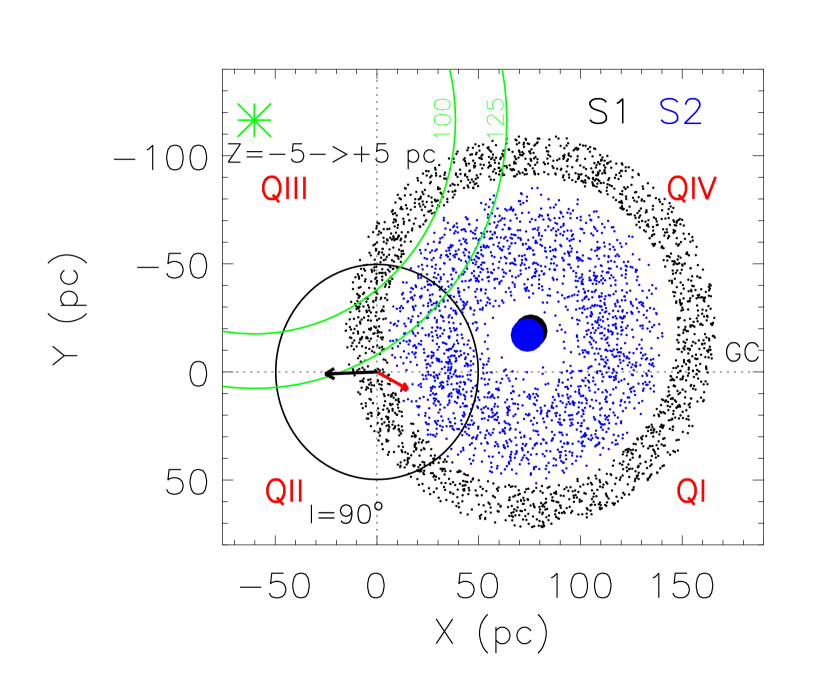
Figure 1: A slice of the S1 (black dots) and S2 (blue dots) shells within 5 pc of the galactic plane ($|$Z$|<5$ pc) are plotted in x,y coordinates, where the x-axis is directed towards the galactic center (from (Frisch:2008S1, )). Red and black arrows show the LSR motions of the Sun and CLIC, respectively. The black circle is 50 pc from the Sun. The two superimposed blue and black large dots show the centers of the two shells. The notation Q1–QIV indicate galactic quadrants. The green star shows the x,y position of the brightest extreme ultraviolet (EUV) source in the sky, $\epsilon$ CMa, which is located 15 pc below the galactic plane. The two concentric green circles show regions 100 pc and 125 pc equidistant from $\epsilon$ CMa. The S1 and S2 shells are constructed using the shell parameters in (Wolleben:2007, ).

Morphologically prominent shells such as the S1 shell are common features in the ISM, often found between spiral arms where spurs are seen. Shell properties have been surveyed in the H^o 21-cm hyperfine transition, revealing filamentary structures consisting partly of warm neutral material (WNM). Column densities for WNM are typically $N$(H^o)$>10^{19}$ cm^-2. WNM with column densities comparable to the CLIC, $N$(H^o)$<10^{18.5}$ cm^-2, or LIC, $N$(H^o)$\sim 10^{17.6}$ cm^-2, are not yet observed. Zeeman data show that shell structures are associated with magnetic fields of $\sim 6.4$ $\mu$G or less. Unfortunately, Zeeman-splitting data show that flux-freezing does not occur in low density ISM, $n<10^{3}$ cm^-3 (CrutcherHT:2003, ), so the magnetic field strength at the solar location can not be inferred from the magnetic field in more distant portions of the S1 shell.

Turning back to the question “Is the Sun embedded in a typical interstellar cloud”. I use the Arecibo Millennium Survey of the H^o 21 cm line to define the meaning of “typical”. The Arecibo survey is a complete and unbiased survey of warm and cold interstellar clouds, as seen from the tropical Arecibo sky (HTI, ). The systematic fitting of Gaussian components to the emission profiles revealed that 60% of the ISM mass is contained in warm neutral material (WNM), with median cloud column densities of $1.3\times 10^{20}$ cm^-2, compared to the lower median column density of the cold neutral medium (CNM) of $5\times 10^{19}$ cm^-2.

The kinematics of the Arecibo clouds can be used as a benchmark for answering the above question as it applies to cloud kinematics. In Fig. 2, left, the kinematics of the CLIC cloudlets (LSR velocities) are compared to the kinematics of the WNM and CNM. For the CLIC velocities I use Ca⁺ and UV absorption line data such as D^o (FGW:2002, ; RLIII, ; Woodetal:2005, ), and for plotting purposes the ratios Ca⁺/H^o$=10^{-8}$ and D^o/H^o$=10^{-4.82}$. It is immediately apparent that the kinematics of CLIC clouds are comparable to the global kinematics of both WNM and CNM clouds in the Arecibo survey.

A second test using the Arecibo is also made. The range of temperatures for the WNM are shown in Fig. 2, right. CLIC temperatures from (RLII, ) are also plotted, although there are still poorly understood aspects of these temperatures (§6). The Arecibo temperatures shown for WNM include both spin temperatures (red arrows) and the kinetic temperatures (red triangles) based on the FWHM of the fitted components. For the WNM, the kinetic and spin temperatures are upper and lower limits on the thermal temperature, respectively, because turbulence is not removed, and the true spin temperature is a function of a limit on the cloud opacity (HTI, ). The median kinetic temperatures for the WNM for clouds for latitudes $b<30^{\circ}$ versus $b>30^{\circ}$ are, respectively, 5,962 K, and 5,182 K. The same ratio of low-to-high latitude WNM temperatures is found for spin temperatures (1.15). Low and high latitude WNM median column densities are, respectively, $N$(H^o)=$10^{20.68}$ cm^-2 and $N$(H^o)$=10^{19.98}$ cm^-2. Since the CHISM temperatures is 6,300 K, it is within the WNM temperature range. Fig. 2, right, shows that the temperatures of the CLIC clouds (green dots) fall consistently between the upper and lower limits on the WNM temperatures. In addition, the CHISM temperature is close to the median kinetic temperature of WNM components with $b<30^{\circ}$. The typical CLIC column densities, $N$(H^o)$<10^{18.5}$ cm^-2, are below the range of detected WNM column densities. Since photoionization dominates the heating of the CHISM (SlavinFrisch:2008, ), the higher low-latitude WNM temperatures also suggest that radiation heating of the ISM is stronger at low latitudes than high latitudes.

Based on the kinematical and temperature information in the Arecibo Millennium Survey, the answer to the question posed above is again ’yes’.

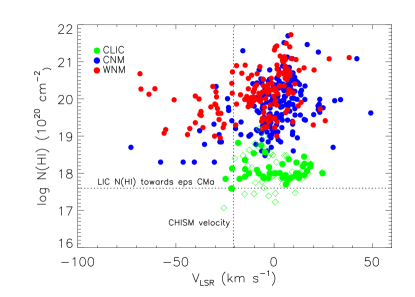
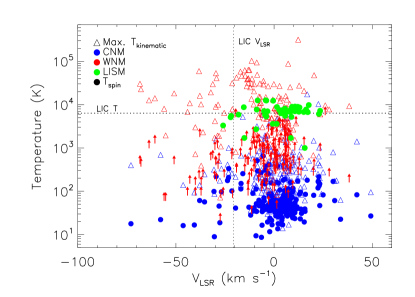
Figure 2: The column densities $N$(H^o), left, and H^o temperatures, right, are plotted as a function of velocity for the WNM (red) and CNM (blue) components in the Arecibo survey (HTI, ) and for the CLIC. The spin temperatures (red arrows) obtained for WNM by (HTI, ) are lower limits. The CLIC components (green dots) are based on Ca⁺ (diamonds, e.g. (FGW:2002, ; Frisch:2008S1, )), H^o, and D^o (dots, (RLIII, ; Woodetal:2005, )). The CHISM LSR velocity is indicated, based on the Standard solar apex motion.

5 Partially Ionized Gas and the Interstellar Radiation Field

Two coupled attributes dominate the CHISM: it is partially ionized, and it is low column density. The first attribute follows from the second in the presence of photons with energies $>13.6$ eV able to ionize H^o. The earliest observations of H^o and He^o inside the solar system found ratios of H^o/He^o$\sim 6$ (Ajelloetal:1987, ; WellerMeier:1981, ), in contrast to EUV observations of five white dwarf stars with average distances of 57 pc and H^o/He^o$\sim 14$ (Frisch:1995, ). Cheng and Bruhweiler (ChengBruhweiler:1990, ) found that hot star radiation dominates H ionization of the LISM but soft X-rays produced He ionization, and therefore yielding higher ionization levels for He compared to H. More recent studies show that He ionization is produced by EUV emission from a conductive interface between the LIC and LB plasma, white dwarf stars, and the low energy tail of the soft X-ray background ((SlavinFrisch:2008, ), Slavin, Shelton, this volume). The low H/He ratio found inside of the heliosphere thus becomes evidence of the strong H filtration in heliosheath regions.

Ionized gas is a major component of the solar neighborhood. FUSE observations of ISM towards white dwarf stars within 70 pc find up to $\sim 70$% ionization levels, and electron densities in the range 0.025–0.25 cm^-3 for stars with $N$(H^o)$=10^{18.8}-10^{19.6}$ cm^-2 (Lehneretal:2003, ). Hydrogen is $\sim 23$% ionized at the heliosphere, which is within the ionization range obtained by FUSE. Radiative transfer models (SlavinFrisch:2008, ) that predict the heliosphere boundary conditions show that the CHISM electron densities of $\sim 0.05-0.09$ cm^-3 are similar to electron densities found by FUSE, and also in the diffuse ionized gas sampled by pulsar dispersion measures and H$\alpha$ recombination lines.

The distribution of ionized gas near the LB is dominated by classic HII regions around hot stars; the Wisconsin H-$\alpha$ Mapper (WHAM) survey of the red H$\alpha$ line shows these regions beautifully (WHAM:2003, ). However, recombination emission from low density ionized gas carries more subtle information about partially ionized regions such as the LIC. Ionized gas in the solar vicinity fills $\sim 20$% of the disk and is contained in warm diffuse low density regions with $n\sim 0.1$ cm^-3 and $T\sim 10^{4}$ K. Ionization of this gas is powered by O-stars, and requires transparent voids through which the O-star radiation can propagate; the Local Bubble is such a void. A detailed comparison of H^o and H$\alpha$ in a $\sim 120$ square-degree of sky showed that at least 30% of the H$\alpha$ emission is both spatially and kinematically associated with warm H^o 21-cm features, many of which are filamentary (ReynoldsTufteHeiles:1995, ). Some of this H⁺ is in regions physically distinct from the H^o gas. Ionization levels reach 40% for these low density, $\sim 0.2-0.3$ cm^-3, clouds. The temperature of diffuse ionized gas varies between 6,000 K and 9,000 K, with higher temperatures at higher latitudes (HaffnerReynoldsTufte:1999, ). This result follows from the temperature dependence of the H$\alpha$ intensity of $\sim T^{-0.9}$, and $[$N⁺$]$ and $[$S⁺$]$ data. The CHISM temperature of 6300 K is within the range for the H$\alpha$ clouds.

Is the diffuse H$\alpha$ emission formed in partially ionized gas similar to the LIC? The answer to this is ’probably’, however whether or not the LIC radiation field is typical of diffuse gas is an open question. Observations of the He^o 5876 A recombination line in the diffuse ionized gas yield low levels of ionized He compared to H, although the dominant O-star ionization source would predict higher levels of He ionization. Reynolds (Reynolds:2004, ) compared LIC radiative transfer model results with the partially ionized LIC gas for four sightlines through diffuse ionized gas where the forbidden 6300 A O^o line is measured. These sightlines indicated H ionization fractions of $>70$%, compared to the LIC value of $\sim 23$%. In addition, for these diffuse gas data, the ionization fraction of He is 30%–60% of that of H, but the absolute He ionization level is similar to the LIC. Together these results suggest that the radiation field at the LIC is harder than the diffuse radiation field that maintains the warm ionized medium. From the relative H and He recombination lines, one thus might conclude that the LIC is not typical of diffuse ionized gas. However, the LIC emission measure is $EM\sim 0.003$ cm^-6 pc, which is below the WHAM sensitivity. Radiative transfer models show that very low column density clouds such as the LIC are transparent to H-ionizing radiation, and such clouds may be invisible to WHAM. The question as to whether the relative ionizations of H and He in the LIC is typical of ionized gas thus remains an open question, but the low LIC column density probably explains the hardness of the local radiation field compared to more distant regions.

Other properties of the interstellar radiation field that are important for LIC ionization include the EUV and soft X-ray fluxes (SlavinFrisch:2008, ). Some doubt has been cast on the absolute flux level of interstellar photons with energies $<0.25$ keV because of contamination of the soft X-ray background (SXRB) by heliospheric emissions at energies $>0.4$ keV from charge-exchange between interstellar neutrals and the solar wind (Shelton, Koutroumpa, this volume). At 0.1 eV, LB emission has been modeled as contributing $\sim 50$% of the flux (HenleyShelton:2007, ). Clumping in the ISM may change this picture, however, since a typical value of $N$(H^o)$\sim 10^{21}$ cm^-2 may include tiny cold clouds such as the $N$(H^o)$\sim 10^{18}$ cm^-2 structures that are completely opaque at low energies (StanimirovicHeiles:2005, ). If the X-ray emitting plasma contains embedded clumps of ISM with significant opacity at $\sim 0.1-0.2$ keV, the energy dependence of the ISM opacity will be significantly altered from that of a homogeneously distributed ISM (KahnJakobsen:1988, ). This effect will be significant for Loop I X-ray emission, where embedded molecular clouds are found. The physical properties of the Local Bubble plasma need to be revisited by including not only foreground emission from charge-exchange between the solar wind and interstellar H^o, but also clumping in the ISM as noted by (KahnJakobsen:1988, ).

There is one point that is not yet appreciated. Since the hot star $\epsilon$ CMa dominates the 13.6 eV radiation field in the solar vicinity, and therefore the flux of H-ionizing photons, sightlines through the third and fourth galactic quadrants (QIII, QIV), $\ell$=180^oto $\ell$=360^o, will sample ISM with higher ionization levels than sightlines through the first two galactic quadrants (Frisch:2008S1, ). This occurs because ISM associated with the S1 shell structure is closer to $\epsilon$ CMa in QIII and QIV, than in the first two galactic quadrants. The relative locations of the S1 shell and $\epsilon$ CMa are shown in Fig. 1.

6 Chemical Composition of the ISM at the Sun

The outstanding feature of warm low density interstellar clouds is that the abundances of refractory elements such as Fe, Ti, and Ca, are enhanced by an order of magnitude when compared to abundances in cold clouds at $\sim 50$ K. The enhanced abundances were originally discovered for the Ca⁺ line seen in high-velocity clouds (RoutlySpitzer:1952, ), although the importance of the ionization balance between Ca⁺⁺ and Ca⁺, which favors Ca⁺⁺ in warm ionized gas, was not fully appreciated at that time. Enhanced abundances are particularly strong for Ti, which is one of the first elements to condense onto dust grains with $T_{\mathrm{condensation}}\sim 1500$ K. Column densities of Ti⁺ can be directly compared with H^o abundances without ionization corrections because Ti⁺ and H^o have similar ionization potentials. Enhanced refractory element abundances in warm gas at higher velocities has been modeled as due to the destruction in shock fronts of refractory-laden interstellar dust grains composed of silicates and/or carbonaceous material (e.g. (Slavinetal:2004, )). The CLIC gas shows such abundances, requiring the CLIC grains to have been processed through shocks of $\sim 80$ km s^-1 (Slavin, this volume, and (Frischetal:1999, )). Refractory elements such as Mg, Si, Fe, and Ca are predominantly singly ionized in the LIC, so that ionization corrections are required to obtain accurate abundance information. Ionization corrections are generally not available for determining abundances of distant warm gas; however the range of uncertainty in elemental abundances is large enough that with or without ionization corrections, the CLIC gas has typical abundances for low density clouds (e.g. (Welty23:1999, )). The radiative transfer models provide accurate CHISM abundances that are discussed by Slavin (this volume), and except for one sightline CHISM abundances are typical for low density ISM.

There is only one sightline through the CLIC that shows a poorly understood abundance pattern, and this is the sightline of $\alpha$ Oph that led to my original conclusion that the Loop I superbubble shell has expanded to the solar location (Frisch:1981, ). The strongest observed Ca⁺ line in the CLIC is towards $\alpha$ Oph, where strong Ti⁺ is also seen. The star $\alpha$ Oph is 14 pc from the Sun in the direction of the North Polar Spur, and the interstellar gas in this sightline may be in the region where the S1 and S2 shells are in collision, so that shock destruction of the grains is underway.

Two caveats must be attached to most determinations of elemental abundances: (1) Common refractory elements tend to have FIP’s $<13.6$ eV, so that ionization corrections are required to obtain accurate abundances. (2) Accurate H^o column densities are also required so that abundances per H-atom can be calculated. The first requirement is seldom met, because cloud ionization data at best typically return electron densities calculated based on either Mg^o/Mg⁺ or C^+∗/C⁺⁺ ratios. Total H⁺ column densities are not directly measured and must be inferred. Optimally, radiative transfer models of each cloud could provide the same quality of results now available for the LIC. The second requirement is notoriously difficult to achieve for H^o values relying on the heavily saturated Ly$\alpha$ line.

There are difficulties with extracting reliable column densities from lines where thermal line-broadening dominates turbulent line-broadening. The Voigt profile used to determine the parameters of absorption lines invokes the Doppler b-value ($b_{\mathrm{D}}\sim FWHM/1.7$):

$$b_{\mathrm{D}}(T,m)^{2}=b_{\mathrm{thermal}}(T,m)^{2}+b_{\mathrm{turbulent}}^{2},$$ (1)

where $b_{\mathrm{turbulent}}$ has no mass ($m$) or temperature ($T$) dependence. This assumption appears to break down for stars within 10 pc of the Sun, as is shown in Fig. 3 (using data from (RLIII, )) by the correlation between $N$(D^o) and temperature $T$, and the anticorrelation between $b_{\mathrm{thermal}}(T,2)$ and turbulence $\xi=b_{\mathrm{turbulent}}$. No known cloud physics explains a correlation between D^o and $T$ that is accompanied by an anticorrelation between turbulent and thermal broadening. One explanation for this effect is that the assumption of isotropic Maxwellian gas velocities and mass-independent turbulence breaks down in a partially ionized low density ISM due to the coupling between ions and magnetic fields.

Figure 3: Temperature versus column density $N$(DI) (left ) and temperature versus turbulence $\xi$ (right) for interstellar absorption components seen towards stars within 10 pc of the Sun (data from (RLIII, )).

The summary conclusion of this section is that CLIC and CHISM abundances are similar to abundances in partially ionized gas. Because of the uncertainties, this statement holds true when elemental abundances are correctly compared to H^o+H⁺, or H^o alone. The one caveat on this statement is that D^o column densities for stars within 10 pc show evidence of correlations that indicate the line-broadening parameter is incorrectly defined. The one sightline that is not typical is $\alpha$ Oph, which may hold hidden clues about colliding superbubbles near the Sun.

7 Interstellar Magnetic Field at the Solar Location

The orientation, but not the polarity, of the interstellar magnetic field (ISMF) at or near the heliosphere can be derived from optical polarization vectors for nearby stars, $<30$ pc. This orientation can then be compared with the local magnetic field direction derived from the S1 shell low frequency radio continuum polarization (1.4 GHz, Wolleben (Wolleben:2007, ), Frisch (Frisch:2008S1, )). The strongest optical polarizations are seen for stars located along the ecliptic plane and with a peak in the polarization that is offset by $\lambda\sim 40^{\circ}$ from the direction of the heliosphere nose (Frisch:2008S1, ). The orientation of the S1 shell magnetic field in the heliosphere nose region agrees with the values obtained from the optical polarization direction, to within the uncertainties, for the Wolleben (Wolleben:2007, ) angle parameter $B_{\phi}=-42^{\circ}$. The magnetic field at the position of the polarized stars forms an angle of $\sim 65^{\circ}\pm 9^{\circ}$ with respect to the ecliptic plane, and $\sim 55^{\circ}\pm 9^{\circ}$ with respect to the galactic plane. At the position of the He^o inflow direction, the S1 shell configuration consistent with the polarization data gives a magnetic field inclination of $\sim 73^{\circ}\pm 10^{\circ}$ with respect to the ecliptic plane, and $\sim 44^{\circ}\pm 10^{\circ}$ with respect to the galactic plane. When the uncertainties on the upwind directions of interstellar H^o and He^o flowing into the heliosphere are considered, then the offset angle between these two inflow directions is $4.8^{\circ}\pm 0.6^{\circ}$, and these two upwind directions define an angle of $55^{\circ}\pm 20^{\circ}$ with respect to an ecliptic parallel (Frisch:2008S1, ; Moebiusetal:2004, ; Lallementetal:2005, ). When the uncertainties are considered the H^o–He^o offset angle, and the S1 shell direction that is consistent with the optical polarization data, yield consistent ISMF orientations.

A non-zero angle between the ISMF direction and the inflowing ISM velocity vector causes an asymmetric heliosphere, including a possible tilt of $\sim 12^{\circ}$ between the heliosphere nose, as defined by the maximum outer heliosheath plasma density, and the ISM velocity (e.g. (Ratkiewiczetal:1998, ; Lindeetal:1998, ; Ratkiewiczetal:2008, )). Is the S1 shell field orientation at the heliosphere consistent with models of the known asymmetries of the heliosphere? Pogorelov et al. (PogorelovOgino:2008, ) argue that large angles between the upwind ISM and magnetic field directions are required to reproduce the heliospheric asymmetry seen by the Voyager 1 and Voyager 2, which encountered different termination shock distances at $\sim 94$ au and $\sim 84$ au (Stone:2008, ). A magnetic field direction tilted by $\sim 60^{\circ}$ with respect to the ecliptic plane reproduces the offset angle between H^o-He^o, but not the heliospheric asymmetry seen by the Voyager satellites (Pogorelov et al. (PogorelovOgino:2008, )). Opher (Opher:2008, ) reports that an interstellar field direction inclined by $\sim 60^{\circ}-90^{\circ}$ with respect to the galactic plane reproduces the Voyager results, including particle streaming in the outer heliosheath. Ratkiewicz et al. (Ratkiewiczetal:2008, ) find that an ISMF directed towards galactic coordinates $\ell$$=217^{\circ}\pm 14^{\circ}$, $b$$=-50^{\circ}\pm 9^{\circ}$ explains the position of the Ly$\alpha$ maximum observed by the Voyager spacecraft in the outer heliosphere. These models, the interstellar polarization data, and the S1 shell predictions of the ISMF direction at the heliosphere agree to within the large uncertainties remaining in this problem.

If magnetic and thermal pressures in the CHISM are approximately equal, then the CHISM field strength is $\sim 2.7$ $\mu$G (SlavinFrisch:2008, ). The polarity of the CHISM field is a more difficult question, and can presently only be inferred from the polarity of the nearby global magnetic field. The global magnetic field direction in the solar vicinity is directed towards $\ell$$\sim 80^{\circ}$ (Han:2006, ). For a classical expanding superbubble model (MacLowMcCray:1988, ), where a shock front sweeps up interstellar material and compresses magnetic field lines in the expanding shell, the S1 shell expansion would have preserved the global field polarity so that the S1 shell field direction at the Sun is directed from the south to north. With this polarity, the direction of the interstellar magnetic field at the heliosphere nose is shown in Fig. 4 (see (Frisch:2008S1, ) for the field direction in galactic coordinates). This model neglects possible additional rotation of the field direction, such as may arise from coupling between the ISMF and $\sim 18^{\circ}$ tilt of the plane of Goulds Belt with respect to the galactic plane.

Based on the similar magnetic field directions obtained from the S1 shell magnetic field at the heliosphere and the polarization of light for stars close to the Sun, the magnetic field in the CLIC and CHISM is typical. The field strength inferred from pressure equilibrium in the CHISM, $\sim 2.7$ $\mu$G, is typical of field strengths found from Zeeman splitting of the 21-cm line for WNM in the Arecibo survey, and $\sim 50$% larger than the large-scale ordered magnetic component inferred from pulsar data (RandKulkarni:1989, ). Given that there is no evidence that the interstellar magnetic field at the heliosphere is anomalous, again the answer to the posed question is ’yes’.

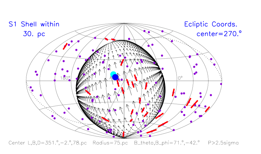
Figure 4: The magnetic field associated with the parts of the S1 shell within 30 pc is plotted in ecliptic coordinates for an aitoff projection. The parameters for the S1 shell given in (Wolleben:2007, ) have been varied within the range of allowed uncertainties to yield the best match to polarization data towards stars in the heliosphere nose region (indicated by the dark blue dots). The dark and light blue dots show the inflow directions of interstellar He^o and H^o into the heliosphere. The S1 subshell parameters used in the above figures correspond to a shell center at ($\ell$,$b$)=$(351^{\circ},-2^{\circ})$ and a distance of 78 pc away, a shell radius of 75 pc, and magnetic field angles $B_{\theta}=71^{\circ}$ and $B_{\phi}=-42^{\circ}$. The dots show stars within 50 pc with polarization data, and the red bars show polarization vectors for stars where polarizations are larger than $2.5\sigma$ (Tinbergen:1982, ; Piirola:1977, ; Frisch:2007cmb, ).

8 Conclusions

By all of the standard measures of interstellar clouds, such as temperature, velocity, composition, ionization, and magnetic field, the interstellar gas inside of the heliosphere and in the LIC are typical of warm partially ionized gas seen elsewhere in the neighborhood of the Sun. Unfortunately clouds with low LIC-like column densities are not yet observable in either H^o 21-cm or H$\alpha$ recombination lines, so that clouds with hard radiation fields similar to the LIC can only be idenitified through ultraviolet absorption lines.

The association of the LISM and LIC gas with the expanding S1 supersubble shell, and possibly the S2 shell, naturally explains the kinematics of ISM within $\sim 30$ pc. Furthermore, the S1 shell structure leads to specific predictions about the relative ionizations of different parts of the shell due to proximity to $\epsilon$ CMa and other nearby hot stars (FrischChoi:2008, ). The S1 shell also predicts a direction of the interstellar magnetic field at the heliosphere that is consistent with observations of optical polarizations towards nearby stars.

It is evident that the answer to the question posed by the title of this paper is ’yes’, so this paper will close with a more difficult question posed years ago by Eugene Parker: ”What is an interstellar cloud”. Originally clouds like the LIC and other LISM clouds were named ”intercloud medium”. The LIC column density towards Sirius, $\alpha$ CMa, suggests the Sun has entered the LIC within the past few thousand years (Frisch (Frisch:1994, )), while the velocity discrepancy between interstellar He^o inside of the heliosphere and ISM in the upwind direction towards $\alpha$ Cen and 36 Oph suggests the Sun is at the edge of the LIC (Lallement et al. (Lallementetal:1995, ), Wood et al. (Wood36Oph:2000, )). Are there two separate clouds adjacent to the heliosphere? Or instead are we crossing a pocket of microturbulence with scale sizes of $\sim 0.02$ pc? What is a cloud anyway? The LIC is $\sim 10^{21}$ orders-of-magnitude less dense than the terrestrial atmosphere.

- [1] T. F. Adams and P. C. Frisch. High-resolution observations of the Lyman alpha sky background. ApJ, 212:300–308, 1977.
- [2] J. M. Ajello, A. I. Stewart, G. E. Thomas, and A. Graps. Solar cycle study of interplanetary Lyman-alpha variations - Pioneer Venus Orbiter sky background results. ApJ, 317:964–986, June 1987.
- [3] C. S. Bowyer, G. B. Field, and J. F. Mack. Detection of an Anisotropic Soft X-Ray Background Flux. Nature, 217:32–+, January 1968.
- [4] M. Bzowski, E. Moebius, S. Tarnopolski, V. Izmodenov, and G. Gloeckler. Density of neutral interstellar hydrogen at the termination shock from Ulysses pickup ion observations. ArXiv e-prints, 710, 2007.
- [5] K. Cheng and F. C. Bruhweiler. Ionization processes in the local interstellar medium - Effects of the hot coronal substrate. ApJ, 364:573–581, 1990.
- [6] R. Crutcher, C. Heiles, and T. Troland. Observations of Interstellar Magnetic Fields. Lecture Notes in Physics, Berlin Springer Verlag, 614:155–181, 2003.
- [7] A. C. Cummings and E. C. Stone. Composition of Anomalous Cosmic Rays. Space Science Reviews, 130:389–399, 2007.
- [8] A. C. Cummings, E. C. Stone, and C. D. Steenberg. Composition of Anomalous Cosmic Rays and Other Heliospheric Ions. ApJ, 578:194–210, 2002.
- [9] A. Czechowski and I. Mann. Local interstellar cloud grains outside the heliopause. A&A, 410:165–173, 2003.
- [10] B. Flynn, J. Vallerga, F. Dalaudier, and G. R. Gladstone. EUVE detection ofthe local interstellar wind and geocorona via resonance scattering of solar HeI 584 A line emission. J. Geophys. Res., 103:6483, 1998.
- [11] P. Frisch and D. G. York. Interstellar clouds near the Sun. In The Galaxy and the Solar System, pages 83–100. University of Arizona Press, 1986.
- [12] P. C. Frisch. The nearby interstellar medium. Nature, 293:377–379, 1981.
- [13] P. C. Frisch. Morphology and ionization of the interstellar cloud surrounding the solar system. Science, 265:1423, 1994.
- [14] P. C. Frisch. Characteristics of nearby interstellar matter. Space Sci. Rev., 72:499–592, 1995.
- [15] P. C. Frisch. LISM Structure - Fragmented superbubble shell? Space Sci. Rev., 78:213–222, 1996.
- [16] P. C. Frisch. Implications of Interstellar Dust and Magnetic Field at the Heliosphere. ArXiv e-prints, 707, 2007.
- [17] P. C. Frisch. The S1 Shell and Interstellar Magnetic Field and Gas near the Heliosphere. ApJ, ’submitted’, 2008.
- [18] P. C. Frisch, A. Choi, D. G. York, and L. M. Hobbs. Observations of CaII and NaI in the Local Interstellar Medium. in preparation, 000:000, 2008.
- [19] P. C. Frisch, J. M. Dorschner, J. Geiss, J. M. Greenberg, E. Grün, M. Landgraf, P. Hoppe, A. P. Jones, W. Krätschmer, T. J. Linde, G. E. Morfill, W. Reach, J. D. Slavin, J. Svestka, A. N. Witt, and G. P. Zank. Dust in the Local Interstellar Wind. ApJ, 525:492–516, 1999.
- [20] P. C. Frisch, L. Grodnicki, and D. E. Welty. The Velocity Distribution of the Nearest Interstellar Gas. ApJ, 574:834–846, 2002.
- [21] P. C. Frisch and J. D. Slavin. Short Term Variations in the Galactic Environment of the Sun, in Solar Journey: The Significance of Our Galactic Environment for the Heliosphere and Earth, Ed. P. C. Frisch. 2006.
- [22] G. Gloeckler and L. Fisk. Johannes Geiss’ Investigations of Solar, Heliospheric and Interstellar Matter. “Composition of Matter”, Space Sciences Series of ISSI, publ. Springer, 27:00, 2007.
- [23] P. M. Gondhalekar, A. P. Phillips, and R. Wilson. Observations of the interstellar ultraviolet radiation field from the s2/68 sky-survey telescope. A&A, 85:272, May 1980.
- [24] E. Gruen and M. Landgraf. Collisional consequences of big interstellar grains. J. Geophys. Res., 105:10291–10298, 2000.
- [25] L. M. Haffner, R. J. Reynolds, and S. L. Tufte. WHAM Observations of Halpha, [S II], and [N II] toward the Orion and Perseus Arms: Probing the Physical Conditions of the Warm Ionized Medium. ApJ, 523:223–233, 1999.
- [26] L. M. Haffner, R. J. Reynolds, S. L. Tufte, G. J. Madsen, K. P. Jaehnig, and J. W. Percival. The Wisconsin H Mapper Northern Sky Survey. ApJS, 149:405–422, 2003.
- [27] J. L. Han. Magnetic Fields in Our Galaxy: How much do we know? III. Progress in the Last Decade. Chinese Journal of Astronomy and Astrophysics Supplement, 6:211–217, 2006.
- [28] C. Heiles and T. H. Troland. The Millennium Arecibo 21 Centimeter Absorption-Line Survey. I. Techniques and Gaussian Fits. ApJS, 145:329–354, 2003.
- [29] D. B. Henley, R. L. Shelton, and K. D. Kuntz. An XMM-Newton Observation of the Local Bubble Using a Shadowing Filament in the Southern Galactic Hemisphere. ArXiv Astrophysics e-prints, 2007.
- [30] V. V. Izmodenov, J. Geiss, R. Lallement, G. Gloeckler, V. B. Baranov, and Y. G. Malama. Filtration of interstellar hydrogen in the two-shock heliospheric interface: Inferences on the local interstellar cloud electron density. J. Geophys. Res., 104:4731–4742, 1999.
- [31] E. B. Jenkins, W. R. Oegerle, C. Gry, J. Vallerga, K. R. Sembach, R. L. Shelton, R. Ferlet, A. Vidal-Madjar, D. G. York, J. L. Linsky, K. C. Roth, A. K. Dupree, and J. Edelstein. The Ionization of the Local Interstellar Medium as Revealed by Far Ultraviolet Spectroscopic Explorer Observations of N, O, and AR toward White Dwarf Stars. ApJ, 538:L81–L85, July 2000.
- [32] S. M. Kahn and P. Jakobsen. On the interpretation of the soft X-ray background. II - What do the beryllium band data really tell us? ApJ, 329:406–409, 1988.
- [33] H. Krueger and E. Gruen. Interstellar Dust Inside and Outside the Heliosphere. ArXiv e-prints, 802, 2008.
- [34] R. Lallement, R. Ferlet, A. M. Lagrange, M. Lemoine, and A. Vidal-Madjar. Local cloud structure from HST-GHRS. A&A, 304:461–474, 1995.
- [35] R. Lallement, E. Quémerais, J. L. Bertaux, S. Ferron, D. Koutroumpa, and R. Pellinen. Deflection of the Interstellar Neutral Hydrogen Flow Across the Heliospheric Interface. Science, 307:1447–1449, March 2005.
- [36] N. Lehner, E. Jenkins, C. Gry, H. Moos, P. Chayer, and S. Lacour. FUSE Survey of Local Interstellar Medium within 200 Parsecs. ApJ, 595:858–879, 2003.
- [37] R. A. Leske. Anomalous Cosmic Ray Composition from ACE. In B. L. Dingus, D. B. Kieda, and M. H. Salamon, editors, AIP Conf. Proc. 516: 26th International Cosmic Ray Conference, ICRC XXVI, pages 274–+, 2000.
- [38] T. J. Linde, T. I. Gombosi, P. L Roe, K. G. Powell, and D. L. DeZeeuw. Heliosphere in the magnetized local interstellar medium: Results of a three-dimensional MHD simulation. J. Geophys. Res., 103:1889–1904, 1998.
- [39] J. L. Linsky and B. E. Wood. The alpha Centauri line of sight: D/H ratio, physical properties of local interstellar gas, and measurement of heated hydrogen (the ‘hydrogen wall’) near the heliopause. ApJ, 463:254–270, 1996.
- [40] P. B. Lucke. The distribution of color excesses and interstellar reddening material in the solar neighborhood. A&A, 64:367–377, 1978.
- [41] E. Möbius, M. Bzowski, S. Chalov, H.-J. Fahr, G. Gloeckler, V. Izmodenov, R. Kallenbach, R. Lallement, D. McMullin, H. Noda, M. Oka, A. Pauluhn, J. Raymond, D. Ruciński, R. Skoug, T. Terasawa, W. Thompson, J. Vallerga, R. von Steiger, and M. Witte. Synopsis of the Interstellar He Parameters from Combined Neutral Gas, Pickup Ion and UV Scattering Observations. A&A, 426:897–907, 2004.
- [42] H.-R. Müller and G. P. Zank. Heliospheric filtration of interstellar heavy atoms: Sensitivity to hydrogen background. J. Geophys. Res., pages 7104–7116, 2004.
- [43] M. MacLow and R. McCray. Superbubbles in disk galaxies. ApJ, 324:776–785, 1988.
- [44] L. A. Marschall and L. M. Hobbs. Interferometric Studies of Interstellar Calcium Lines. ApJ, 173:43–62, 1972.
- [45] D. J. McComas, N. A. Schwadron, F. J. Crary, H. A. Elliott, D. T. Young, J. T. Gosling, M. F. Thomsen, E. Sittler, J.-J. Berthelier, K. Szego, and A. J. Coates. The interstellar hydrogen shadow: Observations of interstellar pickup ions beyond Jupiter. Journal of Geophysical Research (Space Physics), 109:2104–+, 2004.
- [46] M. Opher. Role of the Interstellar Magnetic Field in the Flows in the Heliosheath. AGU-Spring Meeting, Florida, pages Paper SH24A–08, 2008.
- [47] V. Piirola. Polarization observations of 77 stars within 25 PC from the Sun. A&AS, 30:213–+, November 1977.
- [48] N. V. Pogorelov, G. P. Zank, and T. Ogino. MHD modeling of the outer heliosphere: Achievements and challenges. Advances in Space Research, 41:306–317, 2008.
- [49] R. J. Rand and S. R. Kulkarni. The local Galactic magnetic field. ApJ, 343:760–772, 1989.
- [50] R. Ratkiewicz, A. Barnes, G. A. Molvik, J. R. Spreiter, S. S. Stahara, M. Vinokur, and S. Venkateswaran. Effect of varying strength and orientation of local interstellar magnetic field on configuration of exterior heliosphere: 3D MHD simulations. A&A, 335:363–369, 1998.
- [51] R. Ratkiewicz, L. Ben-Jaffel, and J. Grygorczuk. What Do We Know about the Orientation of the Local Interstellar Magnetic Field? In N. V. Pogorelov, E. Audit, and G. P. Zank, editors, Numerical Modeling of Space Plasma Flows, volume 385 of Astronomical Society of the Pacific Conference Series, page 189, 2008.
- [52] S. Redfield and J. L. Linsky. The Structure of the Local Interstellar Medium. II. Observations of D I, C II, N I, O I, Al II, and Si II toward Stars within 100 Parsecs. ApJ, 602:776–802, 2004.
- [53] S. Redfield and J. L. Linsky. The Structure of the Local Interstellar Medium. III. Temperature and Turbulence. ApJ, 613:1004–1022, 2004.
- [54] S. Redfield and J. L. Linsky. The Structure of the Local Interstellar Medium. IV. Dynamics, Morphology, Physical Properties, and Implications of Cloud-Cloud Interactions. ApJ, 673:283–314, 2008.
- [55] R. J. Reynolds. Warm ionized gas in the local interstellar medium. Advances in Space Research, 34:27–34, 2004.
- [56] R. J. Reynolds, S. L. Tufte, D. T. Kung, P. R. McCullough, and C. Heiles. A Comparison of Diffuse Ionized and Neutral Hydrogen Away from the Galactic Plane: H alpha -emitting H I Clouds. ApJ, 448:715–726, 1995.
- [57] P. Routly and Jr. Spitzer, L. A comparison of the components in interstellar sodium and calcium. ApJ, 115:227, 1952.
- [58] E. Salerno, F. Bühler, P. Bochsler, H. Busemann, M. L. Bassi, G. N. Zastenker, Y. N. Agafonov, and N. A. Eismont. Measurement of 3He/4He in the Local Interstellar Medium: the Collisa Experiment on Mir. ApJ, 585:840–849, 2003.
- [59] B. D. Savage and K. R. Sembach. Interstellar abundances from absorption-line observations with the Hubble Space Telescope. ARA&A, 34:279–330, 1996.
- [60] R. Shetty and E. C. Ostriker. Global Modeling of Spur Formation in Spiral Galaxies. ApJ, 647:997–1017, 2006.
- [61] J. P. Simpson, R. H. Rubin, S. W. J. Colgan, E. F. Erickson, and M. R. Haas. On the Measurement of Elemental Abundance Ratios in Inner Galaxy H II Regions. ApJ, 611:338–352, 2004.
- [62] J. D. Slavin and P. C. Frisch. The Boundary Conditions of the Heliosphere: Photoionization Models Constrained by Interstellar and In Situ Data. A&A, in press, 000:0000–0000, 2008.
- [63] J. D. Slavin, A. P. Jones, and A. G. G. M. Tielens. Shock Processing of Large Grains in the Interstellar Medium. ApJ, 614:796–806, October 2004.
- [64] S. Stanimirovic and C. Heiles. The thinnest cold HI clouds in the diffuse interstellar medium? ArXiv Astrophysics e-prints, May 2005.
- [65] E. Stone. Voyager 2 Observations of the Solar Wind Termination Shock and Heliosheath. AGU-Spring Meeting, Florida, pages Paper SH24A–01, 2008.
- [66] J. Tinbergen. Interstellar polarization in the immediate solar neighborhood. A&A, 105:53–64, 1982.
- [67] John Vallerga. The stellar extreme-ultraviolet radiation field. ApJ, 497:921–927, 1998.
- [68] C. S. Weller and R. R. Meier. Characteristics of the helium component of the local interstellar medium. ApJ, 246:386–393, 1981.
- [69] D. E. Welty, L. M. Hobbs, J. T. Lauroesch, D. C. Morton, L. Spitzer, and D. G. York. The diffuse interstellar clouds toward 23 Orionis. ApJS, 124:465–501, 1999.
- [70] M. Witte. Kinetic parameters of interstellar neutral helium. Review of results obtained during one solar cycle with the Ulysses/GAS-instrument. A&A, 426:835–844, 2004.
- [71] M. Wolleben. A New Model for the Loop I (North Polar Spur) Region. ApJ, 664:349–356, 2007.
- [72] B. E. Wood, J. L. Linsky, and G. P. Zank. Heliospheric, astrospheric, and interstellar ly-alpha; absorption toward 36 Ophiuchi. ApJ, 537:304–311, 2000.
- [73] B. E. Wood, S. Redfield, J. L. Linsky, H.-R. Müller, and G. P. Zank. Stellar Ly Emission Lines in the Hubble Space Telescope Archive: Intrinsic Line Fluxes and Absorption from the Heliosphere and Astrospheres. ApJS, 159:118–140, 2005.