Dynamics of saturated Bragg diffraction in a stored light grating in cold atoms

Abstract

We report on a detailed investigation of the dynamics and the saturation of a light grating stored in a sample of cold cesium atoms. We employ Bragg diffraction to retrieve the stored optical information impressed into the atomic coherence by the incident light fields. The diffracted efficiency is studied as a function of the intensities of both writing and reading laser beams. A theoretical model is developed to predict the temporal pulse shape of the retrieved signal and compares reasonably well with the observed results.

I Introduction

The storage of light information in an atomic ensemble is a well understood phenomenon which has a promising prospect for application both in classical and quantum information processing Lukin03 . The light storage (LS) phenomenon allows us to obtain later information on a previously stored light pulse, as well as to manipulate the stored information. As it was first proposed, LS in an electromagnetically induced transparency (EIT) medium Harris97 ; Fleischhauer05 is described in terms of a mixed two component light-matter excitation, called dark state polariton (DSP), where each component of the excitation can be externally controlled Freischhauer00 . To date, several experimental observations of these effects were realized in different systems Phillips01 ; Liu01 ; Zibrov02 ; Mair02 ; Wang05 .

Alternatively, the LS process can also be described as being due to the creation of a spatially dependent ground states coherence that contains respectively the information on the amplitude and phase of a light pulse and which survives after the switching-off of the incident light. Using this simpler picture, we have recently demonstrated the storage of a polarization light grating into an atomic coherence via a backward four-wave mixing configuration Tabosa07 . Others schemes have also been recently employed to store spatial structures (images) in atomic vapors Shuker07 ; Pugatch07 . For instance, a light vortex was stored in a hot vapor for hundreds of microseconds Pugatch07 .

In this work we present experimental and theoretical investigation on the dynamics of light grating stored in an EIT medium associated with a degenerate two-level system. The dependence of the stored light grating with the intensities of the incident writing and reading beams is investigated. Bragg diffraction into the stored grating is employed to probe its dynamics under different experimental conditions. The demonstration of the reversible storage and the manipulation of the spatial light phase structure stored into the atomic ensemble, and its extension to include beams carrying orbital angular momentum, would be of great importance to demonstrate the manipulation of quantum information encoded in a higher dimensional state space Padgett04 ; Barreiro03 . Moreover, the storage of this light grating opens up the possibility to investigate the generation of correlated photons pairs in a previously coherently prepared atomic ensemble Balic05 .

II Theoretical model

We consider an ensemble of cold atoms excited by three different fields: two writing ($W$ and $W^{\prime}$) and one reading ($R$) laser pulses. The atomic ensemble can be well approximated by a set of degenerate two-level atoms, with a ground-state manifold composed of two degenerate states ($|1a\rangle$ and $|1b\rangle$) and the excited-state manifold having a single state ($|2\rangle$). As illustrated in Fig. 1, the ground-state degeneracy corresponds to the Zeemam degeneracy of atomic cesium in the experiment. In this way, the different levels are connected by fields of different polarizations with respect to the atom. We consider fields $W^{\prime}$ and $R$ having $\hat{\sigma}^{-}$ polarization and field $W$ having $\hat{\sigma}^{+}$ polarization. $W^{\prime}$ and $R$ excite then the transition $1b\rightarrow 2$, and $W$ the transition $1a\rightarrow 2$.

The fields $W$ and $W^{\prime}$ propagate in different directions, corresponding to a small angle $\theta$ between them. The $R$ field is counter-propagating with respect to $W$. The signal we want to model corresponds to the diffraction of the $R$ field in the spatial grating formed by fields $W$ and $W^{\prime}$. In the case of cw excitation of the ensemble, this signal corresponds to the well-know conjugated signal in four-wave mixing (FWM) processes Lezama01 . Here we call it $D$ field (see Fig. 1b).

We use this FWM configuration to store and later retrieve a coherence grating written in the atomic ensemble. In order to address this coherence storage process, we use a specific time sequence for the pulsed excitation of the ensemble, see Fig. 1c. First we prepare the sample by exciting it with the two, long writing pulses. In this writing process, the goal is to leave the system in its stationary state. Then we turn off the writing beams, and wait a certain amount of time, the storage time, before turning the reading pulse on. This reading pulse stays on also for a long time, enough to extract the whole stored grating from the ensemble. A field-$D$ pulse is then generated during the read process. In the following theoretical analysis, we want to model and study this field-$D$ generation process in detail, considering the three-level-atom approximation discussed above.

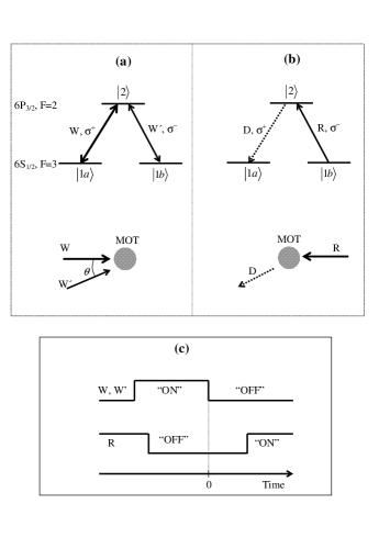
Figure 1: (a) Simplified Zeeman level scheme, showing the coupling and the propagation directions of the grating writing beams ($W$ and $W^{\prime}$) and (b) the coupling and the propagation direction of the reading ($R$) and diffracted ($D$) beams. The beams $W$ and $W^{\prime}$ make a small angle $\theta$ and are circularly polarized with opposite handedness, while the beam $R$ is counterpropagating to the beam $W$ and have a circular polarization opposite to this beam. The diffracted beam is detected in a direction opposite to the beam $W^{\prime}$.(c) The switching time sequence for the writing and reading beams.

II.1 Grating formation and storage

Consider an atom excited by two writing beams: one, $\vec{E}_{W}$, propagating in the $z$ direction and the other, $\vec{E}_{W^{\prime}}$, forming an angle $\theta$ with $\vec{E}_{W}$. The fields $\vec{E}_{W}$ and $\vec{E}_{W^{\prime}}$ have orthogonal circular polarizations $\hat{\sigma}^{+}$ and $\hat{\sigma}^{-}$, respectively. We consider small enough angles so that we can assume, to a good approximation, the polarization of $\vec{E}_{W^{\prime}}$ as being $\hat{\sigma}^{-}$ on the same state basis in which $\vec{E}_{W}$ is $\hat{\sigma}^{+}$. We can then write

$$\vec{E}_{W} ={\cal E}_{W}(\vec{r})e^{i(k_{W}z-\omega_{W}t)}\hat{\sigma}^{+}\;,$$ (1a)

$$\vec{E}_{W^{\prime}} ={\cal E}_{W^{\prime}}(\vec{r})e^{i(\vec{k}_{W^{\prime}}\cdot\vec{r}-\omega_{W^{\prime}}t)}\hat{\sigma}^{-}\;,$$ (1b)

where ${\cal E}_{W}(\vec{r})$ and ${\cal E}_{W^{\prime}}(\vec{r})$ represent the transversal modes of each field, and we assumed both of them having constant intensities. The frequencies of the fields are $\omega_{W}$ and $\omega_{W^{\prime}}$, and their wavevectors are $k_{W}\hat{z}$ and $\vec{k}_{W^{\prime}}$, respectively. The energy difference between fundamental and excited levels is $\hbar\omega_{e}$.

The system hamiltonian can then be written as

$$\hat{H}(t)=\hat{H}_{0}+\hat{V}(t)\;,$$ (2)

where

$$\hat{H}_{0}=\hbar\omega_{e}|2\rangle\langle 2|$$ (3)

is the hamiltonian for the free atom and

$$\hat{V}(t)= -\vec{d}_{2,1a}\cdot\vec{E}_{W}(t)\,|2\rangle\langle 1a|$$

$$\;\;\;-\vec{d}_{2,1b}\cdot\vec{E}_{W^{\prime}}(t)\,|2\rangle\langle 1b|+h.c.\,$$ (4)

is the interaction hamiltonian. Defining the Rabi frequencies

$$\Omega_{W}(\vec{r}) =\frac{id_{2,1a}{\cal E}_{W}(\vec{r})e^{ik_{W}z}}{\hbar}\;,$$ (5a)

$$\Omega_{W^{\prime}}(\vec{r}) =\frac{id_{2,1b}{\cal E}_{W^{\prime}}(\vec{r})e^{i\vec{k}_{W^{\prime}}\cdot\vec{r}}}{\hbar}\;,$$ (5b)

and assuming the resonance condition $\omega_{W}=\omega_{W^{\prime}}=\omega_{e}$, the whole set of Bloch equations for the system, in the rotating-wave approximation, becomes

$$\frac{d\rho_{22}}{dt} =\left[\Omega_{W}\sigma_{1a,2}+\Omega_{W^{\prime}}\sigma_{1b,2}+c.c.\right]-\Gamma_{22}\rho_{22}\;,$$ (6a)

$$\frac{d\rho_{1a,1a}}{dt} =\left[-\Omega_{W}\sigma_{1a,2}+c.c.\right]+\Gamma_{1a,1a}^{\prime}\rho_{22}\;,$$ (6b)

$$\frac{d\rho_{1b,1b}}{dt} =\left[-\Omega_{W^{\prime}}\sigma_{1b,2}+c.c.\right]+\Gamma_{1b,1b}^{\prime}\rho_{22}\;,$$ (6c)

$$\frac{d\sigma_{1a,2}}{dt} =-\Omega_{W}^{*}(\rho_{22}-\rho_{1a,1a})+\Omega_{W^{\prime}}^{*}\rho_{1a,1b}-\Gamma_{12}\sigma_{1a,2}\;,$$ (6d)

$$\frac{d\sigma_{1b,2}}{dt} =-\Omega_{W^{\prime}}^{*}(\rho_{22}-\rho_{1b,1b})+\Omega_{W}^{*}\rho_{1b,1a}-\Gamma_{12}\sigma_{1b,2}\;,$$ (6e)

$$\frac{d\rho_{1a,1b}}{dt} =-\Omega_{W}^{*}\sigma_{2,1b}-\Omega_{W^{\prime}}\sigma_{1a,2}-\gamma\rho_{1a,1b}\;,$$ (6f)

with $\sigma_{1a,2}=\rho_{1a,2}\,e^{-i\omega_{W}t}$ and $\sigma_{1b,2}=\rho_{1b,2}\,e^{-i\omega_{W^{\prime}}t}$. The spontaneous relaxation rates are indicated by $\Gamma_{12}$ and $\Gamma_{22}$, for the coherence and population decays, respectively. $\Gamma_{1a,1a}^{\prime}$ and $\Gamma_{1b,1b}^{\prime}$ indicate the rates at which the $\rho_{22}$ population decays into the populations $\rho_{1a,1a}$ and $\rho_{1b,1b}$, respectively. For simplicity, in these equations and in the following, we omit the spatial dependence of the Rabi frequencies. The ground-state-coherence decay rate $\gamma$ is introduced to take into account, in an effective way, the decay induced by residual magnetic fields. Such decay is usually a result of inhomogeneous broadening in the ensemble of atoms, each subject to a slightly different magnetic field Felinto_2005 . For the signal we are treating here, however, this simple model considering the same decay constant for the whole ensemble is already enough to obtain a good comparison with the experimental data probing the coherence decay.

After a sufficiently long time, the system reaches a steady situation in which $d\rho_{kl}/dt=0$, for all $\rho_{kl}$ density-matrix elements. The steady-state coherence $\rho_{1a,1b}^{e}$ between the two ground state levels is then given by

$$\rho_{1a,1b}^{e}=-\frac{\left(\Gamma_{1a,1a}^{\prime}|\Omega_{W^{\prime}}|^{2}+\Gamma_{1b,1b}^{\prime}|\Omega_{W}|^{2}\right)}{A}\;\Omega_{W}^{*}\Omega_{W^{\prime}}\;,$$ (7)

with

$$A=$$

$$\;\;\left(\Gamma_{1a,1a}^{\prime}|\Omega_{W^{\prime}}|^{2}+\Gamma_{1b,1b}^{\prime}|\Omega_{W}|^{2}\right)\left(\gamma\Gamma_{12}+|\Omega_{W}|^{2}+|\Omega_{W^{\prime}}|^{2}\right)$$

$$\;\;\;+6\gamma|\Omega_{W^{\prime}}|^{2}|\Omega_{W}|^{2}\;.$$ (8)

We are particularly interested in the situation where $\gamma$ is very small when compared to any other frequency in the system, since this corresponds to our experimental condition. In this limit, note then that the above expression simplifies to

$$\rho_{1a,1b}^{e}=-\frac{\Omega_{W}^{*}\Omega_{W^{\prime}}}{|\Omega_{W}|^{2}+|\Omega_{W^{\prime}}|^{2}}\;.$$ (9)

Once the fields $\vec{E}_{W}$ and $\vec{E}_{W^{\prime}}$ are turned off, the coherences in the system evolve according to their respective decay times. Since $\gamma<<\Gamma_{12}$, after a time $t_{s}>>1/\Gamma_{12}$ the stored coherences in the sample can be well approximated by

$$\sigma_{1a,2}^{s}(t_{s}) =0\;,$$ (10a)

$$\sigma_{1b,2}^{s}(t_{s}) =0\;,$$ (10b)

$$\rho_{1a,1b}^{s}(t_{s}) =\rho_{1a,1b}^{e}e^{-\gamma t_{s}}\;.$$ (10c)

II.2 Reading

The stored coherence grating can be extracted from the sample using a $\hat{\sigma}^{-}$-polarized third field $\vec{E}_{R}$ counter-propagating with respect to $\vec{E}_{W}$:

$$\vec{E}_{R}={\cal E}_{R}(\vec{r})e^{i(-k_{R}z-\omega_{R}t)}\hat{\sigma}^{-}\;,$$ (11)

with ${\cal E}_{R}$, $k_{R}$, and $\omega_{R}$ representing the transversal mode, wavevector, and frequency, respectively, of field $\vec{E}_{R}$. After similar considerations as for the grating-formation process, including the resonance condition $\omega_{e}=\omega_{R}$, and the analogous definition of a third Rabi frequency

$$\Omega_{R}(\vec{r})=\frac{id_{2,1b}{\cal E}_{R}(\vec{r})e^{-ik_{R}z}}{\hbar}\;,$$ (12)

the relevant Bloch equations describing the reading process become

$$\frac{d\sigma_{1a,2}}{dt} =\Omega_{R}^{*}\rho_{1a,1b}-\Gamma_{12}\sigma_{1a,2}\;,$$ (13a)

$$\frac{d\rho_{1a,1b}}{dt} =-\Omega_{R}\sigma_{1a,2}-\gamma\rho_{1a,1b}\;,$$ (13b)

with $\sigma_{1a,2}=\rho_{1a,2}\,e^{-i\omega_{R}t}$. Note that the equations for $\sigma_{1a,2}$ and $\rho_{1a,1b}$ are actually de-coupled from the rest of the system of Bloch equations.

We are interested in calculating the field $\vec{E}_{D}$ that is phase conjugated to $\vec{E}_{W^{\prime}}$. This field is generated by the medium in the transient excitation of the $\sigma_{1a,2}$ coherence, corresponding to the extraction of the stored coherence grating. Using the stored state as initial conditions, the solution of the above equations for $\sigma_{1a,2}(t)$ is

$$\sigma_{1a,2}(t) =\frac{\Omega_{R}^{*}\rho_{1a,1b}^{s}(t_{s})e^{-\gamma_{1}t}{\rm senh}\left(\gamma_{2}\,t\right)}{\gamma_{2}}\;,$$ (14)

with

$$\gamma_{1} =\frac{\Gamma_{12}+\gamma}{2},$$ (15a)

$$\gamma_{2} =\frac{\sqrt{\left(\Gamma_{12}-\gamma\right)^{2}-4|\Omega_{R}|^{2}}}{2},$$ (15b)

The single-atom polarization vector $\vec{p}_{2,1a}$ on the $2\rightarrow 1a$ transition is then given by

$$\vec{p}_{2,1a}(\vec{r},t)=\vec{d}_{2,1a}\sigma_{2,1a}(\vec{r},t)e^{-i\omega_{e}t}\;.$$ (16)

II.3 Signal

The electric field $\vec{E}_{D}$ for the $D$ field coming from the diffraction of $\vec{E}_{R}$ on the sample coherence grating (see Fig. 1b) is a result of the constructive interference of the emission of all atoms in the $-\vec{k}_{W^{\prime}}$ direction. If we neglect interaction between atoms and propagation effects on the $D$ field, again for simplicity, the value of $\vec{E}_{D}$ in the $\vec{k}$ direction can be obtained by the superposition of all atomic contributions on that direction:

$$\vec{E}_{D}(\vec{k},t)=\frac{1}{4\pi\epsilon_{0}(2\pi)^{3/2}}\int\eta(\vec{r})\vec{p}_{2,1a}(\vec{r},t)e^{-i\vec{k}\cdot\vec{r}}d^{3}\vec{r}\,,$$ (17)

where $\eta(\vec{r})$ represents the atomic density at $\vec{r}$, $\epsilon_{0}$ is the vacuum permittivity, and the integration runs over the whole ensemble volume. Approximating the fields $W$, $W^{\prime}$, and $R$ as plane waves, we can neglect the spatial dependence on ${\cal E}_{W}$, ${\cal E}_{W^{\prime}}$, and ${\cal E}_{R}$, respectively. In this case, we can write

$$\frac{\Omega_{W}}{\Gamma_{12}} =i\sqrt{\frac{I_{W}}{2I_{sa}}}e^{ik_{W}z}\;,$$ (18a)

$$\frac{\Omega_{W^{\prime}}}{\Gamma_{12}} =i\sqrt{\frac{I_{W^{\prime}}}{2I_{sb}}}e^{i\vec{k}_{W^{\prime}}\cdot\vec{r}}\;,$$ (18b)

$$\frac{\Omega_{R}}{\Gamma_{12}} =i\sqrt{\frac{I_{R}}{2I_{sb}}}e^{-ik_{R}z}\;,$$ (18c)

with $I_{W}$, $I_{W^{\prime}}$, and $I_{R}$ the intensities of the $W$, $W^{\prime}$, and $R$ fields, respectively. $I_{sa}$ and $I_{sb}$ are the saturation intensities of the $1a\rightarrow 2$ and $1b\rightarrow 2$ transitions, respectively, defined according to Ref. Steck, .

Since $k_{R}-k_{W}=0$, Eq. (17) can be written as

$$\vec{E}_{D}(\vec{k},t)=\frac{i\vec{d}_{2,1a}|\rho_{1a,1b}^{s}|f_{R}(t)e^{-i\omega_{e}t}}{4\pi\epsilon_{0}(2\pi)^{3/2}}\int\eta(\vec{r})e^{-i(\vec{k}+\vec{k}_{W^{\prime}})\cdot\vec{r}}d^{3}\vec{r}\,,$$ (19)

with

$$|\rho_{1a,1b}^{s}|=\frac{\sqrt{I_{W}I_{W^{\prime}}}e^{-\gamma t_{s}}}{I_{W}\displaystyle\sqrt{\frac{I_{sb}}{I_{sa}}}+I_{W^{\prime}}\sqrt{\frac{I_{sa}}{I_{sb}}}}\;$$ (20)

representing the modulus of the stored ground-state coherence, and

$$f_{R}(t)=\sqrt{\frac{I_{R}}{2I_{sb}}}\frac{e^{-\gamma_{1}\,t}{\rm senh}\left(\gamma_{2}\,t\right)}{\,\gamma_{2}/\Gamma_{12}}$$ (21)

a function describing the temporal profile of the D-field pulse. Note that $f_{R}(t)$ is a function of the read field parameters only.

If we approximate the distribution of atoms as having a gaussian profile with the same rms width $L$ in all three direction, we can write

$$\eta(\vec{r})=\frac{N}{(2\pi L^{2})^{3/2}}e^{-\vec{r}\cdot\vec{r}/2L^{2}}\,,$$ (22)

where $N$ is the total number of atoms in the cloud. Using this expression for $\eta(\vec{r})$, Eq. (19) becomes

$$\vec{E}_{D}(\vec{k},t)=\frac{i\vec{d}_{2,1a}N|\rho_{1a,1b}^{s}|f_{R}(t)e^{-i\omega_{e}t}}{4\pi\epsilon_{0}(2\pi)^{3/2}}e^{-|\vec{k}+\vec{k}_{W^{\prime}}|^{2}L^{2}/2}\,,$$ (23)

which explicitly shows that the emission of the $D$-field occurs in the $-\vec{k}_{W^{\prime}}$ direction only with a spread in vector space, on each direction, of the order of the inverse of the atomic-distribution spatial width, $L^{-1}$.

The detection apparatus can be arranged to collect all light in the $D$-field mode. In this case, and if the detection of the field is performed with a fast detector compared to the time variation of $f_{R}(t)$, the signal $S_{\rm fast}(t)$ is then proportional to the integration of the intensity of light in field $D$ over all $\vec{k}$:

$$S_{\rm fast}(t)=A\int|\vec{E}_{D}(\vec{k},t)|^{2}d^{3}\vec{k}\;,$$ (24)

where $A$ is a proportionality constant. From Eq. (23), we see that such detected signal is given by

$$S_{\rm fast}(t)=A^{\prime}|\rho_{1a,1b}^{s}|^{2}|f_{R}(t)|^{2}\;,$$ (25)

with $A^{\prime}$ a different proportionality constant.

Another important quantity that can be directly derived from $S_{{\rm fast}}(t)$ is the total energy, $U_{D}$, extracted in mode $D$. Note that, in light-storage measurements, the goal is usually to extract as much information and energy as possible from the coherence grating Laurat_2006 . From the expressions derived above we have then

$$U_{D} =\int_{0}^{\infty}S_{{\rm fast}}(t)dt$$

$$=\frac{2\,A^{\prime}|\rho_{1a,1b}^{s}|^{2}}{\Gamma_{12}}\frac{I_{R}/2I_{sb}}{(1+\frac{\gamma}{\Gamma_{12}})(\frac{I_{R}}{2I_{sb}}+\frac{\gamma}{\Gamma_{12}})}\;.$$ (26)

III Experimental results and discussions

As indicated in Fig.1a the experiment was performed using a degenerate two-level system. This system corresponds in the experiment to the cycling transition $6S_{1/2}(F=3)\leftrightarrow 6P_{3/2}(F^{\prime}=2)$ of the cesium $D_{2}$ line. The cesium atoms were previously cooled in a MOT operating in the closed transition $6S_{1/2}(F=4)\leftrightarrow 6P_{3/2}(F^{\prime}=5)$ with a repumping beam resonant with the open transition $6S_{1/2}(F=3)\leftrightarrow 6P_{3/2}(F^{\prime}=3)$. To prepare the atoms in the state $6S_{1/2}(F=3)$, we switch off the repumping beam for a period of about 1 ms to allow optical pumping by the trapping beams via non resonant excitation to the excited state $F^{\prime}=4$. After optical pumping, the optical density of the sample of cold atoms in the $F=3$ ground state is approximately equal to 3 for appropriate MOT parameters.

All the incident laser beams indicated in Fig.1 are provided by an external cavity diode laser which is locked to the $F=3\leftrightarrow F^{\prime}=2$ transition. The grating writing beams ($W$ and $W^{\prime}$) have the same frequency. After passing through a pair of acousto-optical modulators (AOM) with one of them operating in double passage, they can have their frequency scanned around the $F=3\leftrightarrow F^{\prime}=2$ transition. The two AOM’s also allow us to control their intensity. These two beams are circularly polarized with opposite handedness and are incident in the MOT forming a small angle $\theta\approx~{}60$ mrad, which leads to a polarization grating with a spatial period given by $\Lambda=\frac{\lambda}{2sin(\theta/2)}$, where $\lambda$ is the light wavelength. The reading beam R is circularly polarized opposite to the writing beam W and also passes through another pair of AOM’s which does not change its frequency but allow us to control its intensity.

Employing the time sequence shown in Fig. 1c we have investigated the light grating storage dynamics through the observation of delayed Bragg diffraction of the reading beam R in the Zeeman coherence grating induced by the writing beams $W$ and $W^{\prime}$. The writing and reading pulses are trigged to the switching off of the repumping laser which also triggers the turn off of the MOT quadrupole magnetic field. In order to compensate for spurious magnetic fields, three independent pairs of Helmholtz coils with adjustable currents are placed around the MOT.

Figure 2: Bragg diffraction signal retrieved from the stored grating for different storage times

Figure 3: Normalized Bragg diffraction peak signal for different storage times. The solid curve corresponds to a fit with an exponential function.

Figure 4: Experimental (right) and calculated (left) retrieved-pulse temporal shape corresponding to different intensities of the reading beam, for a fixed storage time. The writing beam intensities, $W$ and $W^{\prime}$, are 7.0 mW/cm² and 1.0  mW/cm² respectively. As described in the text, for comparison between theory and experiment, all the theoretical reading beam intensities needs to be re-scaled by a factor $a\approx 0.02$.

In Fig. 2 we show the cw-FWM and the Bragg diffracted signal which is retrieved from the stored Zeeman coherence grating for different storage times. We have experimentally verified that the polarization of the diffracted beam, both for the steady state cw-FWM signal (real time Bragg diffraction) and for the retrieved signal, is always opposite to the polarization of the reading beam as schematically depicted in Fig. 1b. We have been able to observe the diffracted signal up to a time of $10~{}\mu$s. This maximum storage time is very sensitive to the compensation of the residual magnetic field. It is interesting to note that for short storage times the retrieved signal peak intensity is much larger than the corresponding cw-FWM signal. This effect is related to the simultaneous presence of the writing and reading beams in the cw regime, where the reading beam contributes to decrease the contrast of the coherence grating induced by the writing beams. The decay of the peak intensity of the diffracted pulse, normalized by its steady state value (cw-FWM signal) is presented in Fig. 3. The exponential decay behavior is evidenced by the exponential fitting (solid curve). For the data presented in Fig. 3, the intensities of the writing beams $W$ and $W^{\prime}$ are approximately equal to 5.0 mW/cm² and 1.5 mW/cm² respectively, while the intensity of the reading beam R is about 8.0 mW/cm². From the measurement presented in Fig. 3, we obtain a decay time of the order of $2.9~{}\mu$s, which corresponds to the Zeeman ground state coherence decay. It is worth noticing that we have experimentally verified that the measured coherence time does not depend on the intensity of either the writing and the reading beams.

For a fixed storage time of approximately  $1\mu$s, we have also measured the temporal pulse shape of the retrieved signal for different reading beam intensities and the results are shown in Fig. 4a-c for three different values of the reading beam intensity. We note that the experimentally retrieved pulse raising time is limited by the time constant of the detector ($\leq 0.5~{}\mu$s). As we have discussed previously the coherently prepared atomic system couples to the reading beam to transiently generate the diffracted pulse signal. The temporal width of the generated pulse decreases for increasing reading beam intensity, a direct consequence of the effect of the increased dumping of the Zeeman ground state coherence caused by spontaneous emission induced by the reading beam in the process of mapping the stored Zeeman coherence into the optical coherence. In Fig. 4d-f we show the corresponding retrieved pulse obtained using the previously developed theory, assuming $I_{sb}$ the saturation intensity for the $6S_{1/2}(F=3,m_{F}=+3)\rightarrow 6P_{3/2}(F=2,m_{F}=+2)$ transition. We have used an adjustable parameter of the order of $a\approx 0.02$ to re-scale all the theoretical reading beam intensities (i. e., $I_{R}\rightarrow aI_{R}$), which accounts for the uncertainty in the determination of the effective experimental value of the Rabi frequency associated with the reading beam.

More systematically, in Fig. 5 we plot the measured pulse width (FWHM) for different reading beam intensities. In these measurements, for each value of the reading beam intensity, we have recorded three curves of the retrieved pulse which allows us to estimate the corresponding error bars. The solid curve in Fig.  5 corresponds to the calculation of the pulse temporal width using the signal shape function given by $Eq.~{}25$. In this calculation we have used $\gamma/\Gamma_{12}\approx 0.014$ in order to obtain the best agreement with the experiment. Note that this value is of the same order of the experimentally measured decay rate, obtained from the different set of data shown in Fig. 3, and estimated as $\gamma/\Gamma_{12}\approx 0.02$, with $2\Gamma_{12}/2\pi=\Gamma_{22}/2\pi=$ 5.2 MHz. From the same set of data as Fig. 5, we show in Fig. 6 the retrieved pulse energy, obtained by time integration of the measured pulse intensity. The corresponding solid curve is a theoretical fitting obtained using $Eq.~{}26$ with the same adjustable parameter $a$. As can be observed the agreement between theory and experiment is qualitatively satisfactory owning to the simplification of the theoretical model, which consider a single three-level system and do not accounts for the manyfold Zeeman degeneracy. In fact, for the intensities of the writing beams used in the experiment, ground state coherence involving different pairs of Zeeman sub-levels can actually exist.

Figure 5: Measurement of the temporal width (Full Width at Half Maximum) of the retrieved pulse for different intensities of the reading beam, obtained in similar experimental conditions as in Fig. 4a-c. The solid curve is a theoretical fitting using the model described in the text.

Figure 6: Retrieved pulse energy for different intensities of the reading beam, obtained on similar experimental conditions as in Fig. 4(a-c). Inset: The corresponding variation of the peak intensity of the retrieved pulse. The solid curves are theoretical fittings employing the model described in the text with the same intensity adjust parameter used to fit the pulse width in Fig. 5.

Figure 7: Variation of the maximum peak intensity of the retrieved pulse for different intensities of the grating writing beam W. For these data, the corresponding intensities of the writing ($W^{\prime}$) and reading (R) beams were fixed at 1.0 mW/cm² and 9.0 mW/cm², respectively. The solid curves are again theoretical fittings using the model described in the text. We have used the same intensity adjust parameter, $a^{\prime}\approx 1.9$, in both curves.

We also have measured the variation of the diffracted signal as a function of the intensity of one of the grating writing beam (i.e., the beam $W$) and the results for the corresponding pulse energy are shown in Fig. 7. For these measurements, the intensities of the grating writing beam $W^{\prime}$ and the reading beam were respectively equals to 1.0 mW/cm² and 9.0 mW/cm². The solid curve in Fig. 7 corresponds to a theoretical fitting with the calculated retrieved pulse energy given by $Eq.~{}26$, assuming that $I_{sa}$ is the saturation intensity of the $6S_{1/2}(F=3,m_{F}=+1)\rightarrow 6P_{3/2}(F=2,m_{F}=+2)$ transition, with $I_{sa}=15I_{sb}$ according to the ratio between the corresponding Clebsch-Gordan coefficient. Again, to account for the uncertainty in the experimental value of the Rabi frequency associated with the writing beams $W$ and $W^{\prime}$, we have used another adjustable parameter, which in the present case is of the order of $a^{\prime}\approx 1.9$, to re-scale the theoretical intensity ratio between these beams (i.e., $I_{W}/I_{W^{\prime}}\rightarrow a^{\prime}I_{W}/I_{W^{\prime}})$.

As can be observed from Fig. 6 and Fig. 7 the amount of energy that can be retrieved from the medium clearly saturates with the writing and reading beam intensities. In particular, this shows that for fixed writing beams intensities, there is a maximum amount of energy that can be retrieved from the stored coherence. However, it is worth mentioning the different saturation behavior observed for the variation of the peak intensity of the retrieved pulse with the corresponding intensity, as shown in the insets of Fig. 6 and Fig. 7. As observed, the maximum peak of the retrieved pulse saturates more strongly with the writing beam intensity as compared with the saturation induced by the reading beam. As one should expect, the saturation induced by the reading beam is related mainly to the total retrieved energy. The pulse peak, however, can increase much further with the reading power, since it is closely related also with the speed of the reading process. On the other hand, the increase of the writing beam intensity will saturate the Zeeman coherence grating, therefore reducing its contrast. This effect has a strong influence on the Bragg diffraction efficiency, affecting equally the total retrieved energy and the pulse peak.

IV Summary

We have investigated, both theoretical and experimentally, the storage of a spatial light polarization grating into the Zeeman ground states coherence of cold cesium atoms. Systematic measurements were performed to reveal the saturation behavior of the retrieved signal as a function of the intensities of the writing and reading beams. The developed simple theoretical model accounts reasonably well for the observed results and in particular for the measured pulse temporal shape. We consider our results are of considerable importance for a better understanding of the coherent memory for multidimensional state spaces. Finally, we would like to mention that we also have observed the coherent evolution of the stored grating in the presence of an applied magnetic field, which shows collapses and the revivals of the stored coherence grating. This effect is associated with the Larmor precession of the induced grating around the applied magnetic field as was reported previously in Matsukevich06 ; Jenkins06 and strongly support the possibility of manipulating more complex spatial information stored into an atomic medium. Further investigation on this effect is currently under way and will be published elsewhere.

We gratefully acknowledge Marcos Aurelio for his technical assistance during the experiment. This work was supported by the Brazilian Agencies CNPq/PRONEX, CNPq/Inst. Milênio and FINEP.

References

- (1) M. D. Lukin, Rev. Mod. Phys. 75, 457 (2003).
- (2) S. E. Harris, Phys. Today 50, 36 (1997).
- (3) M. Fleischhauer, A. Imamoglu, and J. P. Marangos, Rev. Mod. Phys. 77, 633 (2005).
- (4) M. Fleischhauer and M. D. Lukin, Phys. Rev. Lett. 84, 5094 (2000).
- (5) D. F. Phillips, A. Fleischhauer, A. Mair, R. L. Walsworth, and M. D. Lukin, Phys. Rev. Lett. 86, 783 (2001).
- (6) C. Liu, Z. Dutton, C. H. Behroozi, and L. V. Hau, Nature 409, 490 (2001).
- (7) A. S. Zibrov, A. B. Matsko, O. Kocharovskaya, Y. V. Rostovtsev, G. R. Welch, and M. O. Scully, Phys. Rev. Lett. 88, 103601 (2002).
- (8) A. Mair, J. Hager, D. F. Phillips, R. L. Walsworth, and M. D. Lukin, Phys. Rev. A 65, 031802 (2002).
- (9) B. Wang, S. Li, H. Wu, H. Chang, H. Wang, and M. Xiao, Phys. Rev. A 72, 043801 (2005).
- (10) J. W. R. Tabosa and A. Lezama, J. Phys. B 40, 2809 (2007).
- (11) R. Pugatch, M. Shuker, O. Firstenberg, A. Ron, and N. Davidson, Phys. Rev. Lett. 98, 203601 (2007).
- (12) M. Shuker, O. Firstenberg, R. Pugatch, A. Ben-Kish, A. Ron, and N. Davidson, Phys. Rev. A 76, 023813 (2007).
- (13) M. Padgett, J. Courtial, and L. Allen, Phys. Today 57, 35 (2004).
- (14) S. Barreiro and J. W. R. Tabosa, Phys. Rev. Lett. 90, 133001 (2003).
- (15) A. Lezama, G. C. Cardoso, and J. W. R. Tabosa, Phys. Rev. A 63, 013805 (2001); G. C. Cardoso, and J. W. R. Tabosa, Phys. Rev. A 65, 033803 (2002); T. M. Brzozowski, M. Brzozowska, J. Zachorowski, and W. Gawlik, Phys. Rev. A 71, 013401 (2005).
- (16) V. Balic, D. A. Braje, P. Kolchin, G. Y. Yin, and S. E. Harris, Phys. Rev. Lett. 94, 183601 (2005).
- (17) D. Felinto, C.W. Chou, H. de Riedmatten, S.V. Polyakov, and H.J Kimble, Phys. Rev. A 72, 053809 (2005).
-
(18)
D. A. Steck, Cesium D Line Data,
http://steck.us/alkalidata . - (19) J. Laurat, H. de Riedmatten, D. Felinto, C.-W. Chou, E. W. Schomburg, and H. J. Kimble, Opt. Express 14, 6912 (2006).
- (20) D. N. Matsukevich, T. Chanelière, S. D. Jenkins, S.-Y. Lan, T. A. B. Kennedy, and A. Kuzmich, Phys. Rev. Lett. 96, 033601 (2006).
- (21) S. D. Jenkins, D. N. Matsukevich, T. Chanelière, A. Kuzmich, and T. A. B. Kennedy, Phys. Rev. A 73, 021803 (2006).